


Abstract
A laboratory emission spectrum of TiO in the visible and near-infrared regions (476–1176 nm) has been calibrated and corrected. High-resolution experimental absorption cross sections for TiO with natural isotopic abundance are provided at a temperature of about 2300 K. These cross sections have been compared with those derived from the ExoMol line list. The experimental cross sections can be used directly as a template for cross correlation TiO detection in hot Jupiter exoplanets.
Export citation and abstract BibTeX RIS
1. Introduction
The TiO molecule is a key species in many astronomical objects. TiO was first identified in stellar spectra in 1907 (Fowler 1907). The electronic transitions of TiO are the dominant source of visible and near-infrared opacity in M dwarfs (Bochanski et al. 2007), the most abundant type of star in our Galaxy, and are used in their classification (Kirkpatrick et al. 1991). TiO absorption bands are also seen in sunspots (Ram et al. 1999), S stars (Smolders et al. 2012), and brown dwarfs (Reiners et al. 2007).
In fact, TiO has been detected in stellar objects at all stages of evolution. Emission bands of TiO have been seen in young stellar objects (Hillenbrand et al. 2012) and in absorption in red supergiants (Davies et al. 2013), where they were used to derive effective temperatures. TiO is also associated with dust formation in circumstellar shells as observed by pure rotational emission spectroscopy of the red supergiant VY CMa (Kamiński et al. 2013). Recently, the Hubble Space Telescope was used to detected TiO emission bands in clumps and filaments rather than in a shell around VY CMa (Humphreys et al. 2019).
The TiO molecule has now been convincingly detected in the hot Jupiter exoplanets WASP-76b (Tsiaras et al. 2018) and WASP-19b (Sedaghati et al. 2017) by low-resolution transit spectroscopy with the Hubble Space Telescope and the European Southern Observatory's Very Large Telescope, respectively. Nugroho et al. (2017) used high-resolution spectroscopy of WASP-33 with the High Dispersion Spectrograph on the Subaru telescope to measure TiO by cross correlation with a TiO template spectrum in the 0.62–0.88 μm region. The periodic Doppler shift of TiO lines due to the orbital motion of the WASP-33b exoplanet allowed the unambiguous detection of TiO in spite of the overwhelming signal from the WASP-33 star. Hoeijmakers et al. (2015) had shown that the existing TiO line lists were satisfactory in the red region for the creation of high-resolution templates needed for the cross-correlation method. TiO is believed to play an important role as an absorber responsible for the creation of thermal inversions (hot stratospheres) in the temperature profiles of some hot Jupiter atmospheres (Fortney et al. 2008).
The astronomical spectroscopy of TiO depends on line lists that ultimately depend mainly on laboratory spectroscopy. There is extensive spectroscopic literature on TiO, summarized by McKemmish et al. (2017), and used to create a consistent set of energy levels by the MARVEL technique. Recent work includes a reanalysis of the singlet transitions (Bittner & Bernath 2018) and of the C3Δ − X3Δ transition (Hodges & Bernath 2018) as well as submillimeter wave spectra of five isotopologues (Breier et al. 2019).
A new ExoMol line list for TiO has been published (McKemmish et al. 2019), based on ab initio calculations of potential energy surfaces for energy levels and transition dipole moments for line strengths. The potential energy curves were adjusted to match the known energy levels (McKemmish et al. 2017), and the calculated energy levels were replaced by known energy levels to create a final list of nearly 60 million 48Ti16O transitions. Ti has five stable isotopes 46Ti, 47Ti, 48Ti, 49Ti, and 50Ti with "natural" abundances of 8%, 7%, 74%, 5%, and 5%, respectively. Line lists were also created by McKemmish et al. (2019) for the four minor TiO isotopologues from isotopic energy level shifts calculated within the Born–Oppenheimer approximation.
In 1985, S. Davis et al. recorded a remarkable TiO emission spectrum in the 476–1176 nm region at the National Solar Observatory at Kitt Peak, Arizona. This spectrum was used as part of the recent reanalysis of the TiO singlet transitions (Bittner & Bernath 2018) and the C3Δ − X3Δ transition (Hodges & Bernath 2018) as well as in the validation of the ExoMol line list (McKemmish et al. 2019), but has never been published in detail. The Davis spectrum has now been reduced and calibrated to provide high-resolution absorption cross sections that are reported here.
2. Method and Results
The experimental spectrum of TiO (850116R0.002) was recorded on 1985 January 16 at the McMath–Pierce Solar Telescope using the 1 m Fourier transform spectrometer, operated by the National Solar Observatory at Kitt Peak, Arizona. The emission spectrum (Figure 1) was recorded by S. Davis, G. Stark, J. Wagner, and R. Hubbard using a carbon tube furnace at 1950 K at a total pressure of about 50 Torr from outgassing. The acquisition time was 1.5 hr, with a total of 13 scans at a spectral resolution of 0.044 cm−1. A UV beam splitter was used in conjunction with a CG495 colored glass filter and blue-enhanced Si photodiode detectors. The spectral range of 8500–21,000 cm−1 (476–1176 nm) was set by the Si detectors and the filter.
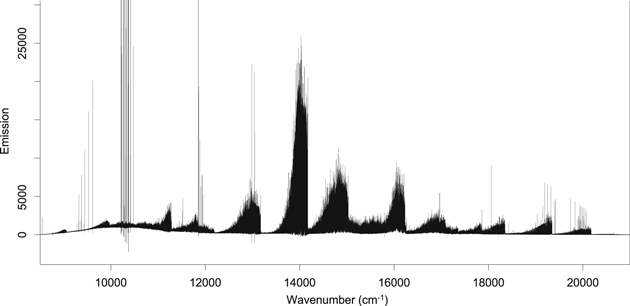
Figure 1. Raw overview emission spectrum of TiO with the y-axis in arbitrary units. Notice the strong Ti atomic lines and the thermal emission from the furnace in the baseline.
Download figure:
Standard image High-resolution imageOn the same day, three additional spectra were recorded. The first spectrum of the day was that of a standard tungsten filament lamp at 1.5 cm−1 resolution recorded through the furnace. The second spectrum was the TiO emission described above. The third spectrum was that of a quartz halogen lamp sent through the furnace, and the fourth spectrum bypassed the furnace and was just the lamp alone. These last two spectra had the same resolution as the TiO spectrum and their ratio gives a furnace transmission spectrum (τ), which can be converted to an absorbance (logarithm, base e) spectrum (Figure 2) for comparison with Figure 1.
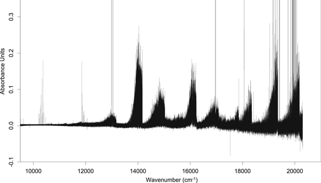
Figure 2. Overview absorption spectrum of TiO with the y-axis in absorbance units, i.e., −ln(τ). Notice the strong Ti atomic lines and the relatively poor signal-to-noise ratio.
Download figure:
Standard image High-resolution imageFigure 1 needs to be calibrated so the y-axis is an absorption cross section with the customary units of cm2/molecule and the x-axis is wavenumber corrected. These manipulations were carried out with the Bruker OPUS software. The first step was to Fourier interpolate the x-axis by a factor of 4 (by "zero-filling" the interferogram) to obtain more spectral points. The wavenumber calibration was carried out by multiplying the points on the x-axis by 1.000000303. This calibration factor was obtained using the lines of the  transition measured by Ram et al. (1999). The accuracy of the wavenumber calibration was assessed by comparison of the strong Ti atomic lines (Figure 1) with the Ritz wavenumber values in the NIST Atomic Spectra Database (Kramida et al. 2019). The wavenumber scale is accurate to about ±0.002 cm−1. The Ti atomic lines were then removed by replacing them with straight lines.
An attempt was made to correct the y-axis using the standard lamp spectrum and correcting for the frequency dependence of emission, but comparison with the absorption spectrum (Figure 2) showed that further correction was required. The baseline of this spectrum was first corrected by hand using OPUS. The absorbance spectrum was then used for a final intensity correction. From the Beer–Lambert law,  (Bernath 2020), the absorbance −ln(τ) is proportional to the absorption cross section σ, with x the column density. The intensities of 24 common lines from 13,172 to 20,178 cm−1 were measured in the two spectra and their ratios fitted with a third-order polynomial. The polynomial was used to create correction factors in Excel on a 1 cm−1 grid from 8500 to 21,000 cm−1. These correction factors were used in OPUS to provide absorption cross sections in arbitrary units. The intensity calibration to cm2/molecule units was carried out with ExoMol (McKemmish et al. 2019) and also depends on temperature.
The temperature of the furnace was measured, probably with an optical pyrometer, as 1950 K. To check this value, the 0-0 band of the  transition was simulated with PGOPHER (Western 2017) using the spectroscopic constants of Ram et al. (1999) and the temperature adjusted to match the observed spectrum. A value of 2300 K with an error of about 100 K was obtained. The 48Ti16O ExoMol lines (McKemmish et al. 2019) were converted to cross sections at 2300 K with a Doppler lineshape function using the ExoCross method (Yurchenko et al. 2018) conveniently available on the web at http://exomol.com/data/molecules/TiO/48Ti-16O/xsec-Toto/. The ExoMol cross sections were Fourier interpolated in OPUS by a factor of 2 to match the point spacing of 0.005 cm−1 of the observed cross sections. The A3Φ − X3Δ transition near 14,000 cm−1 (Figure 1) is strong and relatively unperturbed so was chosen for calibration. The observed A − X line widths are about 0.072 cm−1 compared to the Doppler line widths of 0.043 cm−1. The ExoMol cross sections were therefore convoluted using the Maple program with a Gaussian function of FWHM of 0.044 cm−1 (the instrumental resolution) and renormalized using the areas of three isolated A − X lines. Two other isolated 0-0 band lines at 14,122.154 cm−1 (Q3(36)) and 14,124.363 cm−1 (Q3(35)) were matched to better than 1% and provided the conversion from arbitrary units to cm2/molecule. The calibrated experimental cross sections (multiplied by 1018) are provided as data behind the figure and are plotted in Figure 3 along with the corresponding ExoMol cross sections.
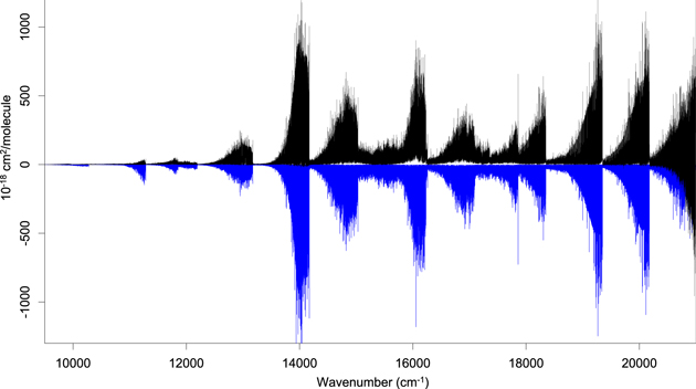
Figure 3. Experimental absorption cross sections of TiO at 2300 K and the corresponding ExoMol 48Ti16O cross sections, inverted for clarity.(The data used to create this figure are available.)
Download figure:
Standard image High-resolution image
3. Discussion and Conclusion
TiO cross sections can be used to derive column densities and concentrations in laboratory and astronomical sources. For example, using the same two lines of the 0-0 A − X band used for calibration yields a 48Ti16O column density of 1.95 × 10¹⁴ molecules cm−2 from the absorption spectrum (Figure 2) using the Beer–Lambert law. If the hearth in the carbon furnace is about 15 cm long (fairly typical for this source) then the concentration is about 1.3 × 10¹³ molecules cm−3.
The errors in the measured cross sections are difficult to assess since they are dominated by systematic errors. The experimental lifetimes (Hedgecock et al. 1995) for v = 0 of the three spin components of the A3Φ state differ by 8% from the values calculated by ExoMol (McKemmish et al. 2019). A conservative overall error estimate is thus about 10% for 13,178 to 20,178 cm−1 where absorption data (Figure 2) are available. The intensity calibration for 8500–13,178 cm−1 and higher than 20,178 cm−1 are extrapolated so are likely less reliable. However, the line intensities in the 0-0 band of the  transition near 9050 cm−1 are within 15% of the ExoMol values, although the line positions are off by more than 0.1 cm−1 (Bittner & Bernath 2018). For the 0-0 band of the
  transition near 11,272 cm−1, the line positions are accurate, but ExoMol intensities are too large by about a factor of 3 (Figure 3). The ExoMol 0-0 band
  intensities near 11,840 cm−1 agree reasonably well with the very blended observations, and the line positions match for low J, but begin to diverge for higher-J values. For the 0-0 band
  transition, many of the lines agree in position and intensity near 16,200 cm−1, but particularly to lower wavenumbers there seem to be many missing/shifted lines and intensity errors in ExoMol. Finally for the 0-0 band of the
  transition near 19,300 cm−1, the ExoMol line positions agree well with the observations, and the intensities are about 15% less than observed.
The observed TiO spectrum has many weak features that are assignable to the four minor isotopologues. The main purpose of this paper, however, is to provide experimental cross sections that can be used directly in the analysis of astronomical spectra. For the high-resolution cross-correlation method (Snellen et al. 2010) used to detect TiO in exoplanets (Nugroho et al. 2017), a high-quality template spectrum is needed. Using M-dwarf spectra, TiO templates based on ExoMol have been shown to be an improvement on previous line lists (McKemmish et al. 2019). However, the experimental cross sections can be used directly as long as the source temperature is reasonably close to 2300 K, as is often the case for hot Jupiter exoplanets and M stars.
The National Solar Observatory (NSO) is operated by the Association of Universities for Research in Astronomy, Inc. (AURA), under cooperative agreement with the National Science Foundation. The spectrum was recorded by S. Davis, G. Stark, J. Wagner, and R. Hubbard and was obtained from the NSO data archives. Financial support was provided by the NASA Exoplanet Program (grant NNX16AB51G).
Facility: McMath–Pierce Solar Telescope. -
Software: OPUS, Maple, PGOPHER (Western 2017), Excel.