


Abstract
PSR J1640+2224 is a binary millisecond pulsar (BMSP) with a white dwarf (WD) companion. Recent observations indicate that the WD is very likely to be a ∼0.7 M⊙ CO WD. Thus, the BMSP should have evolved from an intermediate-mass X-ray binary (IMXB). However, previous investigations on IMXB evolution predict that the orbital periods of the resultant BMSPs are generally < 40 days, in contrast with the 175 day orbital period of PSR J1640+2224. In this paper, we explore the influence of the mass of the neutron star (NS) and the chemical compositions of the companion star on the formation of BMSPs. Our results show that the final orbital period becomes longer with increasing NS mass, and the WD mass becomes larger with decreasing metallicity. In particular, to reproduce the properties of PSR J1640+2224, the NS was likely born massive (>2.0 M⊙).
Export citation and abstract BibTeX RIS
1. Introduction
Millisecond pulsars (MSPs) are neutron stars (NSs) with short spin periods (P ≤ 30 ms) and weak surface magnetic fields (B ∼ 108–109 G; Lorimer 2008). They are believed to be old NSs that have been reactivated by accretion from their companion stars during the low-mass X-ray binary (LMXB) phase (Alpar et al. 1982; Radhakrishnan & Srinivasan 1982). The mass transferred from the companion star not only causes the decay of the NS's magnetic field, but also accelerates the NS's spin period to milliseconds (see, e.g., Bhattacharya & van den Heuvel 1991; Tauris & van den Heuvel 2006, for reviews). This recycling scenario has been strongly supported by the discovery of several X-ray pulsars with millisecond periods in LMXBs (see Patruno & Watts 2012, for a summary), and the discovery of the transition between a rotation-powered MSP state and an LMXB state in PSR J1023+0038 (Archibald et al. 2009), IGR J18245-2452 (Papitto et al. 2013), and PSR J1227-4853 (Roy et al. 2015).
When the mass transfer ceases, some of the LMXBs evolve to be binary systems consisting of an MSP and a He white dwarf (WD). These populations are called low-mass binary pulsars (LMBPs) (Tauris & van den Heuvel 2006). Compared with LMBPs, there is another kind of population called intermediate-mass binary pulsars (IMBPs), which contain a pulsar with a spin period of tens of milliseconds and a CO or ONeMg WD with mass ≥0.4 M⊙ (Camilo et al. 1996, 2001; Chen et al. 2011). Most IMBPs are thought to have evolved from intermediate-mass X-ray binaries (IMXBs). Because of the relatively high mass ratio (q = M2/M1 > 1.5, where M1 and M2 are the NS mass and the donor star mass, respectively), it has been suggested that the mass transfer could be unstable, and the NS could spiral into the envelope of the donor in less than a millennium (Paczyński 1976; Webbink 1984; Iben & Livio 1993). More recent studies showed that X-ray binary systems with an intermediate-mass donor star may avoid entering the spiral-in phase, undergo rapid mass transfer on a (sub)thermal timescale, and eventually evolve into IMBPs (e.g., Kolb et al. 2000; Podsiadlowski & Rappaport 2000; Tauris et al. 2000; Shao & Li 2012). Since the birth rate of IMXBs is significantly larger than that of original LMXBs, and since IMXBs likely evolve to resemble observed LMXBs when the mass ratio becomes less than unity, it is generally believed that the majority of LMXBs may have started their lives with an intermediate-mass donor star (e.g., Pfahl et al. 2003).
PSR J1640+2224 is an MSP with a spin period P = 3.16 ms. It is located in a wide, nearly circular binary system (orbital period Porb = 175 days and orbital eccentricity e = 7.9725 × 10⁻⁴) with a WD companion (Lundgren et al. 1996). These characteristics seem to indicate that this system has evolved from a wide LMXB (Tauris 2011). According to the theoretical correlation between the orbital period and the WD mass (Rappaport et al. 1995; Tauris & Savonije 1999; Lin et al. 2011; Jia & Li 2014), the WD companion's mass would be ∼(0.35–0.39) M⊙ depending on the metallicity. Vigeland et al. (2018) recently presented the first astrometric parallax measurement of PSR J1640+2224, based on observations taken with the Very Long Baseline Array. Using the new distance in the analysis of the Hubble Space Telescope observation, they found that the WD mass is  and
and  for DA and DB WDs, respectively. The results indicate that the WD mass is larger than 0.4 M⊙ with >90%-confidence, so it is most likely a CO WD. However, previous works predicted that most IMBPs formed from IMXBs have a spin period of tens of milliseconds and an orbital period Porb < 40 days (Podsiadlowski & Rappaport 2000; Tauris et al. 2000; Podisadlowski et al. 2002; Pfahl et al. 2003; Shao & Li 2012). These characteristics are in conflict with the observational parameters of PSR J1640+2224. Therefore, the formation of this system had been a puzzle.
In this paper, we try to explore the formation route of PSR J1640+2224, paying particular attention to the influence of the NS mass and the metallicity of the donor star. The remainder of this paper is organized as follows. We describe the stellar evolution code and the binary model in Section 2. The calculated binary evolution results are demonstrated in Section 3. We present our discussion and summarize in Section 4.
2. Binary Evolutionary Calculations
2.1. The Stellar Evolution Code
All the calculations were carried out using the stellar evolution code Modules for Experiments in Stellar Astrophysics (version number 11554; Paxton et al. 2011, 2013, 2015, 2018, 2019). We have calculated the evolutions of a large number of I/LMXBs, adopting both Population I (X = 0.7 and Z = 0.02) and II (X = 0.75 and Z = 0.001) chemical compositions for the donor stars. For the treatment of convection in the donor stars, we employ both exponential diffusive overshooting with the parameter fov = 0.01–0.016 (Herwig 2000) and a mixing-length parameter of α = 2.0 (see Section 4). In our calculations, we have considered a number of binary interactions to follow the details of mass-transfer processes, including gravitational radiation (GR), magnetic braking (MB) and mass loss, which lead to orbital angular momentum loss.
2.2. The Input Physics
We assume that the binary initially consists of an NS of mass M1 and a zero-age main-sequence donor of mass M2. The Roche-lobe (RL) radius RL,2 of the donor is evaluated with the formula proposed by Eggleton (1983),

where a is the orbital separation of the binary and q = M2/M1 is the mass ratio. We adopt the Ritter (1988) scheme to calculate the mass-transfer rate via Roche-lobe overflow (RLOF),

where H is the scale height of the atmosphere evaluated at the surface of the donor, R2 is the radius of the donor, and

where ρ and  are the mass density and the sound speed on the surface of the star respectively, and Q is the cross section of the mass flow via the L1 point. The very small orbital eccentricity indicates that tides keep the binary orbit circular (King 1988), so the orbital angular momentum is

with the orbital angular velocity  (where M = M1 + M2 is the total mass). Taking the logarithmic derivative of Equation (4) with respect to time gives the rate of change in the orbital separation:

Here the total rate of change in the orbital angular momentum is determined by

The three terms on the right side of Equation (6) represent angular momentum losses caused by GR, MB, and mass loss, respectively. The GR-induced rate  is calculated with the standard formula (Landau & Lifshitz 1959; Faulkner 1971)

where G and c are the gravitational constant and the speed of light, respectively. The prescription of Verbuant & Zwaan (1981) is adopted to calculate the angular momentum loss due to MB,

For IMXBs and wide LMXBs, the mass-transfer rate  may be higher than the Eddington-limit accretion rate
  of the NS. Thus, the accretion rate of the NS is evaluated using

and the mass loss rate from the binary system is

In the case of super-Eddington accretion, we adopt the isotropic reemission model, assuming that the extra material leaves the binary in the form of isotropic wind from the NS. Therefore, the angular momentum loss rate due to mass loss can be derived to be

where a1 is the distance between the NS and the center of mass of the binary.
3. Results of Evolution Calculations
We have performed calculations of the binary evolution for thousands of I/LMXB systems. We choose the initial NS mass  and the initial donor mass
  , and set the initial orbital period 1.0 day
  days. We use exponential diffusive overshooting for the donor stars. Note that there exists a bifurcation period for the initial orbital period
  day (Pylyser & Savonije 1988, 1989). If the initial orbital period is below Pbf, the binary systems will evolve with shrinking orbits, possibly forming ultra-compact binaries. This kind of evolution cannot reproduce PSR J1640+2224, and will not be considered here. In addition, we exclude the evolutions with the final orbital periods exceeding 500 days.
3.1. A Typical Example for the IMXB Evolution
We present the evolutionary sequences for a typical IMXB system that consists of a 1.4 M⊙ NS and a 3.5 M⊙ donor star with an initial orbital period Porb = 6 days in Figures 1 and 2. The donor star starts to fill its RL and commence mass transfer at the age of 240.6 Myr. The mass-transfer process lasts about 1.9 Myr, at a rate higher than the Eddington accretion rate (the maximum mass-transfer rate >10−5 M⊙ yr−1). In this case, most of the transferred material from the donor is lost from the binary system. Thus, after the mass transfer, the donor evolves into a CO WD of mass 0.543 M⊙, while the NS has accreted only 0.034 M⊙ mass. The orbital period becomes smaller in the former stage of the mass-transfer process due to the relatively high mass ratio (>1); when the mass ratio is reversed, the orbit begins to expand. The final orbital period is Porb = 17.8 days.
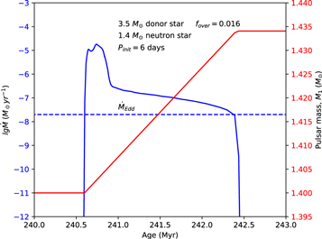
Figure 1. Example evolution of a typical IMXB consisting of a NS and a donor star with initial masses M1 = 1.4 M⊙ and M2 = 3.5 M⊙ respectively, and orbital period Porb = 6 days. The blue and red solid curves denote the evolutionary tracks for the mass-transfer rate and the NS mass, respectively, and the blue dashed curve denotes the Eddington-limit accretion rate.
Download figure:
Standard image High-resolution image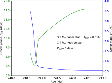
Figure 2. Same as Figure 1. The green and blue curves denote the evolutionary tracks for the orbital period and the donor mass, respectively.
Download figure:
Standard image High-resolution image3.2. The  Diagram

Figure 3 shows the calculated final orbital period as a function of the WD mass for different initial masses of the donor star and the NS. The yellow, green, red, and blue curves are for NSs with initial masses 1.4 M⊙, 1.8 M⊙, 2.0 M⊙, and 2.2 M⊙, respectively. Beside each curve we label the initial mass of the donor star. The triangles are used to denote the final systems with the longest orbital periods for a given donor star, and also to distinguish different curves that overlap. The gray horizontal line represents the orbital period–WD mass distribution for PSR J1640+2224.

Figure 3. Final orbital period as a function of WD mass. The yellow, green, red and blue curves are for initial NS masses of 1.4 M⊙, 1.8 M⊙, 2.0 M⊙, and 2.2 M⊙, respectively. Beside each curve we label the initial donor mass. The gray, solid horizontal line represents the distribution of the orbital period and the WD mass for PSR J1640+2224. The triangles are used to distinguish different curves that overlap. In the top and bottom panels we adopt different chemical compositions and overshooting parameters (top: Population I and fov = 0.016; bottom: Population II and fov = 0.01).
Download figure:
Standard image High-resolution imageIn the top panel we show the results with Population I chemical compositions. We first examine the orbital period–WD mass relation for a 1.4 M⊙ NS. In this case, it is clear to that, for a given WD mass > 0.4 M⊙, the predicted final orbital period is significantly shorter than 175 days. For a more massive donor star, the resultant WD is more massive, while the final orbital period is shorter. So they are obviously unable to account for the properties of PSR J1640+2224. If we increase the mass of the NS, the final orbital period becomes longer. When M1 = 2.0 M⊙, it is possible to simultaneously account for the WD of mass ∼0.4 M⊙ and the orbital period ∼ 175 days. Moreover, if the WD is more massive than 0.6 M⊙, then the initial NS mass should be enhanced to be 2.2 M⊙.
The bottom panel shows the results with Population II chemical compositions. It is known that lower metallicities lead to smaller stellar radius and shorter nuclear evolutionary timescale. So stars with the same mass but lower metallicities form WDs in a narrower orbit (Tauris & Savonije 1999; Jia & Li 2014). We can see that the evolution of LMXBs containing a 1.4 M⊙ NS and a 1.0 M⊙ donor star may form PSR J1640+2224-like binaries with a 0.4 M⊙ WD companion. However, if the WD indeed has a mass higher than 0.6 M⊙, then we still require the NS to be initially more massive than 2.0 M⊙.
We summarize our calculated results with MWD ≥ 0.4 M⊙ and the final orbital period  days in Table 1. Note that PSR J1640+2224 most likely descended from an IMXB via Case B RLOF. Tables 2–5 present more general results by taking into account different initial NS mass.
Table 1. Parameters for IMXB Evolution with the Final Orbit Period 170 days ≤ Porb ≤ 180 days and the WD Mass MWD ≥ 0.4 M⊙

|

|

|

|

|

|

|
Type |

|

|

|
|---|---|---|---|---|---|---|---|---|---|---|
| (M⊙) | (M⊙) | (days) | (Myr) | (M⊙) | (M⊙) | (days) | (M⊙) | (Myr) | (M⊙ yr−1) | |
| (1) | (2) | (3) | (4) | (5) | (6) | (7) | (8) | (9) | (10) | (11) |
| Population I (X = 0.7, Z = 0.02) | ||||||||||
| 2.0 | 2.5 | 5.35 | 597.900 | 2.109 | 0.414 | 170.0 | HeCO | 0.109 | 5.845 | 3.16 × 10⁻⁴ |
| 2.2 | 2.5 | 7.0 | 598.596 | 2.304 | 0.488 | 175.0 | CO | 0.104 | 6.580 | 5.01 × 10⁻⁶ |
| 2.2 | 3.0 | 7.0 | 363.239 | 2.255 | 0.506 | 176.5 | CO | 0.055 | 3.363 | 7.94 × 10⁻⁶ |
| 2.2 | 3.5 | 10.8 | 241.819 | 2.226 | 0.571 | 171.5 | CO | 0.026 | 1.558 | 2.51 × 10⁻⁵ |
| 2.25 | 4.0 | 15.2 | 170.965 | 2.266 | 0.634 | 170.8 | CO | 0.016 | 0.857 | 6.31 × 10⁻⁵ |
| Population II (X = 0.75, Z = 0.001) | ||||||||||
| 1.4 | 1.0 | 29.0 | 5965.290 | 1.732 | 0.400 | 177.9 | He | 0.332 | 19.440 | 7.00 × 10⁻⁸ |
| 1.4 | 1.5 | 17.0 | 1557.870 | 1.837 | 0.400 | 173.9 | He | 0.437 | 27.950 | 3.16 × 10⁻⁷ |
| 1.8 | 1.5 | 12.5 | 1547.698 | 2.427 | 0.400 | 175.4 | He | 0.627 | 38.912 | 7.59 × 10⁻⁸ |
| 1.8 | 2.0 | 12.0 | 642.987 | 2.046 | 0.479 | 171.4 | CO | 0.246 | 13.620 | 1.58 × 10⁻⁶ |
| 2.0 | 1.5 | 11.5 | 1544.370 | 2.694 | 0.400 | 178.3 | He | 0.694 | 42.240 | 5.89 × 10⁻⁸ |
| 2.0 | 2.0 | 10.5 | 650.153 | 2.293 | 0.484 | 174.1 | CO | 0.293 | 16.379 | 5.01 × 10⁻⁷ |
| 2.0 | 2.5 | 10.5 | 370.271 | 2.110 | 0.525 | 174.3 | CO | 0.110 | 6.503 | 7.94 × 10⁻⁶ |
| 2.2 | 1.5 | 10.5 | 1540.127 | 2.965 | 0.400 | 176.9 | He | 0.756 | 46.617 | 4.37 × 10⁻⁸ |
| 2.2 | 2.0 | 9.0 | 648.640 | 2.524 | 0.484 | 170.7 | CO | 0.324 | 13.085 | 3.16 × 10⁻⁷ |
| 2.2 | 2.5 | 8.5 | 369.724 | 2.32 | 0.525 | 173.2 | CO | 0.120 | 7.045 | 6.31 × 10⁻⁶ |
| 2.2 | 3.0 | 12.3 | 236.243 | 2.262 | 0.616 | 178.8 | CO | 0.062 | 4.155 | 2.85 × 10⁻⁵ |
| 2.2 | 3.5 | 19.0 | 169.025 | 2.246 | 0.723 | 177.3 | CO | 0.046 | 3.098 | 7.94 × 10⁻⁵ |
| 2.2 | 4.0 | 25.5 | 125.904 | 2.231 | 0.794 | 170.0 | CO | 0.031 | 1.760 | 2.00 × 10⁻⁴ |
Note. Column (1): the initial NS mass. Column (2): the initial donor mass. Column (3): the initial orbital period. Column (4): the age of the donor star at the onset of RLOF. Column (5): the final mass of the NS. Column (6): the final mass of the WD. Column (7): final orbital period. Column (8): the type of the WD. Column (9): the mass accreted by the NS. Column (10): the duration of the mass transfer. Column (11): the maximum mass-transfer rate.
Download table as: ASCIITypeset image
Table 2.
Calculated Results of the Binary Evolution with 
| Population I; fov = 0.016 | Population II; fov = 0.01 | ||||||||||
|---|---|---|---|---|---|---|---|---|---|---|---|
| M2,i |

|
Case |

|

|

|

|

|
Case |

|

|

|
| (M⊙) | (days) | (RLO) | (M⊙) | (M⊙) | (days) | (M⊙) | (days) | (RLO) | (M⊙) | (M⊙) | (days) |
| 1.0 | 3.0 | B | 2.069 | 0.264 | 19.7 | 1.0 | 3.0 | B | 2.037 | 0.300 | 25.8 |
| 5.0 | B | 2.040 | 0.294 | 52.9 | 5.0 | B | 2.015 | 0.324 | 43.4 | ||
| 10.0 | B | 1.994 | 0.316 | 97.5 | 10.0 | B | 1.966 | 0.350 | 75.9 | ||
| 20.0 | B | 1.890 | 0.338 | 172.0 | 20.0 | B | 1.866 | 0.379 | 129.4 | ||
| 60.0 | B | 16.22 | 0.382 | 436.1 | 60.0 | B | 1.576 | 0.437 | 317.0 | ||
| 1.5 | 3.0 | B | 2.389 | 0.281 | 34.9 | 1.5 | 2.0 | B | 2.158 | 0.304 | 27.1 |
| 4.0 | B | 2.282 | 0.301 | 62.9 | 6.0 | B | 2.165 | 0.351 | 76.1 | ||
| 6.0 | B | 2.179 | 0.316 | 95.7 | 10.0 | B | 2.025 | 0.373 | 113.0 | ||
| 10.0 | B | 2.089 | 0.333 | 147.1 | 20.0 | B | 1.784 | 0.407 | 199.1 | ||
| 20.0 | B | 1.827 | 0.358 | 267.1 | 60.0 | B | 1.539 | 0.471 | 464.5 | ||
| 2.0 | 1.5 | A | 2.707 | 0.290 | 38.0 | 2.0 | 1.0 | A | 1.635 | 0.324 | 21.3 |
| 2.0 | B | 2.058 | 0.305 | 51.1 | 2.0 | B | 1.604 | 0.337 | 39.1 | ||
| 2.5 | B | 1.886 | 0.317 | 58.8 | 3.0 | B | 1.619 | 0.346 | 54.1 | ||
| 2.5 | 1.5 | A | 2.469 | 0.275 | 18.0 | 5.0 | B | 1.649 | 0.374 | 74.6 | |
| 2.0 | B | 1.624 | 0.345 | 32.7 | 2.5 | 1.0 | A | 1.526 | 0.395 | 11.8 | |
| 3.0 | B | 1.555 | 0.365 | 44.5 | 2.0 | B | 1.465 | 0.424 | 20.6 | ||
| 4.0 | B | 1.526 | 0.373 | 57.3 | 4.0 | B | 1.448 | 0.436 | 38.9 | ||
| 3.0 | 1.5 | A | 2.171 | 0.270 | 16.4 | 6.0 | B | 1.446 | 0.447 | 55.1 | |
| 2.0 | A | 1.964 | 0.373 | 15.5 | 8.0 | B | 1.445 | 0.468 | 66.7 | ||
| 4.0 | B | 1.466 | 0.440 | 27.1 | 3.0 | 1.0 | A | 1.481 | 0.462 | 6.1 | |
| 6.0 | B | 1.456 | 0.447 | 39.6 | 3.0 | B | 1.428 | 0.534 | 13.5 | ||
| 3.5 | 1.5 | A | 2.015 | 0.253 | 11.1 | 5.0 | B | 1.421 | 0.540 | 26.4 | |
| 2.0 | A | 1.786 | 0.379 | 9.8 | 8.0 | B | 1.419 | 0.541 | 35.0 | ||
| 3.0 | B | 1.444 | 0.511 | 9.2 | 12.0 | B | 1.417 | 0.547 | 51.3 | ||
| 5.0 | B | 1.434 | 0.527 | 14.4 | 3.5 | 1.0 | A | 1.450 | 0.531 | 3.0 | |
| 8.0 | B | 1.428 | 0.535 | 22.4 | 2.0 | B | 1.419 | 0.644 | 3.9 | ||
| 4.0 | 3.0 | B | 1.430 | 0.572 | 4.3 | 3.0 | B | 1.415 | 0.650 | 5.7 | |
| 4.0 | B | 1.422 | 0.600 | 5.2 | 5.0 | B | 1.413 | 0.660 | 9.3 | ||
| 5.0 | B | 1.421 | 0.605 | 6.3 | 8.0 | B | 1.412 | 0.661 | 14.9 | ||
| 6.0 | B | 1.419 | 0.616 | 7.3 | 12.0 | B | 1.413 | 0.663 | 22.1 | ||
Download table as: ASCIITypeset image
Table 3.
Calculated Results of the Binary Evolution with 
Population I; 
|
Population II; 
|
||||||||||
|---|---|---|---|---|---|---|---|---|---|---|---|

|

|
Case |

|

|

|

|

|
Case |

|

|

|
| (M⊙) | (days) | (RLO) | (M⊙) | (M⊙) | (days) | (M⊙) | (days) | (RLO) | (M⊙) | (M⊙) | (days) |
| 1.5 | 3.0 | B | 2.877 | 0.295 | 53.4 | 1.5 | 1.5 | A | 2.700 | 0.276 | 16.2 |
| 4.0 | B | 2.816 | 0.312 | 85.1 | 3.0 | B | 2.827 | 0.336 | 56.9 | ||
| 8.0 | B | 2.659 | 0.337 | 161.7 | 10.0 | B | 2.536 | 0.387 | 145.8 | ||
| 15.0 | B | 2.408 | 0.363 | 277.1 | 20.0 | B | 2.228 | 0.425 | 258.7 | ||
| 2.0 | 2.0 | A | 2.468 | 0.322 | 75.1 | 40.0 | B | 2.025 | 0.466 | 434 | |
| 3.0 | B | 2.229 | 0.335 | 101.2 | 2.0 | 1.0 | A | 2.131 | 0.363 | 36.3 | |
| 6.0 | B | 2.227 | 0.353 | 172.8 | 3.0 | B | 2.080 | 0.378 | 77 | ||
| 9.0 | B | 2.204 | 0.368 | 234.0 | 10.0 | B | 2.066 | 0.475 | 143.2 | ||
| 15.0 | B | 2.142 | 0.387 | 350.4 | 20.0 | B | 1.937 | 0.492 | 283.1 | ||
| 2.5 | 1.5 | A | 3.067 | 0.299 | 62.9 | 60.0 | B | 1.833 | 0.549 | 663.9 | |
| 2.0 | A | 2.439 | 0.350 | 74.0 | 2.5 | 1.0 | A | 1.944 | 0.397 | 26 | |
| 3.0 | B | 1.976 | 0.377 | 93.8 | 3.0 | B | 1.862 | 0.446 | 59.8 | ||
| 4.0 | B | 1.947 | 0.387 | 118.3 | 5.0 | B | 1.852 | 0.502 | 74.9 | ||
| 3.0 | 1.5 | A | 2.878 | 0.299 | 43.0 | 10.0 | B | 1.885 | 0.530 | 126.0 | |
| 2.0 | A | 2.628 | 0.378 | 42.0 | 3.0 | 1.0 | A | 1.890 | 0.468 | 16.1 | |
| 3.0 | B | 1.879 | 0.440 | 54.9 | 3.0 | B | 1.830 | 0.537 | 35 | ||
| 4.0 | B | 1.870 | 0.445 | 71.3 | 5.0 | B | 1.823 | 0.547 | 56.1 | ||
| 6.0 | B | 1.862 | 0.455 | 101.4 | 10.0 | B | 1.837 | 0.598 | 107.4 | ||
| 3.5 | 1.5 | A | 2.667 | 0.301 | 39.1 | 3.5 | 1.0 | A | 1.985 | 0.524 | 9.4 |
| 2.0 | A | 2.359 | 0.394 | 32.6 | 3.0 | B | 1.824 | 0.660 | 17.7 | ||
| 4.0 | B | 1.839 | 0.526 | 37.7 | 5.0 | B | 1.817 | 0.666 | 28.8 | ||
| 6.0 | B | 1.832 | 0.537 | 53.9 | 10.0 | B | 1.817 | 0.670 | 56.1 | ||
| 9.0 | B | 1.828 | 0.543 | 78.8 | 15.0 | B | 1.816 | 0.672 | 32.6 | ||
| 4.0 | 1.5 | A | 2.552 | 0.298 | 30.2 | 4.0 | 1.0 | A | 2.013 | 0.556 | 6 |
| 2.0 | A | 2.165 | 0.405 | 25.0 | 3.0 | B | 1.816 | 0.746 | 10.2 | ||
| 3.0 | B | 1.826 | 0.605 | 15.0 | 5.0 | B | 1.813 | 0.762 | 16.2 | ||
| 6.0 | B | 1.819 | 0.623 | 28.0 | 12.0 | B | 1.811 | 0.776 | 38.0 | ||
| 10.0 | B | 1.815 | 0.643 | 43.4 | 20.0 | B | 1.810 | 0.779 | 62.8 | ||
Download table as: ASCIITypeset image
Table 4.
Calculated Results of the Binary Evolution with 
| Population I; fov = 0.016 | Population II; fov = 0.01 | ||||||||||
|---|---|---|---|---|---|---|---|---|---|---|---|
| M2,i |

|
Case |

|

|

|

|

|
Case |

|

|

|
| (M⊙) | (days) | (RLO) | (M⊙) | (M⊙) | (days) | (M⊙) | (days) | (RLO) | (M⊙) | (M⊙) | (days) |
| 1.5 | 3.0 | B | 3.082 | 0.300 | 61.3 | 1.5 | 2.0 | B | 2.861 | 0.322 | 42.2 |
| 4.0 | B | 3.049 | 0.315 | 94.3 | 5.0 | B | 2.977 | 0.361 | 92.8 | ||
| 6.0 | B | 2.975 | 0.330 | 139.2 | 10.0 | B | 2.769 | 0.393 | 158.7 | ||
| 10.0 | B | 2.863 | 0.348 | 212.6 | 20.0 | B | 2.44 | 0.431 | 281.4 | ||
| 20.0 | B | 2.493 | 0.378 | 391.6 | 40.0 | B | 2.233 | 0.473 | 475 | ||
| 2.0 | 2.0 | A | 2.681 | 0.325 | 87.5 | 2.0 | 1.0 | A | 2.365 | 0.331 | 43.0 |
| 3.0 | B | 2.464 | 0.340 | 117.9 | 3.0 | B | 2.337 | 0.390 | 81.4 | ||
| 6.0 | B | 2.459 | 0.360 | 199.1 | 6.0 | B | 2.318 | 0.477 | 99.8 | ||
| 9.0 | B | 2.429 | 0.374 | 272.2 | 10.0 | B | 2.283 | 0.487 | 162.9 | ||
| 15.0 | B | 2.355 | 0.395 | 406.8 | 15.0 | B | 2.205 | 0.512 | 225.4 | ||
| 2.5 | 1.5 | A | 3.326 | 0.309 | 78.9 | 2.5 | 1.0 | A | 2.149 | 0.397 | 33.8 |
| 2.0 | A | 2.705 | 0.350 | 94.1 | 3.0 | B | 2.068 | 0.469 | 69.0 | ||
| 3.0 | B | 2.183 | 0.380 | 119.8 | 8.0 | B | 2.105 | 0.528 | 131.2 | ||
| 5.0 | B | 2.114 | 0.407 | 166.2 | 16.0 | B | 2.095 | 0.538 | 253.1 | ||
| 3.0 | 1.5 | A | 3.138 | 0.309 | 64.9 | 3.0 | 1.0 | A | 2.094 | 0.467 | 22.5 |
| 2.0 | A | 2.847 | 0.382 | 61.1 | 3.0 | B | 2.030 | 0.527 | 51.1 | ||
| 3.0 | B | 2.091 | 0.437 | 78.4 | 8.0 | B | 2.050 | 0.597 | 98.6 | ||
| 7.0 | B | 2.055 | 0.479 | 148.7 | 15.0 | B | 2.056 | 0.624 | 163.3 | ||
| 3.5 | 1.5 | A | 2.928 | 0.315 | 56.9 | 3.5 | 1.0 | A | 2.200 | 0.525 | 14.2 |
| 2.0 | A | 2.634 | 0.397 | 48.7 | 2.0 | B | 2.024 | 0.614 | 20.7 | ||
| 3.0 | B | 2.051 | 0.509 | 45.9 | 6.0 | B | 2.013 | 0.644 | 55.6 | ||
| 6.0 | B | 2.032 | 0.540 | 79.2 | 10.0 | B | 2.013 | 0.652 | 89.9 | ||
| 10.0 | B | 2.027 | 0.549 | 127.1 | 18.0 | B | 2.032 | 0.711 | 130.4 | ||
| 4.0 | 1.5 | A | 2.761 | 0.316 | 49.1 | 4.0 | 1.0 | A | 2.231 | 0.562 | 9.6 |
| 2.0 | A | 2.404 | 0.408 | 40.6 | 2.0 | B | 2.022 | 0.705 | 12.2 | ||
| 3.0 | B | 2.030 | 0.591 | 25.6 | 6.0 | B | 2.014 | 0.740 | 32.9 | ||
| 6.0 | B | 2.020 | 0.626 | 44.1 | 12.0 | B | 2.012 | 0.750 | 64.0 | ||
| 12.0 | B | 2.017 | 0.625 | 88.9 | 20.0 | B | 2.011 | 0.756 | 104.5 | ||
Download table as: ASCIITypeset image
Table 5.
Calculated Results of the Binary Evolution with 
| Population I; fov = 0.016 | Population II; fov = 0.01 | ||||||||||
|---|---|---|---|---|---|---|---|---|---|---|---|
| M2,i |

|
Case |

|

|

|

|

|
Case |

|

|

|
| (M⊙) | (days) | (RLO) | (M⊙) | (M⊙) | (days) | (M⊙) | (days) | (RLO) | (M⊙) | (M⊙) | (days) |
| 1.5 | 3.0 | B | 3.285 | 0.304 | 68.5 | 1.5 | 1.5 | A | 3.079 | 0.298 | 24.5 |
| 5.0 | B | 3.239 | 0.327 | 127.9 | 5.0 | B | 3.203 | 0.365 | 99.5 | ||
| 10.0 | B | 3.093 | 0.352 | 228.8 | 10.0 | B | 2.993 | 0.397 | 170.1 | ||
| 20.0 | B | 2.704 | 0.382 | 422.1 | 20.0 | B | 2.650 | 0.436 | 300.8 | ||
| 40.0 | B | 2.483 | 0.415 | 729.1 | 40.0 | B | 2.439 | 0.479 | 504.2 | ||
| 2.0 | 1.5 | A | 3.563 | 0.314 | 73.1 | 2.0 | 1.0 | A | 2.592 | 0.334 | 49.1 |
| 4.0 | B | 2.694 | 0.351 | 166.4 | 5.0 | B | 2.525 | 0.472 | 99.4 | ||
| 8.0 | B | 2.658 | 0.376 | 280.3 | 10.0 | B | 2.477 | 0.480 | 198.4 | ||
| 12.0 | B | 2.599 | 0.392 | 384.5 | 20.0 | B | 2.365 | 0.506 | 364.1 | ||
| 15.0 | B | 2.565 | 0.401 | 456.8 | 60.0 | B | 2.243 | 0.554 | 894.0 | ||
| 2.5 | 1.5 | A | 3.572 | 0.320 | 89.3 | 2.5 | 1.0 | A | 2.362 | 0.400 | 41.1 |
| 4.0 | B | 2.344 | 0.409 | 163.9 | 3.0 | B | 2.264 | 0.489 | 76.5 | ||
| 8.0 | B | 2.313 | 0.490 | 196.5 | 8.0 | B | 2.300 | 0.533 | 157.5 | ||
| 12.0 | B | 2.312 | 0.494 | 288.1 | 20.0 | B | 2.095 | 0.552 | 364.6 | ||
| 17.0 | B | 2.303 | 0.500 | 396.1 | 40.0 | B | 2.095 | 0.661 | 463 | ||
| 3.0 | 1.5 | A | 3.339 | 0.321 | 91.7 | 3.0 | 1.0 | A | 2.295 | 0.469 | 29.1 |
| 2.0 | A | 2.998 | 0.386 | 82.9 | 3.0 | B | 2.231 | 0.542 | 61.8 | ||
| 4.0 | B | 2.276 | 0.457 | 121.5 | 8.0 | B | 2.251 | 0.608 | 121.2 | ||
| 8.0 | B | 2.244 | 0.516 | 187.8 | 15.0 | B | 2.249 | 0.633 | 204.6 | ||
| 3.5 | 1.5 | A | 3.168 | 0.325 | 76.5 | 3.5 | 1.0 | A | 2.471 | 0.520 | 19.5 |
| 3.0 | A | 2.252 | 0.511 | 62.7 | 2.0 | B | 2.223 | 0.653 | 24.2 | ||
| 5.0 | B | 2.235 | 0.538 | 91.5 | 6.0 | B | 2.218 | 0.667 | 69.5 | ||
| 8.0 | B | 2.230 | 0.551 | 138.2 | 10.0 | B | 2.218 | 0.696 | 105.7 | ||
| 11.5 | B | 2.225 | 0.582 | 168.2 | 20.0 | B | 2.240 | 0.752 | 169.4 | ||
| 4.0 | 1.5 | A | 2.998 | 0.330 | 69.3 | 4.0 | 1.0 | A | 2.452 | 0.562 | 14.1 |
| 3.0 | A | 2.225 | 0.617 | 33.3 | 2.0 | A | 2.222 | 0.731 | 16.2 | ||
| 6.0 | B | 2.220 | 0.628 | 63.5 | 6.0 | B | 2.212 | 0.775 | 43.3 | ||
| 9.0 | B | 2.216 | 0.643 | 89.8 | 10.0 | B | 2.212 | 0.778 | 71.4 | ||
| 15.0 | B | 2.216 | 0.632 | 156.8 | 20.0 | B | 2.240 | 0.787 | 138.5 | ||
Download table as: ASCIITypeset image
3.3. Further Constraints from Spin Evolution
Next we examine whether the mass transfer can accelerate the NS's spin period to milliseconds. The spin-up rate of the NS in an LMXB is determined by the rate of angular momentum transfer due to mass accretion,

where P and  are the spin period and its derivative of the NS, respectively, and R1 is the radius of the NS. Here we have assumed that the NS's magnetic field has been decayed so much that the accretion disk can extend to the surface of the NS. The amount of accreted mass needed to produce a MSP can be roughly estimated to be
The actual value of  could be smaller by a factor of ∼2 than that in Equation (13) if considering the effect of the NS magnetic field–accretion disk interaction. Combing this with Table 1, we note that evolutions with Population II compositions seem to be more preferred for the formation of PSR J1640+2224.
Figure 4 shows an example of the Population II evolutionary paths for PSR J1640+2224, which are able to reproduce the observed parameters of PSR J1640+2224. The evolution of this X-ray binary starts with a 2.2 M⊙ NS and a 3.0 M⊙ donor star in a 12.3 day orbit. The left panels show the evolution of Porb, M1, and  as a function of the donor mass, and the right panels show the evolution of
  and the chemical composition of the donor star. At the age of t = 236 Myr the donor star overflows its RL and transfers mass to the NS at a rate well above the Eddington-limit accretion rate. Accordingly, the mass transfer lasts ∼1.1 Myr, and the donor loses ∼3.1 M⊙ mass. Due to the extensive mass loss, the orbital period does not decrease significantly. Then the donor star shrinks and becomes detached from its RL. The next mass-transfer phase lasts ∼3.0 Myr, with a rate
  yr−1. After the mass transfer, the NS has accreted material of
  . The endpoint of the evolution is a binary consisting of a recycled pulsar and a CO WD with a mass of 0.616 M⊙.

Figure 4. Evolution of an IMXB with the initial NS mass, donor mass, and orbital period M1 = 2.2 M⊙, M2 = 3.0 M⊙, and Porb = 12.3 days, respectively. The left panels show the evolution of Porb, M1, and  as a function of the donor mass, and the right panels show the evolution of
  and chemical composition for the donor star as a function of time.
Download figure:
Standard image High-resolution image4. Discussion and Conclusions
The observed properties of PSR J1640+2224, such as its short spin period (3.16 ms), high WD mass (M2 ≥ 0.4 M⊙ with > 90% confidence), long orbital period (175 days), and nearly circular orbit (e = 7.9725 × 10⁻⁴), make it distinct from other MSPs and imply something unusual in its evolutionary history.
In this work, we have attempted to explore which evolutionary channels can reproduce the observed parameters of PSR J1640+2224. To achieve this goal, we consider different NS mass, donor mass, and metal abundance (Z = 0.02 and 0.001). Our main results are presented in Figure 3 and Tables 1–5, and can be summarized as follows.
- 1.For Population I chemical compositions, when, it is possible to simultaneously account for the WD mass (∼0.4 M⊙) and the orbital period (∼175 days). But if the WD mass , the NS mass should be larger than 2.2 M⊙, and the donor star must initially be intermediate-mass.
- 2.For Population II chemical compositions, the evolution of original LMXBs containing a 1.4 M⊙ NS and a 1.0 M⊙ donor star may form PSR J1640+2224-like binaries with a 0.4 M⊙ WD companion. However, if the WD indeed has a mass higher than 0.6 M⊙, then the initial NS mass should be no less than 2.0 M⊙, and the initial donor mass should be higher than 3.0 M⊙.
- 3.When the NS spin evolution is taken into account, the evolutions with Population II compositions seem to be more preferred for the formation of PSR J1640+2224.


Almost all of our results predict an NS of initial mass higher than 2.0 M⊙ (see Table 1). It is noted that Fonseca et al. (2016) demonstrated that J1640+2224 is likely a massive NS ( ) by analyzing the North American Nanohertz Observatory for Gravitational Waves (NANOGrav) 9 yr data set, although there are large uncertainties on the pulsar mass.
The birth masses of NSs depend on the physical mechanisms in core-collapse supernova explosions of massive stars, which are still highly uncertain (Timmes et al. 1996; Janka 2012). Theoretical studies do claim that NSs could be born massive. For example, by simulating neutrino-powered supernova explosions in spherical symmetry, Ugliano et al. (2012) found that the birth masses of NSs vary within a range of 1.2–2.0 M⊙. Pejcha & Thompson (2015) also numerically investigated the possible scope of the birth masses of NSs, and found that they could be as high as 1.9 M⊙. Sukhbold et al. (2016) presented supernova simulations for a grid of massive stars and obtained the birth masses of NSs ranging from 1.2 M⊙ to 1.8 M⊙.
Observationally, supermassive NSs have been discovered in quite a few X-ray binaries and binary MSPs (Antoniadis et al. 2016). However, since they have experienced mass-transfer processes, their current masses may not properly reflect their birth masses. For NSs in high-mass X-ray binaries (HMXBs), because they are relatively young (with an age ≲107 yr) and the efficiency of wind accretion is very low, their masses should be very close to those at birth (Shao & Li 2012). In HMXBs, the maximum NS mass measured is 2.12 ± 0.16 M⊙ for Vela X-1 (Rawls et al. 2011; Falanga et al. 2015). For binary MSPs, the masses of supermassive NSs span between ∼2.0 M☉ and ∼2.9 M⊙ (Linares 2019, for a recent review). For example, PSR J0740+6620 is one of the most massive NSs ever accurately measured, with a mass  (Cromartie et al. 2020), a spin period of 2.88 ms and a He WD companion of mass
  . These parameters mean that PSR J0740+6620 should have experienced extensive mass accretion during the LMXB phase, so its current mass may not represent its birth mass. However, recent studies suggested that mass transfer in LMXBs is likely to be highly non-conservative even at sub-Eddington mass-transfer rates (e.g., Lin et al. 2011; Tauris et al. 2011; Antoniadis et al. 2013; Fortin et al. 2016). Our results show that, even with Eddington-limited accretion, a supermassive newborn NS is still required, at least for PSR J1640+2224.
We need to mention that our results are subject to several uncertainties, such as the treatment of convection in the donor star and the accretion efficiency during the mass-transfer process. The convective overshooting parameter plays an important role in our work. Up to the present time two standard methods have been used in modeling overshooting in numerical calculation. The first one is based on a simple extension of the the convectively mixed region above the boundary defined by the Schwarzschild criterion. This extension lov is parameterized in terms of the local pressure scale height HP at the boundary,

where α is the convective overshooting parameter. In this model, various attempts have been undertaken to constrain the value of α. Schröder et al. (1997) derived it to be 0.25 and 0.32 for stars in the mass range of (2.5–7) M⊙ for eclipsing binary stars. Ribas et al. (2000) and Claret (2007) found that the value of α is in the range of 0.1–0.6, and the amount of overshooting increases systematically with the stellar mass. Shibahashi et al. (2012) used asteroseismic analysis and obtained α = 0.1–0.3 for β Cephei stars (with mass M ≥ 8 M⊙). Degroote et al. (2010) analyzed the period space of SPB star HD 50230 (M = 7–8 M⊙) and suggested that the overshooting extent of the convective core is about (0.2–0.3) HP. Pápics et al. (2014) analyzed the period spacings of KIC 10526294 (M = 3.25 M⊙) and suggested that α is less than or equal to 0.15.
In an alternative approach, convective overshooting is considered to be a diffusive process with a diffusion parameter
where z is the radial distance from the formal Schwarzschild border and fov is a free parameter, and D0 is set as the scale of diffusive speed and derived from the convective velocity obtained from the mixing-length theory and taken below the Schwarzschild boundary (Herwig 2000).
Herwig (2000) investigated the evolution of AGB stars with convective overshooting and set the diffusive convective parameter fov = 0.016, which is widely adopted. Moravveji et al. (2015) analyzed KIC 10526294 with both the step function overshooting and exponentially decreasing overshooting, and found that the latter is better than the former for interpreting the observations with fov = 0.017–0.018. Moravveji et al. (2016) obtained fov = 0.024 ± 0.001 for KIC 7760680. Based on the k − ω model, Guo & Li (2019) concluded that fov is about 0.008 for stars in the mass range of (1.0–1.8) M⊙.
In Table 6, we compare the calculated results for I/LMXB evolution with different overshooting parameters (α = 0.2, 0.335 and fov = 0.016). The initial NS and donor masses are taken to be M1 = 2.0 M⊙ and M2 = 2.5 M⊙, respectively. From the results in Table 6, we conclude that the overshooting model with α = 0.2 is nearly the same as the diffusive overshooting model with fov = 0.016, and that increasing the value of α to 0.335 would result in more massive WDs and shorter orbital periods with the same initial parameters.
Table 6. IMXB Evolution with Different Overshoot Parameters
 , M2 = 2.5 M⊙ , M2 = 2.5 M⊙ |
||||||
|---|---|---|---|---|---|---|

|
α = 0.2 | α = 0.335 | ||||

|

|

|

|

|

|

|
| (day) | (M⊙) | (day) | (M⊙) | (day) | (M⊙) | (day) |
| 1.5 | 0.309 | 78.9 | 0.307 | 80.4 | 0.309 | 67.8 |
| 2.0 | 0.350 | 94.1 | 0.352 | 90.7 | 0.351 | 85.3 |
| 2.5 | 0.368 | 106.7 | 0.373 | 103.0 | 0.389 | 86.5 |
| 3.0 | 0.380 | 119.8 | 0.379 | 120.3 | 0.411 | 91.8 |
| 3.5 | 0.387 | 134.0 | 0.383 | 137.5 | 0.414 | 104.3 |
| 4.0 | 0.394 | 146.2 | 0.389 | 151.0 | 0.419 | 117.0 |
| 5.0 | 0.407 | 166.2 | 0.405 | 168.1 | 0.428 | 141.7 |
| 5.35 | 0.414 | 170.0 | 0.411 | 172.5 | 0.439 | 148.2 |
| 6.0 | ⋯ | ⋯ | ⋯ | ⋯ | 0.443 | 160.9 |
| 7.0 | ⋯ | ⋯ | ⋯ | ⋯ | 0.451 | 179.8 |
| 8.0 | ⋯ | ⋯ | ⋯ | ⋯ | 0.461 | 193.7 |
| 10.0 | ⋯ | ⋯ | ⋯ | ⋯ | ⋯ | ⋯ |
Download table as: ASCIITypeset image
In Figure 5, we compare the details of the evolution ( , and M2) for an IMXB with different overshooting parameters. The initial orbit period is set to 5.35 days. The evolutionary tracks with α = 0.2 and fov = 0.016 are nearly identical, while for α = 0.335 RLOF starts ∼60 Myr later than the others (panels (a) and (b)). In general, a larger overshooting parameter produces a more massive core, less mass loss, and smaller accreted mass by the NS (panel (d)).

Figure 5. Comparison of the IMXB evolution with different overshoot parameters. The binary initially consists of a 2.0 M⊙ NS and a 2.5 M⊙ donor star, with an initial orbit period of 5.35 days. The top panels show the evolutions of R2 and  as a function of time, and the bottom panels show the evolutions of Porb and stellar mass as a function of time. The red, blue, and green curves represent the results with α = 0.2, 0.335, and fov = 0.016, respectively. In panel (d), the solid and dashed lines denote the donor mass and the NS mass, respectively.
Download figure:
Standard image High-resolution image
In summary, PSR J1640+2224 was likely born massive, and this conclusion seems not sensitively dependent on the treatment of convective overshooting with reasonable parameters.
We are grateful to the referee for helpful comments. This work was supported by the National Key Research and Development Program of China (2016YFA0400803), the Natural Science Foundation of China under grant No. 11773015, and Project U1838201 supported by NSFC and CAS.