


Abstract
A steady-state, analytical model for the acceleration of energetic charged particles owing to cosmic ray viscosity and fluid shear in relativistic jets is explored. The model extends the work of Webb et al. to alternative forms of the mean scattering time τ (r, p). The flow velocity profile u = u(r) ez of the jet is independent of distance z along the axis of the jet. u(r) is a monotonic decreasing function of cylindrical radius r about the jet axis. The scattering time  is a power-law function of the particle momentum p as measured in the fluid frame. The solutions are eigenfunction expansions involving J0 Bessel functions and power-law functions of p. The solutions are used to discuss particle acceleration in shear flows in jets, and to determine if high-energy cosmic rays (i.e., with kinetic energies T ∼ EeV) can be accelerated to these energies in candidate AGN jet sources. Green's function solutions involving Jm Bessel functions and more general boundary conditions at the outer edge of the jet are described. We use a time-dependent model to assess the effects of cosmic ray inertia in limiting the upper particle momentum pmax(t) due to cosmic ray viscosity and from second-order Fermi acceleration due to Alfvén waves. The model describes the competition between energy gains due to momentum space diffusion and energy losses of the particles due to synchrotron losses or inverse Compton losses.
Export citation and abstract BibTeX RIS
1. Introduction
The origin and acceleration of cosmic rays to ultra-high energies has been the subject of many papers in cosmic ray astrophysics (e.g., Hillas 1984; Biermann & Strittmatter 1987; Axford 1992, 1994; Protheroe & Szabo 1992; Biermann 1993; Rachen & Biermann 1993; Stanev et al. 1993; Norman et al. 1995; Blandford et al. 2014).
Acceleration mechanisms for energetic particles in radio jets include second-order Fermi acceleration (e.g., Burn 1975; Achterberg 1979; Eilek 1979; Bicknell & Melrose 1982) and first order Fermi acceleration at shocks (e.g., Axford et al. 1977; Krymsky 1977; Bell 1978a, 1978b; Blandford & Ostriker 1978; Drury 1983; Malkov & Drury 2001).
The physics of the formation of radio jets has been a subject of intense interest since the 1970s (e.g., Blandford & Rees 1974; Blandford & Zjanek 1977; Blandford & Payne 1982; Kommisarov 1990; Kommisarov & Falle 1998; Narayan et al. 2007), involving both MHD models and gravitational physics of black holes and accretion discs.
Caprioli (2015) and Mbarek & Caprioli (2019) argue for a so-called one-shot, "expresso" mechanism involving a single particle interaction with the background plasma flow as a possibility to obtain EeV particles in radio jets, in which the particles are Lorentz boosted by a factor of γ2 in energy by a single interaction with the relativistic jet flow, where γ is the Lorentz factor of the flow. This process is distinct from a diffusive energization process.
Matthews et al. (2019) present 2D and 3D simulations of radio jets. They argue that the acceleration of ultra-high-energy cosmic rays (UHECR) can in principle be produced by diffusive shock acceleration (DSA) in the back-flowing material of radio-jet galaxy lobes (e.g., in Faranoff–Riley type II jets). Araudo et al. (2016, 2018) argue that the observations of radio galaxy hotspots suggest that jet termination shocks cannot accelerate cosmic rays to EeV energies.
The acceleration of energetic particles at relativistic shocks due to the first order Fermi mechanism was developed by Kirk & Schneider (1987a, 1987b). To describe particle acceleration at relativistic shocks, it is necessary to take into account the pitch-angle anisotropy of the particle distribution in the vicinity of the shock, where the particle speed and the fluid speed are comparable. This necessitates the use of the pitch-angle focusing transport equation for energetic particle transport. For non-relativistic flows, this equation is related to the drift kinetic transport equation (e.g., Kulsrud 1983; le Roux et al. 2007; le Roux & Webb 2009; Webb et al. 2009), and the focused transport equation for cosmic rays in which the particles are scattered by backward and forward Alfvén waves was derived by Skilling (1975) (see also le Roux et al. 2007; le Roux & Webb 2009). The relativistic version of Skilling's equation was derived by Webb (1985, 1987b; see also Achterberg & Norman 2018a). The pitch-angle focusing equation for relativistic flows for a parallel shock configuration was derived by Kirk et al. (1988). Kirk & Duffy (1999) and Achterberg et al. (2001) give reviews of particle acceleration at relativistic shocks, in which the focused transport equation or the related stochastic differential equations are solved for the particle distribution function.
In addition, it is important to take into account particle energy losses in many applications (e.g., synchrotron losses and inverse Compton losses for electrons; Webb et al. 1984; Blasi 2010) and nuclear spallation and interaction of the particles with the 3 K microwave background near the GZK cut-off (Greisen 1966; Zatsepin & Kuzmin 1966; Abbasi et al. 2008); the original version of the GZK cut-off at about 5 × 10¹⁹ eV assumed that the cosmic ray spectrum at these energies is dominated by protons, which appears not to be the case (Aab et al. 2017a, 2017b).
A further mechanism for the acceleration of energetic particles due to shear in the background flow and cosmic ray viscosity was developed by Berezhko (1981, 1982, 1983), Berezhko & Krymsky (1981), Earl et al. (1988), Jokipii et al. (1989), Jokipii & Morfill (1990), Webb (1989, 1990), Webb et al. (1994), Ostrowski (1990, 1998), Ostrowski (2002), Stawarz & Ostrowski (2002), Rieger (2002), Rieger & Duffy (2004a, 2004b, 2005, 2006, 2016), Ohira (2013), Liu (2015), Liu et al. (2017), Kimura et al. (2018), and Webb et al. (2018a). The analysis is carried out using the particle momentum p in the mean scattering frame or fluid frame, and consequently non-inertial effects must be taken into account, as the mean scattering frame is in general a non-inertial frame.
Other acceleration mechanisms involving particle acceleration in regions containing magnetically reconnecting magnetic fields and flux ropes (e.g., Drake et al. 2013; Zank et al. 2014, 2015; Guo et al. 2015; le Roux et al. 2015, 2016; Li et al.2017) have been developed to explain spacecraft observations of energetic particles in the vicinity of shocks and current sheets in the heliosphere (e.g., Khabarova et al. 2017).
Lemoine (2019) provides a statistical approach to generalized Fermi acceleration, in which the affine connection coefficients and Ricci rotation coefficients are used to describe the particle equation of motion in a local inertial frame (tetrad frame) moving with the background flow, with applications to first order Fermi acceleration at shocks, centrifugal and shear acceleration (cosmic ray viscosity), and unipolar inductive acceleration in the vicinity of black holes. This approach is distinct from (but related to) the moment equation approach and the focused transport equation approach, based on the relativistic Vlasov equation or Boltzmann equation used by Webb (1985, 1989), Kirk et al. (1988), and Achterberg & Norman (2018a, 2018b).
Mostafavi et al. (2017, 2018) and Mostafavi & Zank (2018) have incorporated the effects of viscosity into two-fluid hydrodynamic and magnetohydrodynamic models of pick-up ion modified shocks in the heliosphere and in the very local interstellar medium. These models are analogous to two-fluid cosmic ray modified shock models (e.g., Drury 1983; Malkov & Drury 2001), but with the addition of energetic particle viscosity included in the models. These models lead to a unique shock structure, rather than the earlier two-fluid models of cosmic ray modified shocks, which could result in up to three downstream states for a given upstream state (i.e., including energetic particle viscosity or pick-up ion viscosity leads to a unique shock structure).
A recent paper by Webb et al. (2018a; hereinafter referred to as paper I), on energetic particle acceleration by cosmic ray viscosity in radio-jet shear flows, derived momentum spectra of accelerated and decelerated particles due to scattering back and forth across the flow. The fluid velocity of the jet was assumed to be a cylindrically symmetric flow along the jet axis (the z-axis) of the form: u = u(r) ez, where u(r) was a monotonic decreasing function of cylindrical radius r about the jet axis. For the sake of analytical simplicity, the distribution function f0(r, p) of the accelerated particles was assumed to be independent of distance z along the jet axis. The model neglected the effect of energy changes due to adiabatic compression, particle acceleration due to the first order Fermi mechanism at shocks in the flow, and the effect of an accelerating flow on the particle energy changes. In fact, ∇αuα = 0 (zero flow divergence) and zero acceleration vector for the flow ( ) are consequences of the assumed shear flow profile used in the model. The model was based on the diffusive cosmic ray transport equation of Webb (1989) for particle transport in relativistic flows. Achterberg & Norman (2018a, 2018b) have recently derived similar diffusive transport equations for cosmic ray transport in relativistic flows. The effect of second-order Fermi acceleration on the particle energization and synchrotron losses were neglected in order to obtain an analytically tractable model. The aim of the paper was to illustrate the energy changes of cosmic rays due to cosmic ray viscosity and shear in radio-jet shear flows.
The aim of the present paper is to further explore this model for particle acceleration in radio-jet shear flows, by using a modified form of the fluid shear and particle scattering time τ (r, p) than that used in paper I. The mean scattering time τ (r, p) used was of the form:
where
is the relativistic rapidity and β = β(r) = u(r)/c is the relativistic β of the flow. In paper I, g(ξ) was taken to be a constant. The net result of this choice was that in most cases studied for monotonic decreasing functions ξ(r) and β(r) of r, the model implied  as r → 0. In this paper, we consider an alternative form for the function g(ξ), namely

where k is a positive constant. By a judicious choice of ξ(r) (or alternatively β(r)) as a monotonic decreasing function of r, we obtain solutions in which  for the scattering time throughout the jet. Thus τ(r, p) is finite throughout the jet.
In Section 2 we describe the model and diffusive transport equation for cosmic rays in relativistic flows. Section 3 derives Green's function solutions of the transport equation for the choice g(ξ) = k(ξ(r) − ξ0) where ξ0 = ξ(0), for the case of monoenergetic injection of particles into the flow with momentum p = p0 at radius r = r1, and with free escape of particles from the jet at the outer radius r = r2 (i.e., 0 < r1 < r2 is assumed).
Section 4 uses Green's formula for the transport equation to derive solutions in which a monoenergetic spectrum of particles is specified at the outer boundary at  and with free escape of particles at r = r2 and with
  . Section 4 also describes more general solutions in which an arbitrary distribution function
  is specified on the boundary of the jet at radius r = r2.
Section 5 describes the effects of the cosmic ray inertia, via a second-order time derivative in a space independent transport equation modeling the particle transport and acceleration, by both cosmic ray viscosity and also by second-order Fermi acceleration by Alfvénic turbulence in the background flow (e.g., Skilling 1975). We include particle momentum losses due to synchrotron losses. The spatial transport and escape of particles from the acceleration region is described by a −f0/τesc source term (this model is somewhat analogous to the leaky box model used to describe secondary and primary cosmic rays in the galaxy). The model emphasizes the role of the characteristics of the second-order telegrapher equation that describes the particle transport. In particular we use the characteristics and bi-characteristics of the transport equation to obtain formulae for the time for particles to be accelerated from momentum p = p0 up to momentum p based on the bi-characteristics of the transport equation. This gives an upper limit to the particle momentum p = pmax(t) that can be achieved in this model due to momentum space diffusion.
The method to derive the Green's function solutions involving J0(z) Bessel functions is described in Appendix A. More general Green's function solutions involving Jm(z) Bessel functions (m > 0) are described in Appendix B. In this paper, we only investigate the Green's function solutions and monoenergetic spectrum solutions involving the J0(z) Bessel functions.
In Appendix C we discuss the modification of the boundary condition for the transport equation at the outer radius of the shear flow at  , for the case where the particle spectrum
  is specified as
  , and in which the particles have a finite diffusion coefficient in r > r2, but there is no acceleration of the particles in the region r > r2. In the most general case, the boundary condition at r = r2 is a mixed Dirichlet–Von Neumann boundary condition, which also involves the specification of the boundary spectrum as
  . In the simplest case the boundary condition reduces to a Dirichlet boundary condition for f0(r2, p) in the limit as
  in the region r > r2. In the present paper we only consider solutions that correspond to Dirichlet boundary conditions at r = r2.
In Appendix D we describe the characteristics and bi-characteristics of the model transport Equation (63), which is a second-order partial differential equation for  with independent variables t and p. This analysis is used in Section 5 to describe the maximum momentum p = pmax(t) that the particles can achieve from momentum space diffusion due to shear acceleration (cosmic ray viscosity) and due to second-order Fermi acceleration owing to Alfvén waves.
Appendix E presents an analysis of the steady-state balance between energy gains of particles due to cosmic ray viscosity in radio-jet shear flows, and synchrotron losses, in the context of a leaky box model of particle acceleration. For simplicity we only consider the case where the escape time  . The analysis considers the dependence of the solution on the mean particle scattering time
  , and in particular the dependence of the solution on α for the cases (a) 0 < α < 1, (b) α = 1 (Bohm diffusion), and (c) α > 1.
Appendix F corrects some formulae from Webb et al. (2018a) Section 5, on constraints on acceleration of 1 EeV protons in radio jets similar to the analysis of Liu et al. (2017).
Section 6 concludes with a summary and discussion.
2. Model and Equations
It is assumed that the particle scattering is sufficiently strong that an isotropic scattering and diffusion model may be used. The model uses the diffusive transport equation for cosmic rays in relativistic flows derived by Webb (1989). The scattering wave frame for the cosmic rays is taken as being coincident with the background plasma flow frame (i.e., the co-moving fluid frame). We neglect the effects of second-order Fermi acceleration. The transport equation for the isotropic distribution function of the particles f0(xα, p) (xα = (ct, x, y, z) is the spacetime position four vector of the particle) has the form Webb (1989):
For the case of strong scattering (ωτ ≪1, where ω = qB/m is the gyro-frequency and τ is the scattering time), the viscous energization coefficient Γ is given by

where
is the shear tensor of the background flow (a more conventional form of the shear tensor is one half of the tensor in (6)). More general forms of the transport equation for both weak and strong scattering are described in Webb (1989).
In the application of the transport Equation (4) to particle acceleration in radio jets, we use the model of Webb et al. (2018a), in which the jet fluid velocity is assumed of the form:

where u(r) is a monotonic decreasing function of r. For the fluid velocity profile (7), the acceleration vector of the fluid  and the divergence of the fluid velocity four vector
  . The net result is a model in which the particles are accelerated solely due to cosmic ray viscosity and shear of the background flow. The scattering time τ(r, p) for particles with momentum p, as measured in the fluid frame, is described by (1) and (2).
Note that the viscous energization term in the transport Equation (4) can be written in the standard Fokker–Planck form:
(Earl et al. 1988; Webb 1989; Achterberg & Norman 2018b), where

is the systematic acceleration term and
is the average rate of momentum dispersion. From (9) and (10), we note the relationship
between the systematic acceleration coefficient  and the momentum dispersion coefficient
  .
.
From Webb et al. (2018a) the viscous shear acceleration coefficient for the model is given by

For steady-state solutions of the transport Equation (4), we assume there is no z-dependence to the solution. In this case, (4) reduces to the form,
where β = u/c, and the source term Q has the form:
Equation (9) can be used to estimate the acceleration time for particles of momentum p. Assuming τ = τ0pαh(r) and a mean free path λ = vτ (v is the particle speed in the fluid frame or scattering frame), (9) gives the expression

in the scattering frame (i.e., using time as measured in the scattering frame, or fluid frame). In the inertial frame,
where we have used the result ΔtI/Δtm = γ for the scattering process taking place in the fluid frame. There are limitations on the use of (16) to estimate the mean particle momentum of particles accelerated in the shear flows (e.g., Webb et al. 2018a).
The steady-state Green's function of (13) describes the particle transport and acceleration in the region 0 < r < r2, where particles are injected monoenergetically into the flow with momentum p = p0 at radius r = r1 (0 < r1 < r2). It is assumed that there are no sources of particles on the axis of the jet at r = 0. The boundary conditions on the solution for f0(r, p) (see paper I) are

The source term (14) describes steady injection of particles with momentum p = p0 at radius r = r1. The model can be applied to the case of a "naked" jet, in which there is no back-flowing cocoon (u(r) > 0), or with a back-flowing cocoon with u > 0 near r = 0 and monotonically decreasing with u < 0 at large r (i.e., the case of a back-flowing cocoon; e.g., Webb et al. 2018a).
To obtain analytical solutions of the transport Equation (13), we use the new independent variables,
and assume a scattering mean free time τ(r, p) of the form,

where g(ξ) is an arbitrary function of ξ and α is constant determining the momentum dependence of mean scattering time τ. Note that ξ is a monotonic increasing function of β. With these choices, the transport Equation (13) with source term (14) reduces to

Here ξ1 ≡ ξ(r1) is the value of ξ at r = r1 (see Webb et al. 2018a).
At this point we choose an appropriate functional form for g(ξ) that determines the scattering time τ(r, p) in (20). As in Webb et al. (2018a), we consider only ultra-relativistic particles for which the particle speed v ∼ c in the fluid frame, where c is the speed of light, and the particle diffusion coefficient κ ∼ c2τ/3. We choose

(other interesting cases with g(ξ0) = 0 are possible). In the case (22) we choose ξ so that
where k is a positive constant. For these choices, we obtain
Integrating (23) leads to the class of shear flows, for which
If we choose k > 1, then dξ/dr → 0 as r → 0, but if 0 < k < 1, then  as r → 0. For the case k = 1, dξ/dr → −ξ02/r2 as r → 0, where ξ02 = ξ0 − ξ2. We choose the cases k ≥ 1, which ensures that dξ/dr is bounded as r → 0.
For the above choice of g(ξ) and ξ and τ(r, p), the transport Equation (21) reduces to the form:
where
In the next section we obtain the Green's function solutions of (26) and (27), satisfying the boundary conditions (17) and (18) and corresponding to steady injection of particles with momentum p = p0 at radius r = r1.
3. Green's Function Solution
3.1. The Green's Function
The Green's function solution of the steady-state transport Equation (26), for monoenergetic injection of particles with momentum p = p0 at radius r = r1, with free escape of particles at the outer radius of the jet at radius r = r2, and with no sources of particles on the axis of the jet at r = 0, may be expressed in the form
where
In (28) J0(z) and J1(z) are ordinary Bessel functions of the first kind. The quantities j0,n denote the positive zeros of the J0(z)—that is,

The variables η and T in (28) are
The other parameters in the solution (28) are
A derivation of the Green's function solution (28) for f0 is given in Appendix A.
The limit of large r2
In the limit of  we can write
In (33) we have set  , which can be taken as a definition of the value of r1 in this particular instance. This is because we are interested in the limit
  and
and  , which corresponds to the eigenspectrum for λn becoming very closely spaced (i.e., the eigenspectrum for λn becomes continuous in this limit). In this limit,
only gives a finite λn if  (because we assume
  ). Effectively, both ξ02 and r2 are large in this limit. Using the asymptotic form of Bessel functions for large arguments,
(Abramowitz & Stegun 1965, formula 9.2.1, p. 364) we obtain the approximation:

In the above limit, the solution for f0 in (28) can be reduced to an infinite integral over λ in which λn → λ and
The solution (28) then reduces to the infinite integral:
Note in the approximation (36) and (37) we have only approximated the eigenvalue equation and have not assumed anything about the size of r. Also note that as r → 0, λη → 0 and the solution for f0 is finite as r → 0. Using (33) we have η1 = 1 and  . We have not been able to reduce the integral (38) to a simpler form. The main point about the above reduction is that the eigenfunction sum (28) for the solution reduces to an infinite integral in this limit.
3.2. Green's Function Properties
Figure 1 shows a plot of the fluid velocity β(r) versus r/r2 using formula (25), for the fluid velocity of the jet:
for a range of values of the parameter k (k = 0.5, 1, 2, 5) for a jet with β0 = 0.5, β2 = 0. It shows that the velocity profile has a finite, non-zero radial derivative for k = 1 at r = 0 but du/dr = 0 at r = 0 for k > 1, with the profile becoming flatter near r = 0 with increasing k.
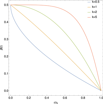
Figure 1. Velocity profile of β(r) = u(r)/c versus r/r2 for a jet shear acceleration problem. Parameter k = 0.5, 1, 2, 5 controls the u(r) profile of the jet.
Download figure:
Standard image High-resolution imageFigures 2–7 show some of the characteristics of the Green's function solution (28). Figure 2 shows a plot of Log(f0(r, p)/D) versus Log(p/p0), where the normalization constant  and the injection rate N0 is defined in (14). The figure is for a jet with β0 = 0.5, β2 = 0, and β1 = 0.25. The solution (28) is a function of r via the rapidity ξ(r), which in turn depends on the parameter k. However, the characteristics of the solution written in terms of ξ(r) or β(r) do not depend explicitly on the parameter k.

Figure 2. Log(f0/D) versus Log(p/p0) for the solution (28) for a range of values of β(r) for a jet with central velocity β0 = 0.5 and α = 1. β1 = 0.25 at the injection radius r = r1 and β2 = 0 at r = r2.
Download figure:
Standard image High-resolution imageThe locations r = 0, r = r1 and r = r2 correspond to the axis of the jet, the injection radius r1, and the outer radius of the jet (r = r2), respectively. The figure shows how the spectrum for f0(r, p) varies for different observational radial positions for β(r). The figure is analogous to Figure 2 of Webb et al. (2018a), except that  is independent of r (a more complicated radial dependence of τ(r, p) was used in Webb et al. (2018a), where
  as r → 0). The parameter α = 1 in Figure 2. The particle momentum spectrum at large momenta is a power law in p with
  (in this particular case
  ). At low momenta (0 < p < p0),
  as p → 0 (μ0 = 8 for the parameters used in above example). At high energies the spectral index is given by the formula
which corresponds to the lowest eigenfunction (n = 1) in the series (28). Here j0,1 ∼ 2.4048 is the first zero of the J0(z) Bessel function (Abramowitz & Stegun 1965, Table 9.5, p. 409). For low momenta (0 < p < p0), the power-law index μ0 is given by

The index μ0 > 0. There is a net radial outflux of particles in the region 0 < r < r1 at all momenta, except near p ≈ p0, where the flux is inward. In the region r > r1 there is a net outward diffusive flux of particles at all momenta (see Webb et al. 2018a). Figure 3 shows the dependence of the asymptotic spectral index  on the fluid velocity β0 on the jet axis, for a range of momentum dependencies of the scattering time τ (τ ∝ pα, α = 0, 1, 2). At non-relativistic flow velocities of the jet,
Thus,  as β02 → 0, implying that shear acceleration is not effective for non-relativistic laminar (non-turbulent) flows. In the opposite limit of ultra-relativistic jets (β02 → 1 and
  ) we obtain

(see also Webb et al. 2018a and similar results from Rieger & Duffy 2004a, 2004b, 2005). Thus shear acceleration is quite effective in relativistic jet shear flows.  as β02 → 1 for α = 1, which is comparable to the spectral index for particles accelerated by the first order Fermi mechanism at strong non-relativistic shocks with compression ratio rc = 4 (e.g., Axford et al. 1977; Krymsky 1977; Bell 1978a, 1978b; Blandford & Ostriker 1978).
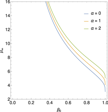
Figure 3. Asymptotic spectral index  of Equation (40) for particles accelerated in a shear flow, versus the flow speed β0 on the jet axis for a range of momentum dependencies for κ (κ ∝ pα), where α = 0, 1, 2, and for a jet with no backflow cocoon (β2 = 0). Note
  as β0 → 1, and
  as β02→0.
Download figure:
Standard image High-resolution imageFigure 4 shows the hardening of the spectrum of the accelerated particles with increasing jet velocity β0 at the source radius (r = r1) for a range of β0 (β0 = 0.3, 0.4, 0.6, 0.8, and 0.99). As the central jet velocity β0 increases, both the low energy particles with p < p0 and very-high-energy particles with p > p0 increase due to the increased diffusive spreading and systematic momentum changes.

Figure 4. Spectrum  versus Log(p/p0) at the source radius r = r1 (β = β1 = 0.1), for a range of β0 (β0 = 0.3, 0.4, 0.6, 0.8, 0.99). Here β2 = 0 and α = 1.
Download figure:
Standard image High-resolution imageFigure 5 shows Log(f0(r, p)/D) on the axis of the jet for the case β = β0 = 0.5 and α = 1 for a range of injection radii as parameterized by β1 (β1 = 0.001, 0.01, 0.2, and 0.5) and for β2 = 0 and α = 1. The smaller the value of β1, the smaller the value of f0 in Figure 5. For smaller β1, the source is located closer to the free escape boundary at r = r2, where β2 = 0, resulting in enhanced escape of particle through the free escape boundary at r = r2.

Figure 5. Spectrum Log(f0/D) versus Log(p/p0) on the axis of the jet (β = β0 = 0.5), for a range of particle injection radii (β1 = 0.001, 0.01, 0.2, and 0.5). Here β2 = 0 and α = 1.
Download figure:
Standard image High-resolution imageFigure 6 shows the variation of the spectrum f0 at the source radius (β = β1 = 0.25) for a range of diffusion coefficients with κ ∝ pα (α = 0, 0.5, 1 and 2), for the Green's function (28) with β2 = 0 and β0 = 0.5. Figure 7 shows the effect of a back-flowing cocoon for the case β0 = 0.5, β = β1 = 0.25, for a range of β2 (β2 = 0, −0.1, −0.2) and α = 1. The spectrum hardens as the net shear (as measured by β02 or β0 − β2) increases.

Figure 6. Spectrum Log(f0/D) versus Log(p/p0) at the source radius (β = β1 = 0.25) for a range of diffusion coefficients (κ ∝ pα, τ ∝ pα, α = 0, 0.5, 1 and 2) for solution (28) with β0 = 0.5 and β2 = 0.
Download figure:
Standard image High-resolution image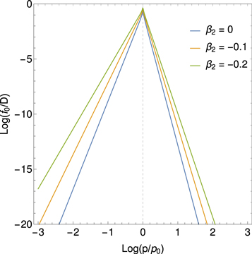
Figure 7. Log(f0/D) versus Log(p/p0). Effect of a back-flowing cocoon (β2 = 0, −0.1, and −0.2) on the solution (28) for a jet with β0 = 0.5, β = β1 = 0.25, and α = 1. The spectrum is shown at the source radius where β = β1.
Download figure:
Standard image High-resolution image4. Boundary Value Problems
4.1. The Monoenergetic Spectrum Solution
In this section we use Green's formula (Webb et al. 2018a) to solve boundary value problems for the steady-state cosmic ray transport equation:
The solution method uses the Green's functions (28) for particle transport derived in Section 3, with monoenergetic source term of the form

and f0 satisfies the boundary conditions (i) f0(r2, p) = 0 and (ii) rκ ∂f0/∂r → 0 as r → 0.
In this section we obtain the solution of (44) with Q = 0, and for a monoenergetic spectrum of particles specified on the boundary surface at r = r2 by using Green's formula. The boundary conditions for f0 are
(i.e., a monoenergetic spectrum of particles is specified on the outer boundary r = r2 of the jet).
The boundary value problem (46) for the transport Equation (44) with Q = 0 corresponds to specifying a monoenergetic spectrum of particles with momentum  at cylindrical radius r = r2 from the jet axis. The particles are accelerated and transported in the jet shear flow in the region 0 < r < r2, and eventually free escape from the acceleration region 0 < r < r2 through the boundary r = r2 (note f0(r2, p) = 0 for
  ). From Webb et al. (2018a), Equation (83) et seq., Green's formula for the transport Equation (44) gives the solution of the boundary value problem for f0(r, p) in the region:

by the formula
where  is the adjoint equation Green's function satisfying the transport equation:
and Γ satisfies the boundary conditions:
Note that the transport Equation (44) is self-adjoint (i.e.,  ). Equation (48) is Green's formula for the transport Equation (44), which gives the solution for f0(r, p) for (r, p) in
  , in terms of the adjoint Green's function, the source of particles in
  , and in terms of fluxes through the spatial and momentum boundaries.
Following Webb et al. (2018a), the solution of the boundary value problem (46) for  for a monoenergetic spectrum of particles with momentum p = p0 specified at radius r = r2 can be obtained by inserting the appropriate boundary conditions in the Green's formula (48) to obtain
as the required solution for f0(r, p). Here  in (51). In the derivation of (51), the contributions to the particle momentum fluxes through the boundaries at p' = 0 and
  are set equal to zero.
To solve the boundary value problem (46), we use the Green's function (28) to determine the adjoint Green's function  . This is achieved by using the map,

in the Green's function solution (28). These substitutions in (28) give the adjoint Green's function:
where

In (53)

and

Note that we set  and p0 → p in (29) to obtain the expression for D in (56). The diffusion coefficient
  in the map (52) is given by

Using the formulae (52)–(57) in (51) we obtain the monoenergetic spectrum solution:
where
In the derivation of (58) we used  (Abramowitz & Stegun 1965, formula 9.1.28, p. 361) in calculating the derivative of Γ with respect to r'.
4.2. Solution Characteristics
Figures 8 and 9 show some of the main characteristics of the monoenergetic spectrum solution (58) in which monoenergetic particles enter the shear flow region 0 < r < r2 with momentum p = p0 and eventually escape from the region through the free escape boundary r = r2 after being either decelerated or accelerated by their interaction with the shear flow.
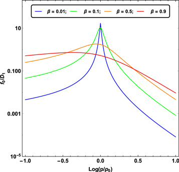
Figure 8. Particle acceleration in a jet shear flow (solution (58)) in which particles enter the shear flow at the outer boundary of the jet at radius r = r2. The central jet velocity β0 = 0.99. The momentum spectra of the particles are shown at the locations β = 0.01, 0.1, 0.5, and 0.9 (recall that β(r) is a monotonic decreasing function of r). α = 1.
Download figure:
Standard image High-resolution imageFigure 8 shows plots of the solution (58) for f0(r, p)/D1 versus Log(p/p0) for the case β0 = 0.99, β2 = 0, and α = 1. The momentum spectrum of the particles f0(r, p)/D1 are shown at different radial locations parameterized by the flow velocity β(r), which is a monotonic decreasing function of r. The spectra are shown at the locations β = 0.01, 0.1, 0.5, and 0.9. Near the edge of the jet β = 0.01 the spectrum for f0(r, p) is nearly monoenergetic. Harder momentum spectra or particles with momentum p > p0 are obtained as one moves closer to the jet axis as r decreases and β(r) increases. Both more accelerated particles and more decelerated particles are obtained as r decreases, because these particles have interacted both with the inner and outer parts of the flow. The particle momentum spectra at large p/p0 has the power-law form  , where
  corresponds to the first term in the eigen-series solution (58)—that is,
  is given by formula (40). At low momenta, the distribution function is a positive power law in momentum p with f0 ∝ pμ0 at p ≪ p0 (the expression for μ0 is given in (43)).
Figure 9 shows a similar plot of the distribution function f0(r, p) to that in Figure 8, but for the case of a jet with central velocity β0 = 0.8 and β2 = 0 at the outer boundary of the jet at radius r = r2. The parameter α = 1. The figure shows the variation in the spectra for f0(r, p) with  at p ≫ p0, and f0 ∝ pμ0 at momenta p ≪ p0. The parameter β = 0.01, 0.1, and 0.5 in Figure 9. The spectrum approaches a monoenergetic spectrum as r → r2, where β2 = 0 at the outer boundary of the acceleration region.

Figure 9. Particle acceleration in a jet shear flow (solution (58)), in which particles enter the shear flow at the outer boundary of the jet at radius r = r2. The central jet velocity β0 = 0.8. The momentum spectra of the particles are shown at the locations β = 0.01, 0.1, and 0.5 (recall that β(r) is a monotonic decreasing function of r). α = 1.
Download figure:
Standard image High-resolution image4.3. General Spectrum Solution at Jet Boundary at 


5. Energy Losses and Gains and Cosmic Ray Inertia
In general, it is difficult to include particle energy losses and gains and particle escape all together in an analytic model of particle acceleration in relativistic radio jets, without invoking some approximations and simplifications. Simplified diffusion equation models for particle acceleration in radio-jet shear flows were developed by Berezhko (1981) and Rieger & Duffy (2004a, 2004b, 2006) and Ostrowski (2002), Stawarz & Ostrowski (2002). We generalize this model to include the effects of cosmic ray inertia by using the telegrapher equation model governed by the transport equation,
in which γ is the Lorentz factor of the flow, and f0/τesc represents particle losses from the acceleration region (this model is analogous to the leaky box model used to describe galactic cosmic rays). Here Q(p, t) represents particle sources. In (63) we have assumed that the net effect of averaging the space dependent transport equation, including the telegrapher second-order time derivative term results in a transport equation with space averaged transport coefficients. The exact form of the space averaged transport coefficients must depend on the flow velocity profile of the jet about the jet axis. We do not attempt to carry out this averaging in the present paper. This makes our analysis qualitative rather than quantitative, and more work needs to be done to obtain more quantitative results.
5.1. Telegrapher Equation Effects
The first term in (63) represents a telegrapher equation term, which takes into account the finite inertia of the cosmic ray gas (e.g., Webb et al. 2018a), where

Here β = u/c and βp = v/c give the fluid speed u, and the particle speed v normalized to the speed of light. The second time derivative term in (63) limits the upper momentum pmax that takes into account the finite particle speed and inertia. In the diffusion approximation the second time derivative term is neglected. Retention of this term is important at high energies, because the diffusion approximation allows particles to attain an infinite energy in an infinitesimal time. We discuss the implications of this term in Appendix D.
In Appendix D we show that the characteristic manifold S(t, p) = const. for the second-order partial differential Equation (63) satisfies the characteristic equation

The momentum space diffusion coefficient Dpp can be split up into two terms:

where
describe stochastic particle acceleration due to cosmic ray viscosity (Dppsh) and second-order Fermi acceleration, owing to Alfvénic turbulence (Dppsf).
From Appendix D, the bi-characteristics of (63) (i.e., the characteristics of (65)) are given by the ordinary differential equation:
The maximum particle momentum pmax(t) allowed in the telegrapher Equation (63) corresponds to the σ = +1 possibility in (68). In (68) βA = VA/c is the relativistic Alfvén speed divided by the speed of light. The case σ = −1 in (68) corresponds to the minimum momentum implied by the telegrapher Equation (63).
In the formulae below we take βp = 1 corresponding to the case of fully relativistic particles only. In the more general case where the particles are not necessarily relativistic, Equation (68) can be integrated numerically if required.
For the special case of no second-order Fermi acceleration due to Alfvénic turbulence (βA = 0,  ), the σ = +1 version of (68) reduces to

Integrating (69) with initial condition p = p0 at time t = 0 gives the solution
for the maximum particle momentum due to pure shear acceleration alone. On the other hand, for the case of no shear ( ) and inclusion of second-order Fermi acceleration (
 ), (68) with σ = +1, reduces to the equation
Integration of (71) with  at time t = 0 (i.e., p = p0 at t = 0) gives the solution
for the maximum particle momentum implied by the telegrapher Equation (63) due to second-order Fermi acceleration alone.
The solution of (68) with σ = +1 for the general case ( and
and  ) is given by (198)—that is,
where

Note that (72)–(74) apply to the case  (see Appendix D for the case α = 0).
5.1.1. Lower Limits to Acceleration Timescales
It is interesting to invert the formulae (70)–(73) to give t as a function of p and p0 (i.e., t = t(p, p0)), which intuitively should give a lower time estimate for particles to be accelerated from momentum p0 up to momentum p (see, e.g., Drury 1983; Malkov & Drury 2001) for similar formulae for particles to be accelerated from momentum p0 up to momentum p in a mean time t by the first order Fermi mechanism at astrophysical shocks.
Inversion of (70) gives the formula
as a lower limit to the time for particles to be accelerated from momentum p0 up to momentum p by the viscous shear acceleration mechanism. Similarly we obtain the estimate
for the lower limit for time for particles to be accelerated from p = p0 up to momentum p solely due to second-order Fermi acceleration. More generally, inversion of (73) gives the formula
for the least time for particles to be accelerated from  up to momentum p due to both shear acceleration (
 ) and due to second-order Fermi acceleration (
 ).
).
As an application of these ideas, consider the timescale (75) for particles to be accelerated from p0 up to p in a radio-jet shear flow. Use (64) for  and note that
where u0 is the jet's central velocity and L is the width of the jet. From (75) we obtain
Noting that  , we obtain the formula
where Lkpc is the jet width in kilo-parsecs. Here we have used  and 1 year = 3.154 × 10⁷ sections. If we consider p0c = 109 eV and pc = 1018 eV (i.e., p0 = 1 GeV/c and p = 1 EeV/c, where p0 corresponds roughly to the maximum in the cosmic ray intensity spectrum jT = p2f0, and p corresponds to an energy of the order of the ankle), then the formula (80) gives
where β = u/c is the jet speed. Note in (78)–(81) that these formulae depend on our estimate that du/dr ∼ u0/L. It is interesting to compare this timescale with the light-crossing timescale tlc across the jet, namely

Thus the acceleration timescale (81) is about 100 light-crossing timescales (we assume  ). Clearly for non-relativistic jets (e.g., β = 0.01) the acceleration time is much larger than 100 tlc. The above estimates of the acceleration timescale in (80) and (81) can clearly be much greater than these estimates if particle energy losses are taken into account (especially synchrotron losses for electrons, which imply that the acceleration time t(p, p0) will be much larger in that case).
5.2. Particle Momentum Losses and Gains
In this section we discuss the particle energy losses due to synchrotron losses as well as the particle energy gains due to shear acceleration. Losses due to the inverse Compton effect have a similar forms to that for synchrotron losses, but the detailed physics is different for inverse Compton losses. The transport Equation (63) divided by the Lorentz factor of the flow (γ) gives the time evolution equation for f0 in the fixed observer's frame, in which u is the velocity of the jet along the axis of the jet. In this frame the transport Equation (63) becomes
The synchrotron losses in (83) are described by Ds and by the systematic particle momentum loss term:
where
Here m0 denotes the particle rest mass and  is the particle Lorentz factor; βp = v/c; σT is the Thomson cross-section (m0 = me for electrons and m0 = mp for protons). Formulas (85) are in cgs units. In (83)–(85) the transport equation was originally obtained using the fluid frame or the scattering frame to describe the particle momentum. Thus the magnetic field B in (83) refers to the value of B in the fluid frame. The form of the field in the jet frame can be obtained by using the Lorentz transformations between frames. If there is no electric field in the fluid frame, then
  and
and  , where the subscripts ∥ and ⊥ refer to components parallel and perpendicular to the fluid velocity u and the primed superscript 'refers to the fluid frame, or scattering frame (e.g., Misner et al. 1973).
Berezhko (1981) and Rieger & Duffy (2006) derived the Green's function solution of the transport Equation (63) with source terms Qδ (t)δ(p − p0) corresponding to impulsive monoenergetic injection of particles with momentum p = p0 into a jet shear flow, with no synchrotron losses (Ds = 0), and with no particle escape ( ). They used the solution to illustrate particle acceleration by cosmic ray viscosity in radio-jet shear flows. The mean systematic acceleration rate
  is given by
where Dpp is the momentum dispersion coefficient. Using (66) and (67), we obtain
as the systematic acceleration rates due to shear acceleration and second-order Fermi acceleration, respectively.
Consider the case where the dominant acceleration mechanism is due to cosmic ray viscosity and shear in the background plasma flow, and in which synchrotron losses is the main energy loss mechanism. In this case there will be a balance between particle energization and synchrotron losses at the momentum p = p* if

at  . Using (84) and (87) in (88), the balance condition (88) reduces to

Equation (89) can also be written as

For  , (90) has the solution
In the case 0 < α < 1, synchrotron losses dominate over particle acceleration by shear for  , but shear acceleration dominates synchrotron losses for
  . The expression for
  in (91) can also be written in the form
where

which emphasizes the role of the scattering timescale τ0, the radiation timescale τr, and the shear flow timescale τsh.
However, if α > 1, synchrotron losses are dominant below p = p* and shear acceleration dominates at p > p*. This result, at first sight appears peculiar, and may indicate that the mean free path is so long, that the diffusion approximation breaks down. It needs to be investigated in more detail (e.g., by investigating the leaky box transport Equation (63) in which both particle escape losses and particle energy gains and losses are accounted for; see the discussion in Appendix E). If one includes a second-order time derivative term in the transport Equation (63) (or its space dependent version given in Webb et al. 2018a, 2018b), then the effects of a finite cosmic ray inertia will limit the maximum momentum change rate allowed. From Section 5.1 and (69) and (70), the maximum allowed particle momentum derived from the second-order derivatives in the telegrapher equation is given by
(here we have assumed for the sake of analytical simplicity that we can take Γ as a constant, in order to capture the basic physical effects). The analog of the balance condition between synchrotron losses and shear acceleration energy gains due to cosmic ray viscosity is replaced by the equation

which implies the balance equation
Equation (96) implies that losses balance gains at the momentum:
The momentum  in (97) can also be written in the form:
Because  is the maximum allowed momentum in the telegrapher transport equation model (63), we expect that
  is required by causality. We take the break momentum p*, to be defined as
In the above analysis we have not taken into account particle losses through the spatial boundaries of the acceleration region. Also, the dispersion term  term has not been taken into account in the above simple argument.
Below, we give explicit formulae for τr and τsh, which may be used to determine  in (98) for both electrons (e) and protons (p). From (85), we obtain
for the synchrotron radiation timescales for electrons (e) and protons (p), where BμG is the magnetic field induction in microGauss (i.e., 10−6 Gauss). The shear acceleration timescale is taken as

where L is a typical length scale for the shear flow. Using (100) and (101), we obtain the formulae
as expressions for  for electrons (e) and protons (p). Note that
In the above equations, L(kpc) is the typical jet width in kilo-parsecs (e.g., Webb et al. 2018a). For a sharp gradient shear layer at the edge of the jet, τsh = u/L could be much larger than the above estimate (e.g., Ostrowski 1990, 1998, 2002).
From Webb et al. (2018a), we assume a scattering time
to describe the particle scattering in the turbulent magnetic field, based on quasi-linear theory (e.g., Jokipii 1966, 1971). In (105)

where q is the power-law spectral index for slab turbulence—that is, it is assumed that the power spectrum of magnetic field fluctuations transverse to the field has the form
where kb = 1/ℓb is the correlation scale for the turbulence. In (105)

is a parameter of order unity (see Webb et al. 2018a for more detail). From (105) we obtain
The expression (92) for  is independent of p0. Using (109) for τ0 in (92), we obtain the formula

where
In the second form for P in (111) we assume Z = 1 and

The above expression (111) for P may be written as
For the case of electrons, using (113) with α = 1/3 and q = 5/3 (corresponding to Kolmogorov turbulence with q = 5/3), setting χ = 1, and using Equation (110) gives
Comparing (114) for  with (102) for
  , we obtain
From (115) we deduce
Thus, the telegrapher equation cut-off is smaller than the Fokker–Planck, systematic acceleration cut-off for sufficiently relativistic radio jets. In other words, the telegrapher equation cut-off  should be used for fast enough jets for which the inequality (116) applies. This constraint is fairly severe if we take for example ℓb/L = 0.1, in which case condition (116) reduces to

6. Summary and Discussion
In this paper, we have revisited the problem of acceleration of UHECR in relativistic jet shear flows, extending the earlier work of Webb (1990) and Webb et al. (2018a), based on the relativistic diffusive transport equation of Webb (1989). The model assumes a relativistic jet shear flow of the form  along the axis of the jet (the z-axis), in which u(r) is a monotonic decreasing function of cylindrical radius r about the jet axis (i.e., du/dr < 0). The particles are accelerated by elastically scattering in the local fluid frame, and by scattering across the jet shear flow. The particles are assumed to be relativistic for which the particle speed v ≈ c, where c is the speed of light. The mean scattering time τ(r, p) for particles with momentum p at cylindrical radius r is assumed to have the functional form
where g(ξ) is a given function of the jet rapidity,
is relativistic β of the flow and c is the speed of light. The monoenergetic source Green's function of the steady-state transport equation obtained by Webb (1990) and Webb et al. (2018a) assumed that g(ξ) was constant. This lead to solutions of the transport equation that have the property  as r → 0 for most models of the shear flow. In this paper we have explored more general choices of g(ξ) chosen, so that
We explored in detail Green's function solutions and monoenergetic spectrum solutions for the case δ = 1, in which the eigenfunction solutions for the Green's function involves zeroth order Bessel functions J0(λη), where η = η(r) depends only on the radial profile of the jet speed u(r). There are in fact other Bessel eigenfunction series Green's functions that can be obtained for cases where δ > 1 (see Appendix B for further details).
The solution examples (Figures 1–8) are very similar to those presented in Webb et al. (2018a). This illustrates that the solution details do not depend strongly on the detailed behavior of the mean scattering time τ(r, p) on the axis of the jet as r → 0 (in Webb et al. 2018a,  as r → 0, but in the present model
  does not depend on r). For an ultra-relativistic jet, the spectral index of shear accelerated particles (
 ),
),  , and in the non-relativistic limit β0 → 0,
  , where β02 is the relative velocity of β0 and β2 and j0,1 is the first zero of the ordinary Bessel function of order zero J0(z) (j0,1 ∼ 2.4048). The spectral index
  is displayed as a function of β0 in Figure 3 (see also Rieger & Duffy 2006, for discussion of the spectral index of particles accelerated in shear flows by cosmic ray viscosity). For α = 1,
  as β0 → 1, which is similar to the spectral index of cosmic rays accelerated by the first order Fermi mechanism in astrophysical shocks (Axford et al. 1977; Krymsky 1977; Bell 1978a, 1978b; Blandford & Ostriker 1978). Allowing for a back-flowing cocoon with an increased overall shear of the flow leads to harder particle spectra.
In Section 3, steady-state Green's function solutions of the relativistic diffusive transport equation (Webb 1989) were obtained for a cylindrically symmetric jet in which the flow velocity u = u(r) ez. The Green's function consists of an eigenfunction expansion in terms of J0(λnη) Bessel functions where η = η(r) describes the radial dependence of the solution and the λn are eigenvalues. The Green's function corresponds to steady injection of particles with momentum p = p0 at radius r = r1 from the jet axis, with free escape boundary conditions at radius r = r2 (r2 > r1). The flow profile u(r) is determined in part by requiring the mean scattering time τ(r, p) to be independent of r (i.e.,  ).
).
Green's formula for the transport equation was obtained in Section 4. It gives the solution of boundary problems for f0(r, p) in terms of the Green's functions of Section 3, and in terms of the boundary and initial data. In particular, the Green's formula gives solutions of boundary value problems in which a spectrum of particles is specified at the outer boundary of the jet at r = r2 and in terms of sources of particles inside the jet at radii 0 < r < r2. The Green's formula was used to obtain monoenergetic spectrum solutions in which  as r → r2, and with no sources inside the jet shear flow region 0 < r < r2. In these solutions there is a radial influx of particles with momentum p = p0 and an outflux of particles at higher and lower momenta that have either have been accelerated (p > p0) or decelerated (p < p0) by their interaction with the shear flow.
Astrophysical applications of the model to the acceleration of UHECR to ultra-high energies in extragalactic radio jets were discussed in Liu et al. (2017) and Webb et al. (2018a). Constraints on the acceleration mechanism were used to delimit the width  of the radio jet and magnetic field strength B needed to constrain and accelerate E = 1018 eV protons in the jet, taking into account proton synchrotron losses and other constraints (e.g., the width of the jet ΔL needs to be greater than the particle mean free path λ in order that the particles are confined to the jet and can interact with the shear flow; the particle acceleration time needs to be less than the dynamical advection time in order for the particles to be accelerated by the shear before being advected out of the region). Equation (99) of Webb et al. (2018a) gives a formula for the gyro-radius of the particles that is too big by a factor of about 10. Correcting for this error results in estimates for the allowed jet width to be approximately one tenth of those given in Webb et al. (2018a). These corrections to (99) et seq. of Webb et al. (2018a) are discussed in detail in Appendix F. Constraints on ΔL and B for the case of isotropic diffusion from Webb et al. (2018a; adjusted for the above error) for particles with E = 1018 eV (i.e., 1 EeV particles), are 1 kpc < ΔL < 105 kpc for B =1 μG and 10 pc < ΔL < 103 kpc for B = 100 μG for a radio jet with a Lorentz factor γj = 1.1 (βj = 0.4166). The length of the jet d = 100 ΔL was assumed. AGN jets of these approximate size and magnetic field constraints (Liu et al. 2017 and Webb et al. 2018a) imply that the sources MKN 501 and MKN 421; Dermer (2007), Sahayanathan (2009), Abbasi et al. (2014), Caprioli (2015) are possible sources of EeV protons accelerated by the cosmic ray viscous shear acceleration mechanism.
In Appendix C we discuss how the analysis is altered by assuming that the particles have a finite diffusion coefficient in the region r > r2, but there is no particle acceleration by shear in the region r > r2 outside the jet. Assuming that that there is a spectrum of particles  as
as  and that there are no sources of particles, in r > r2, the boundary condition at r = r2 reduces to the equation
Effectively the solutions of Section 4, in which f0(r2, p) are specified on a free escape boundary at r = r2, assume that  in r > r2. More precisely, if κ ∝ pαrs in r > r2, the boundary condition (121) reduces to the equation

The boundary condition (122) is a mixed Dirichlet–Von Neumann boundary condition. For s ≫ 1 (122) is approximately the Dirichlet boundary condition:

which is essentially the free escape boundary condition used in Section 4. The effect of including a finite κ in r > r2 will result in a harder spectrum of accelerated particles in r < r2 because there is a finite probability that the particles leaving the acceleration region (r < r2) will return to the region r < r2 to be further accelerated by the shear flow. This is an interesting extension of the solutions presented in Sections 3 and 4, which lies beyond the scope of the present paper.
Section 5 discusses the effect of energy losses and particle escape from the acceleration region by using a leaky box type transport equation, including the effects of cosmic ray inertia, momentum space diffusion energy changes due to shear acceleration, and second-order Fermi acceleration due to Alfvén waves. From an analysis of the characteristic manifold and bi-characteristics of a telegrapher type transport equation we obtain a first order ordinary differential equation for p = p(t), which gives the maximum possible momentum of the particles in the model. It is shown in Appendix D that if one uses a diffusion equation analysis to calculate the mean particle momentum  for the particle acceleration, one obtains a contradictory result that particles can be accelerated to an infinite momentum in a finite time. This non-physical result can be circumvented by including a second-order time derivative term in a telegrapher type transport equation that incorporates the effect of the cosmic ray inertia. Appendix E discusses a steady-state leaky box model for particle acceleration due to cosmic ray viscosity in the presence of synchrotron losses, and in particular we discuss the dependence of the solution on the momentum dependence of the particle scattering time
  through the parameter α, for the separate cases (a) 0 < α < 1, (b) α = 1 (Bohm diffusion), and (c) α > 1.
As an application of the pmax(t) formula implied by the telegrapher equation, we estimate a lower limit to the time for particles to be accelerated in a radio-jet shear flow, with a typical width of L ∼ 1 kpc in which the particles are injected with a momentum p0 = 1 GeV/c and obtain a momentum of p = 1 EeV/c on a timescale of the order of 105–106 yr for a mildly relativistic jet. The estimate of pmax(t) based on the telegrapher equation bi-characteristics in the example turns out to be about 100 light-crossing times of the width of the jet. The analysis assumes that the transport Equation (63) has space averaged transport coefficients of the same form as the space dependent transport equation (e.g., Webb et al. 2018a, Appendix E). The averaged transport coefficients depend on the details of the model parameters for the jet.
Estimates of acceleration times (based on the telegrapher equation bi-characteristics, and also on the Fokker–Planck mean drift momentum term) are used to investigate if the particle momentum losses balance the momentum gains at some critical momentum p = p* in which the particle energy losses exceed the momentum gains at momenta p > p*, in which case there is a break in the momentum spectrum and a fall off of the particle momentum spectrum at p > p*. In fact if there is very strong particle acceleration, then there can occur a momentum pile up in the spectrum due to strong deceleration of particles above p* and strong acceleration below p* (e.g., Kardashev 1962). Kardashev (1962) studies a variety of energy loss mechanisms (synchrotron losses, expansion losses, nuclear losses, Bremsstrahlung losses, ionization losses, and inverse Compton losses) and stochastic acceleration of the particles, with application to a variety of sources (e.g., the Crab Nebula, SNR Cass A, Jet in NGC 4486, Cygnus A). Similar ideas have been used to describe diffusive shock acceleration of electrons subject to synchrotron losses in astrophysical shocks (e.g., Webb et al. 1984; Fritz & Webb 1990; Blasi 2010). We find that for sufficiently relativistic flows, if the balance point in momentum, based on the telegrapher equation approach for the balance or break point in the spectrum  , is less than the cut-off based on the diffusive transport equation,
  , then the solution effectively must cut off at
  and not at
  , as assumed in earlier analyses.
It was pointed out by Webb et al. (2018a) that time-dependent, diffusive transport equations for the acceleration of particles involving second-order momentum diffusion are non-causal, as they predict that particles can attain an infinite energy in a finite time. These defects of diffusive transport equations can be partially overcome by generalizing the diffusive transport equation to include a second-order time derivative term representing cosmic ray inertia (e.g., Fisk & Axford 1969) to obtain a telegrapher equation for cosmic ray transport. Analysis of the telegrapher equation characteristic manifolds and bi-characteristics suggests the formula (Webb et al. 2018a):
for the maximum particle momentum for particles accelerated by the cosmic ray viscous shear acceleration mechanism in the relativistic jet shear flow for particles injected into the flow with momentum p = p0 at radius r = r0 at time t = 0. Here  is the cosmic ray sound speed for isotropic relativistic particles (e.g., Webb 1987a; Kirk & Webb 1988);
  , where γ is the relativistic Lorentz factor of the flow. For simplicity, β, γ, and Γ were assumed constant when integrating the bi-characteristics (numerical integration of the bi-characteristics could in principle be used to obtain more accurate estimates of pmax). A preliminary account of these ideas was presented in Webb et al. (2018a) and in a poster paper at the fall AGU meeting in 2018 December (Webb et al. 2018b). We hope to address some of these issues in more detail in future publications.
G.M.W. acknowledges discussions with Frank Rieger, who pointed out the numerical error in the expression for the particle gyro-radius in Equation (99) of Webb et al. (2018a). We thank the referee for a very thorough report and for pointing out inconsistencies and errors in the original manuscript. G.M.W. and G.L. were supported in part by NASA grant 80NSSC19K0075. P.M. acknowledges the support of a NASA Earth and Space Science Fellowship Grant 16-HELIO16F-0022. J.A.L.R. is supported in part by NASA grants NNX15A165G, 80NSSC19K0276, and NSF-DOE grant PHY-1707247. G.P.Z. has been supported in part by the NSF EPSCoR RII-Track-1 Cooperative Agreement OIA-1655280 and an NSF/DOE Partnership in Basic Plasma Science and Engineering via NSF grant PHY-1707247. A.F.B. acknowledges valuable insights and discussions with Prof. Peter Biermann on UHECR and candidate sources and radio galaxies.
Appendix A
In this appendix we derive the Green's function solution (28) of the steady-state transport Equation (26), including the effects of particle acceleration due to cosmic ray viscosity and fluid shear. We derive the Green's function by two different methods. The first method uses the Fourier transform of the partial differential Equation (26) with respect to T. The second method uses a Fourier–Bessel expansion consisting of separated solutions of (26), which take into account the Delta function source term in (26), in which the Delta function  is expanded in terms of the Bessel equation eigenfunctions for the problem.
A.1. Fourier Transform Approach
We introduce the Fourier transform with respect to T in the form:

Taking the Fourier transform of (26) with respect to T gives the ordinary differential equation,
where
Notice that
The homogeneous Equation (126) has solutions of the form

where η = ξ0 − ξ, and I0(z) and K0(z) are modified Bessel functions of the first and second kind of order zero (Abramowitz & Stegun 1965, 9.6.1, p. 374). The general solution of the inhomogeneous ordinary differential Equation (126) is given by the general formula
(Morse & Feshbach 1953, Vol. 1, p. 530, 5.2.19), where Wη(y1, y2) = y1dy2/dη − y2dy1/dη is the Wronskian of the two independent solutions y1 and y2 of the homogeneous Equation (126), which are listed in (129). In (128) and (129) we use the Re(Λ) > 0 branch of the multi-valued function Λ, and we use the variable  rather than ν in the analysis.
Using the properties of I0(z) and K0(z) to fit the boundary conditions as r → 0 and as r → r2, we obtain the solution for  in the form
where

The required solution for f0(r, p) is obtained by using the inverse Fourier transform formula:

To carry out the inverse Fourier transform (134), it is useful to note that  has simple poles in the complex λ-plane at points where

These poles occur at the points
where  is the nth zero of J0(z)—that is,
  (n a positive integer). The value of ν' = ν + ia at these points are given by

The multi-valued complex function Λ = Λ(ν') is chosen to have a branch cut from ν' = ia to  along the Im(ν') > 0 axis, and also a cut from ν' = −ia to
  along the Im(ν') < 0 axis. It turns out that the transform (131) does not jump in value (i.e., is continuous) across the branch cut.
Using standard complex variable theory (i..e. Cauchy's theorem) to invert the solution (131) for  gives the Green's function solution for f0(r, p) in the form
where
The solution (138) is equivalent to the solution (28). To show that (138) is equivalent to (28), note that the Wronskian  of J0(z) and Y0(z) is given by

(Abramowitz & Stegun 1965, formula 9.1.60, p. 360). Also note that

(Abramowitz & Stegun 1965, formula 9.1.28, p. 361). Using (140) and (141) with z = j0,n, we obtain

which implies
Using the result (143) in (138), the solution (138) reduces to the Green's function (28).
A.2. Fourier–Bessel Series Approach
An alternative derivation of the Green's function (28) (e.g., Webb & Gleeson 1977) is to first note that the problem has a discrete i.e., countable eigenspectrum {λn}, where λn = j0,n/η2 and the j0,n are the zeros of J0(x). This spectrum arises because we impose the boundary condition that f0(r2, p) = 0 at r = r2 and impose a regularity condition on the particle diffusive flux as r → 0. The transport Equation (26) admits separable solutions of the form

where hn(T) is to be determined.
To determine hn(T), first note that we can write

which is a Fourier–Bessel expansion for δ(η − η1). By using Bessel's equation, we obtain the relations

where
Here Wmn is the Wronskian of gm(η) and gn(η). From (146) to (147), we obtain the orthogonality relations for the {gn(η)} eigenfunctions—namely,

where δmn is the Kronecker delta symbol and
are the normalization constants.
To determine the cn, multiply (145) by ηJ0(λmη) and integrate over η from η = 0 to η = η2, using (148). This gives

for the constants {cn} in (145). Next we substitute the eigenfunction expansion (144) into the transport Equation (26) and use the Delta function representation (145) for δ(η − η1) in the source term in (26). We obtain the equation

for the hn(T). Here we have written the source term in (26) in the form −Aδ(T)δ(η − η1), where
The homogeneous Equation (151) has independent solutions,

With Wronskian,

Using the general formula (130) to solve the inhomogeneous Equation (151) and requiring hn(T) to be bounded as  , we obtain the required solution of (151) in the form:
Substituting the solution (155) for hn(T) in (144) and using (152) for A, and (149) and (150) for the cn, the solution (144) reduces to the Green's function (28).
Appendix B
In this appendix, we indicate how the Bessel function eigenfunction expansion for the steady-state Green's function (28) can be generalized for other choices of the function g(ξ) used to define the mean free time τ(r, p) in (1) and (20). In particular, we consider the family of solutions of the transport Equation (21) that are obtained by choosing

and by choosing

The solutions in Sections 3 and 4 correspond to the choice δ = 1 in (156) and (157) (see also Appendix A).
From (156) and (157), we obtain the differential equation

To integrate (158), we use the auxiliary variable

where ξ0 = ξ(0). We consider solutions with η > 0 so that dξ/dr < 0, and ξ(r) is then a monotonic decreasing function of r. Integration of (157), by setting ξ2 = ξ(r2), results in the solution of (158) as
where we assume  . For the above solution,

is a monotonic decreasing function of r.
Using the form (156) for g(ξ) in the transport Equation (21) results in the equation
The homogeneous partial differential Equation (162) admits separated solutions of the form

where c and d are arbitrary constants, and Jm(z) and Ym(z) are Bessel functions of the first and second kind of order m, where

It is clear from the separated solutions (163) that steady-state Green's functions of (162) can be constructed using the separated solutions (163), following the approach of Appendix A. In particular we obtain the Green's function analogous to (28) in the form
where Jm(z) are ordinary Bessel functions of the first kind of order m, and the eigenvalues {λn} are the positive zeros of the eigenvalue equation
where the {jm,n} are the positive zeros of Jm(z)—that is, Jm(jm,n) = 0 for n = 1,2,3, .... In (165),
The solution (165) reduces to the solution (28) in the limit as m → 0. Second, as  , the solution (165) has the asymptotic spectrum
  , where

This spectral index is larger than the spectral index  given by (40). This indicates that the flow profile (167) for β(r) for
  is less efficient for accelerating particles than the case for m = 0. The detailed properties of the solution (165) for
  will not be explored further in the present paper.
Appendix C
In this appendix, we discuss a modified boundary condition to apply to the particle momentum spectrum f0(r, p) and ∂f0/∂r at the edge of the jet at cylindrical radius r = r2. The boundary condition used in (46) was that f0(r2, p) is specified at the edge of the jet at r = r2. This boundary condition does not explicitly address the particle transport in the region r > r2. It could be interpreted as the solution of the transport Equation (44), with  in r > r2.
However, if one assumes there is no particle acceleration in r > r2, but the diffusion coefficient is given in r > r2, then the particle transport Equation (44) in r > r2 reduces to
where for simplicity we assume that Q(r, p) = 0 in r > r2. The solution of (169) in r > r2 has the form
where C(p) and D(p) are "integration constants," and we assume that the integral in (170) is finite. Note that

is a first integral of (169). From (171), it follows that

may be identified as the diffusive particle flux at r = r2.
Letting  in solution (170), we obtain
for the unknown function D(p). Using (172) and (173) for C(p) and D(p), we obtain the solution for f0(r, p) in  as
as
Setting r = r2 in (174) gives the boundary condition at r = r2 as
In order to get a better feel for the implications of the boundary condition (175) consider the case where
Using (176) in (174), we obtain

for f0 in r > r2.
The boundary condition (175) then becomes

The boundary condition (178) is a mixed Dirichlet–Von Neumann boundary condition. For s ≫ 1, (178) is approximately the Dirichlet boundary condition:

which is the free escape boundary condition used in Section 4. In the opposite limit (s → 0), the boundary condition (178) reduces to an approximate Neumann boundary condition:

The detailed application of the boundary condition (178) to particle acceleration in radio-jet shear flows lies beyond the scope of the present paper. Intuitively we expect that the boundary condition (175) or (178) will lead to harder particle spectra, because particles crossing r = r2 into the region r > r2 may now return back into the region r < r2 to be further accelerated by the shear flow inside r = r2.
It is clear that one could also include a source term  on the right-hand side of (169). Similarly, one could include sources of particles in the region 0 < r < r2 in the problem.
Appendix D
In this appendix we derive formulas for the maximum particle momentum, based on the characteristic classification of the telegrapher transport Equation (63). A similar discussion of the telegrapher equation, including spatial diffusion, was given in Appendix E of Webb et al. (2018a). The basic, space averaged transport Equation (63) may be written in the form
In (181)
where  and βp = v/c are the fluid speed (β) and the particle speed (βp) normalized to the speed of light. The characteristic manifold of the partial differential Equation (181) is the manifold S(t, p) = const. on which the Cauchy initial value problem for (181) does not have a unique solution. The function S(t, p) (sometimes referred to as the wave eikonal function in JWKB theory) satisfies the first order partial differential equation:

(e.g., Sneddon 1957; Courant & Hilbert 1989). Note that (183) arises when one tries to calculate higher order derivatives from lower order derivatives by using the partial differential equation and new coordinates ξ(t, p) and η(t, p) to replace t and p as independent coordinates. If the determinant of the transformation from the old coordinates (t, p) to the new coordinates (ξ, η) is zero, then it is not possible to obtain a unique solution (ξ and η can be identified with the possible solutions for S, which in the present case satisfy (183)). Note that ω = −St and k = Sp in (183) can be thought of as the frequency ω and wave number k that result from solving the wave equation implicit in (181) which consists of the second derivative terms in (181).
The momentum diffusion coefficient Dpp in (183) due to both cosmic ray viscosity and due to second-order Fermi acceleration arising from Alfvénic turbulence is given by
where βA = VA/c is the ratio of the Alfvén speed to the speed of light (we require VA/c < 1, which means VA is the relativistic Alfvén speed). The term  is the second-order Fermi acceleration coefficient due to Alfvén waves (e.g., Skilling 1975).
Using (183)–(184), we write (183) in the form
where

Consider the characteristic equation

The characteristics for (187) (the so-called bi-characteristics of (181)) are given by
where χ is the affine parameter (or distance parameter) along the characteristic (e.g., Sneddon 1957). From (188) we obtain the differential equation,
for the maximum particle momentum in the telegrapher Equation (181), where we have assumed the mean free time τ(p) has the form

At this point, we could integrate (189) directly to obtain the maximum particle momentum p = pmax(t) for particles initially with momentum p = p0, as predicted by the telegrapher Equation (181). For analytical simplicity, we restrict the analysis below to relativistic particles for which βp ≈ 1. It is clear that (189) can be integrated for general βp if necessary by numerical integration. In the analysis below we consider only the case of relativistic particles in which we set βp = 1. We prefer here to illustrate the solutions of (189) for relativistic particles (βp = 1) for the special cases (i) βA = 0 and  (pure viscous acceleration case) and (ii)
  and Γ = 0 (pure second-order Fermi case). In case (i)
Integration of (191) with respect to t, with initial condition p = p0 at time t = 0, gives the solution
for the maximum particle momentum due to pure shear acceleration alone. Similarly, in case (ii), (189) reduces to the equation
Integration of (193) with  at time t = 0 (i.e., p = p0 at t = 0) gives the solution
for the maximum particle momentum, where we assume  . For the case α = 0, we obtain the solution
Equations (194) and (195) give the maximum particle momentum for the case of pure second-order Fermi acceleration (i.e., case (ii)).
Comparing the solutions (192)–(195), we see that the solutions for second-order Fermi acceleration and no shear (Equations (194) and (195)) depend on the scattering time τ0, but the pure shear acceleration solution (192) does not depend on τ0.
Finally, we note that integration of (189) for the general case where  and
and  and βp = 1, satisfying p = p0 at t = 0 may be written in the form

where

From (196) we obtain
as the general solution for the maximum particle momentum p(t) allowed by the telegrapher Equation (181), including both second-order Fermi acceleration ( ) and viscous shear acceleration (
 ) where
  . For the case α = 0, (189) simplifies to
Integration of (199) with p = p0 at t = 0 gives the solution
where Γ* in (199) contains both shear acceleration (Γ) and second-order Fermi ( ) terms.
D.1. An Anomaly for

If one uses the mean acceleration rate for shear acceleration in (87) and integrates the differential equation
with p = p0 at t = 0, one obtains the solution for p as

Alternatively, the solution (202) can be expressed in the form

The result (204) is clearly non-physical, as it implies that particles can be accelerated to an infinite momentum in a finite time. This non-causal behavior is a result of neglecting the finite inertia of the cosmic rays (i.e., the telegrapher second-order time derivative term in (181)).
One can obtain solutions of the characteristic Equation (185) corresponding to the solution branch G− = 0. This in general gives a lower momentum pmin(t) implicit in the solution of (181). However, it turns out in the case of second-order Fermi acceleration that the minimum momentum pmin can be negative, which of course is not physically acceptable. Also note that the coefficient of f0,tt in (181) tends to zero as p → 0, suggesting that the f0,tt term should be neglected at small p (assuming τ ∝ pα with α > 0).
Appendix E
In this appendix we investigate the steady-state leaky box model (63) for particle acceleration due to cosmic ray viscosity in the presence of synchrotron losses and particle escape. We concentrate on the case where  and Q = 0.
The steady-state transport Equation (63) with Q = 0 has the form
We consider the simplest case where the escape time  (i.e., there is no particle escape from the box). Here

Equation (205) with  integrates to give the first integral,

where C0 is the integration constant, and where for the sake of simplicity we take Γ to be a constant. Equation (207) can be written in the form
where we use the notation  to denote the function f0(p) in terms of the normalized momentum
  .
.
The integrating factor for Equation (208) depends on whether α = 1 or  . For
. For  , the integrating factor
  is
is
where
is a dimensionless parameter that measures the relative importance of synchrotron losses to shear acceleration due to cosmic ray viscosity. For α = 1 (Bohm diffusion case), we obtain

for the integrating factor  .
.
The general solution of (208) using the integrating factor (209) is
where C1 is a second integration constant. In (208)–(212) we identify the constants C1 and C0 for  as
as
For the case α = 1, C1 = f0(p0) and C0 are given by (213). Thus, in general,  and
and  .
.
For the case of Bohm diffusion (α = 1), the solution (212) reduces to the simple form

where
The first term in (214) represents pure synchrotron losses. It dominates the solution for p ≫ p0 if χ > 4. The second term in (214) represents the competition between synchrotron losses and particle acceleration due to cosmic ray viscosity. It dominates the solution at large momenta p ≫ p0 in the case where 0 < χ < 4 (this is the case of dominant particle acceleration due to cosmic ray viscosity), resulting in  as
as  .
.
For the case 0 < α < 1, the solution (212) for p ≫ p0 can be approximated by
where

Equation (216) shows that for  the pure synchrotron spectrum dominates the shear viscosity acceleration process as
  . This result agrees with the results of (90), where synchrotron losses beat shear acceleration gains at
  . The result (216) follows from an analysis of the second term in (212), namely

and by using Laplace's asymptotic method to evaluate the integral (218) for large values of the parameter w. To evaluate (218) for large w, note that  , so that
and then consecutively use the integration variables

followed by the use of Laplaces's method using integration by parts to asymptotically evaluate  for the case where χw is a large parameter (we omit the details). The net result is the asymptotic solution (216) for f0 for large p.
Similarly, for the case α > 1, the solution (212) for f0 may be written in the form
where

Here
The integrals (223) can be expressed in terms of the incomplete Gamma function γ (a, x):

(Abramowitz & Stegun 1965, p. 260, formula 6.5.2). We find
Note from (209), the integrating factor  as
as  . Because we require
  as
as  , we set
as a relationship between C1 and C0 required for the physical solution. Using (226), the solution for  in (221) reduces to
Using the expansion
(Abramowitz & Stegun 1965, p. 260, formula 6.5.29), the solution (227) for  reduces to the form
where

The asymptotic formula for f0 as  in (229) is that expected from particle acceleration in shear flows in the absence of losses (e.g., Berezhko & Krymsky 1981; Rieger & Duffy 2006). This agrees with the analysis of (90), in which particle acceleration by shear dominates the synchrotron losses at
  for the case α > 1.
If we assume a finite escape time τesc(p) in (205), then we expect f0 → 0 as  for τesc, a sufficiently fast increasing function of p. If one assumes an escape time

in the leaky box transport Equation (205), and assuming Γ can be taken as a constant, (205) reduces to the second-order ordinary differential equation
For the case  , the transformation of variables,

transforms the ordinary differential Equation (232) to the confluent hypergeometric equation
which has the general solution
Here a1 and a2 are arbitrary constants and M(a, b, y) and U(a, b, y) are independent solutions of the Kummer's confluent hypergeometric equation (e.g., Abramowitz & Stegun 1965, Ch. 13, p.504). The solutions (235) could have been used to carry out the asymptotics of the solutions for  for
for  . Further analysis of (232) for a finite escape time τe0 is an interesting problem, which lies beyond the scope of the present paper.
Appendix F
Here we correct the formula for rgp of (99) of Webb et al. (2018a), and correct other Equations in (99) et seq. of that paper. The corrected rgp is
Condition ΔL > rgp/η, for particle confinement by the jet in Webb et al. (2018a) (103), reduces to
Webb et al. (2018a) (107) for the acceleration time tacc becomes
Formula (106) for the synchrotron loss time remains the same as in Webb et al. (2018a). Condition tacc < tsynch for particles to be accelerated despite synchrotron losses reduces to the condition
Assuming that  (ρw = 0.01), the condition tacc < tdyn = d/(cβj) (i.e., the corrected (109) of Webb et al. 2018a) gives the constraint
These equations delimit the  and B regions in which the E = 1EeV particles are confined during acceleration in radio jet and correct (99) et seq. of Webb et al. (2018a).
Figures 10 and 11 (the corrected Figure 10 and 11 of Webb et al. 2018a) illustrate the three constraints (i) ΔL > rgp (237) with η = 1, (ii) the acceleration time tacc < tsynch (239), and (iii) the acceleration time tacc < tdyn (240). The allowed ΔL and B(μG) regions are shown by the gray-shaded regions.
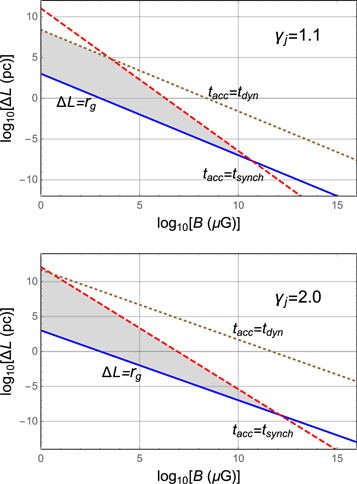
Figure 10. Constraints (237), (239), and (240) on E = 1018 eV protons acceleration in radio jets for the cases (a) γj = 1.1 (top panel) and (b) γj = 2 (bottom panel), where  ,
,  (isotropic diffusion), q = 5/3, β2 = 0, and ρw = 0.01 for a wide range of jet radii ΔL and magnetic field strengths B. The allowed region of phase space of ΔL and B is shaded in gray.
Download figure:
Standard image High-resolution image
Figure 11. Constraints (237), (239), and (240) on E = 1018 eV protons acceleration in radio jets for the cases (a) γj = 1.1 (top panel) and (b) γj = 2 (bottom panel), where η = χ = 1,  (i.e., anisotropic diffusion with
  ), q = 5/3, β2 = 0, and ρw = 0.01 for a wide range of jet radii ΔL and magnetic field strengths B. The allowed region of phase space of ΔL and B is shaded in gray.
Download figure:
Standard image High-resolution image