


Abstract
Recent studies of unusual or atypical energetic particle flux events (AEPEs) observed at 1 au show that another mechanism, different from diffusive shock acceleration, can energize particles locally in the solar wind. The mechanism proposed by Zank et al. is based on the stochastic energization of charged particles in regions filled with numerous small-scale magnetic islands (SMIs) dynamically contracting or merging and experiencing multiple magnetic reconnection in the super-Alfvénic solar wind flow. A first- and second-order Fermi mechanism results from compression-induced changes in the shape of SMIs and their developing dynamics. Charged particles can also be accelerated by the formation of antireconnection electric fields. Observations show that both processes often coexist in the solar wind. The occurrence of SMIs depends on the presence of strong current sheets like the heliospheric current sheet (HCS), and related AEPEs are found to occur within magnetic cavities formed by stream–stream, stream–HCS, or HCS–shock interactions that are filled with SMIs. Previous case studies comparing observations with theoretical predictions were qualitative. Here we present quantitative theoretical predictions of AEPEs based on several events, including a detailed analysis of the corresponding observations. The study illustrates the necessity of accounting for local processes of particle acceleration in the solar wind.
Export citation and abstract BibTeX RIS
1. Introduction
Charged particles with energies up to several tens of MeV observed at the Earth's orbit are generally supposed to be of solar origin. Solar energetic particles (SEPs) are thought to be accelerated either during the evolution of solar flares or at shocks driven by interplanetary coronal mass ejections (ICMEs) (Lee & Ryan 1986; Reames 1990; Zank et al. 2000, 2006; Li et al. 2003; Rice et al. 2003). Interplanetary shocks (ISs) effectively energize charged particles in the solar corona via diffusive shock acceleration (DSA) (Klein et al. 1999; Mann et al. 2003; Lee 2005). In addition to particle acceleration by ICME-driven ISs, other forms of ISs are also thought to be responsible for particle acceleration beyond 1 au. For example, a pair of forward-reverse ISs formed at 2–3 au on the borders of long-lived corotating interaction regions (CIRs) or less stable transient stream interaction regions (SIRs) also energize energetic particles up to several MeV in the quiet solar wind (Forsyth & Gosling 2001; Malandraki et al. 2007; Tsubouchi 2014).
It has long been regarded that DSA is the only process capable of accelerating particles to substantial energies directly in the solar wind (Drury 1983; Zank et al. 2007). However, recent in situ observations and theoretical models suggest that other mechanisms, which have been underestimated considerably, may also lead to local particle acceleration in the heliosphere (Zank et al. 2014, 2015; Khabarova et al. 2015, 2016, 2017, 2018a; le Roux et al. 2015, 2016; Khabarova & Zank 2017). Energetic particle flux enhancements up to several MeV that cannot be attributed to the shock-related sources are observed in the vicinity of the heliospheric current sheet (HCS). The particle flux enhancements are often detected many hours prior to the arrival of CIRs, sometimes within the main body of ICMEs, and sometimes there is simply no association with any obvious source. Such energetic particle flux enhancements are described as atypical energetic particle events (AEPEs) (Khabarova et al. 2015, 2016). Regions related to AEPEs are observed by different spacecraft with a time delay that corresponds to the propagation of the low-energy solar wind from one point to another and thus reflects the local origin of AEPEs.
Khabarova et al. (2015, 2016, 2017, 2018a) summarized prior observations of AEPEs and provided evidence for the presence of magnetic islands in magnetically confined regions that are apparently responsible for the observed particle acceleration. Khabarova et al. (2015, 2016, 2017, 2018a) established a link between AEPEs and local magnetic flux ropes or magnetic islands. Khabarova & Zank (2017) took a further step forward, confirming the local character of particle acceleration and comparing qualitatively theoretical predictions and observations.
To understand the nature of AEPEs requires a focused investigation taking a comprehensive approach in which events are simultaneously considered both observationally and theoretically. We show below that AEPEs are determined by magnetic reconnection–associated processes that may occur in quite different types of solar wind plasma. The key feature necessary to ensure the local acceleration of energetic particles is the occurrence of dynamical coherent structures confined by strong current sheets (SCSs) such as the HCS.
Coherent structures represented by current sheets, flux ropes, and/or magnetic islands and discontinuities of various scales can be produced by both turbulence and large- or small-scale turbulent magnetic reconnection (Dmitruk et al. 2004; Eriksson et al. 2009; Servidio et al. 2009, 2010, 2011; Moore et al. 2013; Khabarova et al. 2015, 2016; Khabarova & Zank 2017; Zank et al. 2017; Zheng & Hu 2018). It is known that reconnecting current sheets in the solar wind are surrounded by waves, secondary current sheets, and small-scale magnetic islands (SMIs) (Cartwright & Moldwin 2010; Khabarova & Zastenker 2011; Eriksson et al. 2014). In an ensemble-averaged sense, this is indeed a signature of fully developed turbulence in the plasma-β ∼1 or ≪1 regime (Zank et al. 2017). Dynamical processes in SMIs produce a cascade of smaller-scale current sheets. Magnetic reconnection, a dissipative process associated with the nonlinear cascade, is therefore ubiquitous in a turbulent magnetized plasma. Also, within a confined region of magnetic cavities, neighboring SMIs of the same chirality attract each other due to the Lorentz force and may create numerous SMIs and current sheets of smaller scales (Greco et al. 2008, 2009a, 2009b; Servidio et al. 2009, 2010, 2011; Zank et al. 2017). A statistical analysis by Osman et al. (2014) and wavelet analysis by Lion et al. (2016) confirm that the turbulent solar wind is characterized by a hierarchy of intermittent turbulence associated with current sheets and magnetic reconnection. Many properties of the dynamical turbulent solar wind are explained by the theory of nearly incompressible magnetohydrodynamic (NI MHD) turbulence. It describes well the evolution of turbulence throughout the heliosphere and shows that turbulence in the solar wind is mainly 2D, which is consistent with observations (Zank & Matthaeus 1992, 1993; Hunana & Zank 2010; Adhikari et al. 2017; Zank et al. 2017).
The SMIs naturally create one more link between turbulence and magnetic reconnection, which is particle energization in turbulent plasmas. As noted above, magnetic reconnection occurs both at long-lived SCSs and at small-scale unstable current sheets that represent borders between SMIs advected by the solar wind and reconnecting SCSs, creating a classic turbulent cascade (Khabarova et al. 2015, 2017; Khabarova & Zank 2017). On the other hand, AEPEs are associated with the presence of SMIs. This result is in agreement with simulations showing that particle acceleration is possible in an evolving "sea" of multiscale magnetic islands separated by small-scale current sheets, e.g., Sato et al. (1982), Matthaeus et al. (1984), Ambrosiano et al. (1998), Hoshino et al. (2001), Drake et al. (2006, 2010, 2013), Pritchett (2006, 2008), Oka et al. (2010), Guo et al. (2015).
Magnetic reconnection is employed widely to explain the energization of ions and electrons in plasma of different origins and regimes (Lyons & Speiser 1982; Miroshnichenko et al. 1996; Büchner & Kuska 1998; Øieroset et al. 2001, 2002; Drake et al. 2006; Oka et al. 2010; Ashour-Abdalla et al. 2011; Osman et al. 2011; Zharkova & Khabarova 2012, 2015; Treumann & Baumjohann 2013; Luo et al. 2014; Uritsky et al. 2014; González et al. 2016; Vlahos et al. 2016). The occurrence of SMIs near reconnecting SCSs ensures that accelerated particles are trapped inside a large SMI-filled volume and repeatedly accelerated as they are transported from island to island. Zank et al. (2014, 2015) and le Roux et al. (2015, 2016, 2018) incorporated the transport of charged particles that scatter off turbulent or wavelike magnetic fluctuations expressed in terms of an advective–diffusive flux, which describes the repeated interaction of these particles with physical structures such as shock waves and magnetic flux ropes or islands associated with magnetic reconnections.
Based on previous simulations and observational work, Zank et al. (2014) formulated a kinetic transport theory for the acceleration of charged particles propagating in a "sea" of magnetic islands embedded in the supersonic solar wind. Zank et al. (2014; see also le Roux et al. 2015, 2016, 2018; Zank et al. 2015) made the implicit assumption that the timescale over which the particle distribution is averaged is much longer than the trapping time for particles trapped in individual plasmoids. As charged particles propagate, those with high energy are trapped less effectively than particles with low energy. Therefore, there is a threshold energy above which charged particles may be regarded as propagating diffusively and below which particle trapping in islands directly affects the distribution function. The threshold energy is represented by the particle speed v0. Zank et al. (2014) derived a gyrophase-averaged transport equation for particles undergoing pitch-angle scattering and energization in a super-Alfvénic flowing plasma and experiencing multiple small-scale reconnection events. Subsequently, Zank et al. (2014) derived a simpler advection–diffusion transport equation for a nearly isotropic particle distribution. The simpler transport equation admits power-law-like solutions as a function of particle speed where the index of the power law depends on the Alfvén Mach number MA and the ratio of the diffusion timescale and contraction timescale τdiff/τc. However, the general solution of the 1D steady-state transport equation of Zank et al. (2014) was derived for an infinite interval, implying no escape from the infinite interval.
In reality, some particles may escape from the finite region of the magnetic cavity. Recently, Zhao et al. (2018) found AEPEs downstream of a quasi-perpendicular shock observed by Ulysses at 5.4 au and suggested that this is a result of a stochastic acceleration process associated with locally generated magnetic islands. Zhao et al. (2018) compared the Ulysses observations with the modified theoretical solutions of Zank et al. (2014) for the first time and found a good agreement between the theoretical predictions and observations. Zhao et al. (2018) modified the Zank et al. (2014) model by including particle escape in the transport equation and then derived a general solution. The general solution of Zhao et al. shows that the slope of the accelerated particle power-law solution is steeper than the slope obtained by Zank et al. because of particle loss.
The theoretical models of Zank et al. (2014, 2015), le Roux et al. (2015, 2016, 2018), and Zhao et al. (2018) provide a mechanism that can explain the puzzling observations of energized charged particles in the quiet solar wind in the absence of ISs. Contemporaneous observations have established the importance of knowing the details of the formation of SMIs. Indeed, the spatial distribution of SMIs in the solar wind is irregular, since the occurrence of SMIs depends on the presence of SCSs like the HCS. The existence of SMIs is also determined by the magnetic reconnection rate. Of particular importance is that the "sea" of SMIs is confined by relatively large magnetic cavities formed by stream–stream or HCS–stream interactions.
All of these features are reflected in the variation of the occurrence rate of SMIs with the solar cycle (Zheng & Hu 2018). During solar maximum, SMI production increases because (i) SCSs are formed by their interaction with numerous ICMEs in the solar wind, (ii) more stream–stream and HCS–stream interactions occur, and (iii) more SMIs are formed in the corona. Therefore, one can expect an increase in the acceleration of particles around solar maximum because trapped energetic particles are effectively energized via multiple interactions with dynamical SMIs (Khabarova et al. 2016, 2017, 2018a; Zhao et al. 2018).
Despite their importance, the formation and origin of magnetic cavities in the solar wind has been inadequately investigated, since it requires an understanding of the global dynamics of the large-scale solar wind, such as the propagation and interaction of two or more solar wind streams, the topology of the HCS, and even the structure of coronal holes at the solar surface. The global density, the speed, and the interplanetary magnetic field (IMF) in the interplanetary medium can be reconstructed from SMEI/STEL data (Bisi et al. 2008; Jackson et al. 2011) or ENLIL simulations (Odstrcil 2003; Yun et al. 2016), although there are large gaps in the available dates. A comparison of the reconstructed propagation of streams with in situ observations allows the linking of the occurrence of magnetic cavities, SCSs, magnetic reconnection, SMIs, and particle acceleration (Khabarova et al. 2016, 2017, 2018a). Since typical combinations of events that lead to a specific propagation and interaction of streams in the solar wind often repeat, single-point spacecraft measurements can be more easily interpreted through experience with such comparisons, even in the case when reconstructions of the solar wind parameters in the interplanetary medium are unavailable. Below, we will show examples of typical situations associated with observations of AEPEs.
As discussed above, stream interactions ensure the confinement of SMIs within a plasma cavity and allow us to think about the local solar wind regions as a tokamak or stellarator, accelerating and reaccelerating energetic particles locally within the closed or semi-closed magnetic walls formed by SCSs at the edges of streams (Khabarova et al. 2015, 2016, 2017, 2018a). The real position of the HCS is difficult to predict, since multiple streams coexist in the solar wind simultaneously and disrupt the HCS profile considerably. Figure 1 shows a typical situation in the solar wind between the Sun and 1.7 au with the simultaneous presence of CIRs and ICMEs as predicted by the ENLIL model (see Odstrcil 2003 and http://www.helioweather.net/models/wsatub-swrc/den3/index.html) in the case of a disturbed (Figures 1(a) and (b)) and very disturbed (Figures 1(c) and (d)) condition of the inner heliosphere.

Figure 1. Formation of magnetic cavities due to deviations of the HCS position from the expected Parker spiral direction caused by the impact of CIRs and ICMEs. Shown is the prediction of the solar wind density behavior in the ecliptic (a) and meridional (b) planes from the ENLIL model for 2018 April 25. Panels (c) and (d) show the same for 2018 June 15 with a slightly different model input used. The HCS (white line) can be curved and substantially deflected from the nominal Parker spiral direction (black-and-white lines) in both planes. An observing spacecraft often crosses the HCS before and after the passage of CIRs and ICMEs.
Download figure:
Standard image High-resolution imageIn Figure 1(a), CIRs are seen in the ecliptic plane as the green spiral-shaped regions, and an ICME corresponds to the red half-moon-shaped area. Looking at ENLIL reconstructions or SMEI movies in the ecliptic cut, one can find that CIRs expand and simultaneously rotate counterclockwise with respect to the planets and spacecraft, and ICMEs propagate almost radially with a small counterclockwise rotation of the leading front along the nearest CIR front, or simply along the Parker spiral direction if no CIRs coexist with an ICME. Both high-speed streams advect the HCS plane (white line) with them and define the HCS global structure, which then deviates significantly from the nominal Parker spiral direction (black-and-white lines). The deviation of the HCS can be observed down to rather small scales in both planes. For example, the planar cut in Figure 1(a) shows that a spacecraft may cross the HCS numerous times if it happens to measure the plasma and IMF parameters at the right edge of the ICME. The meridional cut in Figure 1(b) shows that the HCS profile can possess an Ω-like shape. An HCS ripple can form in front of a CIR perpendicular to the ecliptic plane, and the HCS can be crossed at least twice within a rather short period. It should be noted that all methods of reconstruction of the HCS show that it is very elastic and changes its shape, following the form of propagating ICMEs and CIRs. Therefore, observations of the HCS either before or after the passage of a stream, or both, are quite usual.
Figures 1(c) and (d) show that a complex stream–stream interaction produces an even more complicated profile of the HCS, which leads to the formation of magnetic cavities in regions between streams. Figure 1(d) shows that a double crossing of the HCS in front of the stream and after its passage is possible if a spacecraft is located at the first Lagrangian point. At the same time, the HCS can be crossed several times before/after the stream passage if a spacecraft is located just several degrees below the ecliptic.
The HCS is known to be rippled during quasi-quiet times too because of the excitation of surface waves (Musielak & Suess 1988, 1989; Ruderman 1990). This may be a typical way in which magnetic cavities over various scales are formed in the solar wind. Understanding the formation of magnetic cavities will help us to interpret observations at 1 au during the periods when we cannot reconstruct key solar wind interplanetary parameters. This illustrates that understanding AEPEs completely is impossible without knowing what IMF/plasma conditions are favorable or not for the acceleration of charged particles.
Comparisons of AEPE observations and theoretical expectations have been provided in Zank et al. (2015) and Khabarova & Zank (2017). The comparative analysis was qualitative in both papers. In this work, we present quantitative theoretical predictions of AEPEs for several events and provide a comprehensive detailed analysis of the corresponding observations. We present comparisons of observed energetic particle flux time-intensity profiles with theoretical models, which suggest that energetic particles are accelerated between strong reconnecting current sheets via SMIs through the mechanism proposed by Zank et al. (2014).
2. Observations
We consider in situ observations of AEPEs associated with magnetic reconnection at current sheets of various origins and dynamic processes in SMIs. Magnetic reconnection in the solar wind is very similar to that observed in a laboratory plasma (Cazzola et al. 2016; Yamada et al. 2016). Being 3D and predominantly stochastic, it cannot be regarded as simple Sweet–Parker or Petschek-type magnetic reconnection. A feature of 3D stochastic magnetic reconnection is that its identification from observations is complicated, since it produces multi-exhausts in many directions that form clouds of accelerated particles around reconnecting current sheets. Nonetheless, some rather thin current sheets do exhibit properties of simple Petschek-like magnetic reconnection. Such current sheets are often observed within ICMEs with twisted magnetic flux ropes. The formation of current sheets at either internal or external flux rope borders provides favorable conditions for the development of magnetic reconnection events inside an ICME (Gosling et al. 2005; Gosling & Phan 2013). The complex multipoint 3D nature of magnetic reconnection at the HCS or SCSs of other origins also produces numerous thin current sheets, in which case some signatures of Petschek-type magnetic reconnection can be found in the vicinity of the HCS, e.g., inside the heliospheric plasma sheet (HPS) or nearby.
In contrast to the observational identification of 3D stochastic magnetic reconnection, a Petschek-like magnetic reconnection exhaust identification technique is very simple. With data of several minutes' resolution, there should be a sharp but relatively small increase in the density, velocity, and temperature in the nearest vicinity of a current sheet. In turn, SCS crossings can be identified by sharp changes in the IMF direction reflected in both corresponding variations of the IMF azimuthal angle (ϕ) and clock angle (θ) and changes in the IMF components, one of which crosses zero, as well as by an IMF sharp decrease. Suprathermal electron pitch-angle distributions (PADs) are often employed as an additional technique to examine the behavior of suprathermal electrons, which are very sensitive to crossings of discontinuities, especially SCSs. There are some additional features seen with a higher or lower resolution, as discussed in the corresponding literature (Gosling et al. 2005; Li 2008; Suess et al. 2009; Gosling & Phan 2013; Khabarova & Zank 2017). Note that any method of SCS identification is resolution-dependent, which means that any SCS is seen differently with different resolutions, and therefore the methods have limitations. Below, we show the positions of SCSs identified with widely accepted medium-resolution methods (for minute-resolution data), which allow the recognition of an SCS as a specific IMF structure with minimum detail, enough for carrying out the main investigation. Meanwhile, in some cases, SCSs will be identified with a higher resolution to confirm an SCS crossing. The location of some Petschek-like magnetic reconnection exhausts identified by J. T. Gosling can be found at http://www.srl.caltech.edu/ACE/ASC/DATA/level3/swepam/ACE_ExhaustList.pdf. It should be noted that the list comprises exhausts selected manually and is therefore incomplete. One can find many more exhausts that occurred on other days or even near some of the listed reconnection exhaust events.
To compare observed energetic ion flux profiles with theoretical predictions, we have selected three events in which the occurrence of reconnecting current sheets of various origins is well documented and has been identified with magnetic reconnection exhausts. The events occurred on 2000 October 3–4 (Gosling et al. 2005), 1998 October 18–20 (Gosling & Phan 2013), and 1998 December 24–25 (Gosling et al. 2006). Besides the descriptive IMF/plasma analysis of the events provided by J. T. Gosling and coauthors, the first two events were examined from the perspective of particle acceleration in Khabarova & Zank (2017). We provide a brief description of the previously studied events and discuss the third event in detail below.
2.1. First Event: AEPE within an ICME Observed on 2000 October 3–4
The reconnection exhaust observed at approximately 15:00 UT on 2000 October 3 near the internal edge of an ICME sheath was selected by Gosling et al. (2005) as typical to illustrate the "absence of energetic particle effects associated with magnetic reconnection exhausts in the solar wind" (the title of the paper by Gosling et al. 2005). Khabarova & Zank (2017) revisited the event and showed that the reason why Gosling et al. (2005) found no evidence for particle acceleration was the underlying assumption that the magnetic reconnection should be of the Petschek type, with energetic particle signatures that should be observed in the lowest energy channels and the narrow vicinity of a reconnecting current sheet.
As illustrated in Figure 2(a), the particular current sheet crossing shown by the red arrow is characterized by both a small-scale increase in the energetic ion flux near the current sheet and larger-scale prominent enhancements observed in the 0.2–1.1 MeV nuc–1 energy band within the ICME. The four upper panels in Figure 2(a) repeat Figure 2 from Gosling et al. (2005). These are the PAD for 272 eV suprathermal electrons, the solar wind density, and the azimuthal and meridional IMF angles. The bottom yellow panels show measurements of the energetic ion flux in different energy channels from the Sun-facing LEMS30 telescope on board the Advanced Composition Explorer (ACE) spacecraft. The other detectors show very similar behavior of the energetic ion flux in the same energy range. The reconnecting current sheet discussed by Gosling et al. (2005) is observed approximately at the internal border of the turbulent ICME sheath, as shown in Figure 2(a). After its crossing, ACE found itself within the main body of the ICME, which was full of closed magnetic structures. The presence of closed structures was reflected in the IMF directional changes (third and fourth panels) and the formation of two "stripes" in the electron PAD (upper panel in Figure 2), which is a signature of the propagation of strahl elections along a closed magnetic bubble not necessarily connected to a coronal source (see explanations in Khabarova et al. 2016; Khabarova & Zank 2017).
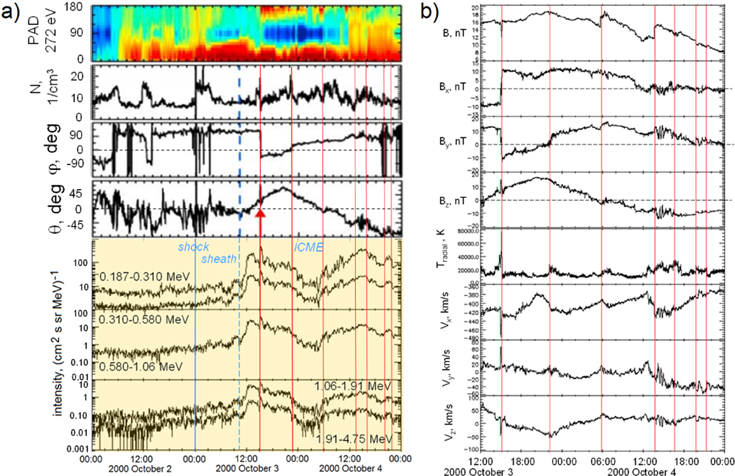
Figure 2. Event 1 AEPE and corresponding plasma/IMF variations associated with an ICME observed on 2000 October 3–4. (a) From top to bottom: suprathermal electron PAD spectrogram, solar wind density, and IMF direction angles; the yellow panel shows the behavior of the energetic ion flux in five energy channels observed by LEMS30. Red vertical lines indicate the positions of SCSs separating flux ropes within the ICME. An arrow identifies the position of an SCS with signatures of Petschek-type magnetic reconnection identified by Gosling et al. (2005). Key IMF/plasma ICME structures are indicated in blue. (b) From top to bottom: IMF components, proton temperature, and three components of the solar wind speed in the GSE coordinate system. The SCSs with signatures of magnetic reconnection are shown by red lines.
Download figure:
Standard image High-resolution imageIt is easy to see that the current sheet selected by Gosling et al. (2005) is not the only reconnecting SCS observed within the ICME. Similar signatures can be found with the crossings of at least six SCSs, as indicated in Figure 2(b) by red vertical lines. The current sheet positions can be identified with crossings of zero in at least one of the three IMF components. Each SCS crossing is associated with increases in the solar wind temperature and at least one of the speed components.
Khabarova & Zank (2017) claimed that DSA at the ICME-driven shock cannot be the source of the AEPE, as the energetic ion time-intensity profiles show only a very minor increase in the lowest energy channels. They showed that (i) particle acceleration was local, as the corresponding peaks in the energetic ion flux time-intensity profiles were also observed by the Wind spacecraft with a time delay corresponding to the solar wind propagation time; (ii) particle acceleration was associated with the crossing of twisted flux ropes or magnetic islands and reconnecting current sheets within the ICME; and (iii) a possible scenario suggested that the mechanism proposed by Zank et al. (2014) might be applied to magnetic islands or highly twisted flux ropes to trap and accelerate energetic ions that were either preaccelerated at reconnecting current sheets or SEP seed particles.
2.2. Second Event: AEPE within an ICME Observed on 1998 October 18–20
This event was first studied by Gosling & Phan (2013) as a part of the investigation of the strong Petschek-like reconnection exhaust observed within an ICME that passed the Earth on 1998 October 18–20, although energetic particle observations were not shown. Khabarova & Zank (2017) discussed the 1998 October 19–20 AEPE that occured within the ICME to illustrate how different particle acceleration mechanisms form energetic ion flux time-intensity profiles associated with the propagation of an ICME. Figure 3(a) is adapted from Figure 12 of Khabarova & Zank (2017). It shows how energetic ion flux profiles change with increasing energy. Time-intersity profiles of the energetic ion flux in low energy channels are characterized by increases at the shock position, suggesting the possibility of DSA, but the energetic ion flux in high-energy channels reveals a dominating increase within the ICME, analogous to the previous event. Figure 3(b) is similar to Figure 2(b). Current sheets with signatures of magnetic reconnection are indicated by red lines, and the upper panel shows how suprathermal electrons change their direction during the passage of the twisted and fragmented magnetic cloud, forming two stripes of bidirectional strahls in the PAD.

Figure 3. Event 2 AEPE and corresponding plasma/IMF variations associated with the ICME observed on 1998 October 19–20. (a) From top to bottom: IMF intensity, solar wind density, solar wind speed, and energetic ion flux observations in three energy channels from two differently directed twin telescopes. The blue line is the ICME-driven shock, and the red line is the reconnection exhaust separating the ICME sheath from the main body of the ICME detected by Gosling & Phan (2013). (b) From top to bottom: electron PAD in the 272 eV energy channel and IMF and plasma parameters analogous to Figure 2(b).
Download figure:
Standard image High-resolution imageSignatures of magnetic reconnection are a little clearer here than in the previous event, especially in the solar wind speed. However, it should be understood that the ACE Solar Wind Electron, Proton, and Alpha Monitor (SWEPAM) time resolution for plasma is 64 s, compared to 1 s resolution for the IMF, which is often insufficient for obvious detection of short-term spikes in the speed, density, and temperature. As a result, the profiles display more gradual peaks around the reconnecting current sheet position.
As one can see from Figure 3, this event is very similar to event 1. Particles are predominantly accelerated inside a twisted ICME, and the DSA mechanism seems to be far less effective.
2.3. Third Event: HCS–CIR Interaction Case. AEPE Associated with the HCS Crossing Observed on 1998 December 24–25
The relationship between CIRs and the HCS is well known (Odstrcil 2003). It was noticed at the beginning of the space era that the HCS either precedes or follows CIRs. It is obvious from Figure 1 that, depending on position, a spacecraft can cross the HCS almost simultaneously with the crossing of the stream interface (SI) of a CIR or with a significant time delay. Both scenarios are often observed in the inner heliosphere. Several episodes of the CIR–HCS interaction and formation of magnetic cavities in front of CIRs were analyzed in our earlier studies (Khabarova et al. 2016, 2018a). In all events, the atypical energetic particle flux enhancements observed before the crossing of the CIR leading edge were associated with the HPS crossing. The HPS in which the HCS is embedded is often thought to represent a simple extension of the streamer belt (Crooker et al. 1993; Liu et al. 2014; Kislov et al. 2015). However, recent observations and theoretical models show that the HPS has a rather complex origin, since plasma signatures of streamers disappear much closer to the Sun than 1 au; therefore, local processes such as magnetic reconnection at the HCS may play an important role, forming a wide HPS, the area around which is filled with magnetic reconnection–related structures (Lepping et al. 1996).
In this study, we analyze a crossing of the reconnecting HCS identified by Gosling et al. (2006). The event was identified as special in terms of the observation of closed magnetic field lines near the HCS. Gosling et al. (2006) selected an SCS with obvious signatures of magnetic reconnection and found that its crossing was characterized by sharp changes in the IMF direction and PADs typical of the HCS. Although Gosling et al. (2006) noticed that the crossing was observed in the vicinity of a high-speed solar wind stream, no obvious connection was suggested. Energetic particle flux profiles were not analyzed in Gosling et al. (2006) either.
Figure 4 shows the behavior of the solar wind plasma and IMF parameters over a little wider time interval than analyzed by Gosling et al. (2006). The CIR region is indicated by the green shading, the HPS area is shown in purple, and the SMI region near the HPS is marked by the yellow shaded region in both Figures 4(a) and (b). In Figure 4(a), along with the plasma parameters, we show the energetic ion (mainly proton) flux time-intensity profiles in selected channels of the LEMS30 EPAM telescope, and Figure 4(b) shows LEMS120 data in one energy channel for comparison. One can find that the behavior of the energetic ion flux detected by both EPAM telescopes is very similar. This is one of the specific properties of particle acceleration associated with SMIs. Since the acceleration process is stochastic, and the flux of energized ions is formed in many places in the region, the anisotropy in such events is usually much weaker than in the case of energetic particles coming from a distant source, i.e., from the Sun or CIR-associated shocks formed at 2–3 au. As a result, Sun-facing LEMS30 and Earth-facing LEMS120 show practically the same averaged time-intensity profiles of the energetic ion flux. In this study, we prefer using LEMS30 for our aims, as LEMS120 data in low- and middle-energy channels are often contaminated by numerous sharp spikes formed by ions reflected from and reaccelerated at the terrestrial bow shock, which complicates the analysis considerably. A comprehensive description of the properties of the LEMS telescopes, as well as the so-called "magnetospheric ions" issue, can be found in Khabarova & Zank (2017).

Figure 4. Event 3 plasma, IMF, and energetic particle flux parameters characterizing an HPS–CIR interaction and the corresponding local particle acceleration observed on 1998 December 24–25. (a) From top to bottom: plasma β, solar wind density, solar wind speed, IMF strength, and LEMS30 ACE EPAM measurements of the energetic ion flux in selected energy channels for the full period of observations of the HPS and CIR, 1998 December 24–27. (b) Selected parameters for a shorter period encompassing the HCS crossing and the energetic particle flux enhancement associated with SMIs. From top to bottom: electron PADs for suprathermal electrons of 1370 and 272 eV energies, plasma β, clock angle of the IMF, two horizontal components of the IMF (GSE coordinate system), and energetic ion flux measurements in the 1.91–4.75 MeV energy channel from the two EPAM telescopes: LEMS30 and LEMS120.
Download figure:
Standard image High-resolution imageThe strongest current sheets observed during the period of interest are indicated by the red vertical dashed lines in Figure 4(a). The SCSs can be identified by simultaneous jumps of the plasma β and drops in the IMF strength as at least one of the IMF components becomes zero, and an SCS is always characterized by an increased plasma density. The crossing of an SCS, considered by Gosling et al. (2006) as the HCS, occurred on 1998 December 25 at 5:36 UT (red vertical solid line in Figure 4(a)). However, it is obvious that a high-plasma-β region with several peaks that almost reached or even exceeded 100 was observed several hours before the reconnecting SCS identified by Gosling et al. (2006). The latter was the last of a row of SCSs with a plasma β above 1.
Suprathermal electrons with an energy of 272 eV are very sensitive to local magnetic structures. They can be produced not only in the corona but also by magnetic reconnection at SCSs directly in the solar wind (Zharkova & Khabarova 2012; Egedal et al. 2015). It has been shown that the observation of bidirectional (counterstreaming) strahls, identified by the two horizontal stripes in the 272 eV PAD, is typical for crossings of an SMI-associated region (Khabarova et al. 2016, 2018a; Khabarova & Zank 2017). At the same time, suprathermal electrons with a much higher energy (1370 eV) undoubtedly originate in the corona and almost do not respond to local magnetic structures. The corresponding 1370 eV PAD in Figure 4(b) shows the sharp change of the strahl propagation direction, which is characteristic for an IMF polarity change, several hours before the crossing of the reconnecting SCS analyzed by Gosling et al. (2006). The HCS was crossed at the HPS left edge, and the IMF direction became stable until the crossing of the SI of the CIR.
This particular CIR had a quite typical profile. It was preceded by a gradual increase of the solar wind density that started from the beginning of December 24 and was followed by a density decrease, while the solar wind speed began to increase at the beginning of December 25. The CIR can be found in the list of CIRs and transient SIRs compiled by Lan Jian: http://www-ssc.igpp.ucla.edu/~jlan/ACE/Level3/SIR_List_from_Lan_Jian.pdf. Lan Jian suggested from an analysis of plasma parameters that the leading edge of the CIR, the SI, was observed at 2:00 UT on 1998 December 25. The detailed analysis of PADs and the IMF direction in Figure 4(b) allows us to correct this conclusion, and we suggest that the SI was crossed at 5:36 UT, bringing an SCS at its front. Indeed, besides the steplike increase in the solar wind speed that occurred simultaneously with the decrease in the solar wind density (Figure 4(a)), the suprathermal electron PAD in the 272 eV channel shows a characteristic vertical stripe (Rouillard et al. 2010), after which the behavior of the IMF components becomes far more turbulent (Figure 4(b)). The CIR brings a change in the IMF direction illustrated by the sharp variation in the IMF clock angle and the PADs in the 1370 and 272 eV channels.
The analysis of electron PAD spectrograms combined with the classical identification of SCSs and the HPS by IMF changes allows us to conclude that the ACE spacecraft entered the high-β area of the unstable IMF direction characterized by short excursions in the IMF direction and rotating magnetic field first (yellow SMI region in Figure 4(a)), and then the HPS was crossed (purple region). The α particle–versus–proton ratio was low during the entire period shown in Figure 4, but it had a minimum below 0.01 in the HPS area (not shown). As mentioned above, the HPS also contains SMIs and small-scale current sheets, although the SMIs observed here are usually smaller and more irregular in comparison with the region outside the HPS. Figure 5(a) illustrates this, showing the IMF rotation in the ecliptic plane that can be easily observed with 4 minute IMF data within the SMI region, while the presence of the closed IMF line within the HPS and near the HCS can be revealed with higher-resolution data, as shown by Gosling et al. (2006).
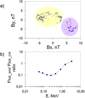
Figure 5. (a) IMF hodogram plotted for the in-ecliptic IMF components for the SMI (yellow) and HPS (purple) periods and (b) the dynamics of the relative intensity of the energetic ion flux associated with SMIs (Flux_smi) and CIR (Flux_CIR). The ratio is calculated for the corresponding maxima of Flux_smi and Flux_CIR observed by LEMS30 in all energy channels. Panel (a) shows the rotation of the IMF vector in the XY direction within the SMI region, while SMIs in the HPS region are far more irregular and smaller. As a result, the rotation in the latter region is seen only at higher resolution, as shown in Gosling et al. (2006). Panel (b) is an illustration of the competition between "classic" CIR-associated particle acceleration and particle acceleration associated with SMIs, as predicted by Zank et al. (2014, 2015).
Download figure:
Standard image High-resolution imageAccording to Figure 4, the energetic ion flux observed in different energy channels behaved typically for local particle acceleration by dynamical SMIs (Khabarova & Zank 2017). Seed particles were initially energized by magnetic reconnection at the SCS identified by Gosling et al. (2006) and other reconnecting SCSs in the SMI and HPS regions. A small local peak is seen around the SCS position (red line in Figure 4(a)) in the lower-energy channel to the left of the classical energetic ion flux enhancement associated with the CIR (green shaded region). In the middle-energy range, the local peak near the main reconnecting SCS is not so obvious, but at the same time, the energetic ion flux enhancements are observed in the HPS area (purple region) and the area filled with SMIs (yellow region). Notice that the ion flux enhancements are in the vicinity of the HCS. The energetic electron flux looks approximately like the energetic ion flux in the lower panels of Figure 2(b) (not shown).
The coexistence of different mechanisms of particle acceleration operating in the same plasma and IMF conditions and configurations has been illustrated in Khabarova & Zank (2017) for the ICME case (events 1 and 2, this manuscript). Generally, the entire picture of the dominance of one mechanism over another in different energy ranges resembles that shown in Figure 4(a). We have done a simple analysis to show the dynamics of the interplay between two mechanisms of particle acceleration that form the observed energetic ion flux time-intensity profiles shown in Figure 4. If one suggests that the energetic flux enhancement observed within the CIR (green) region in Figure 4 is mostly associated with DSA occurring at CIR-associated shocks, and the energetic ion flux enhancement in the yellow and purple HCS-associated regions is determined by SMI dynamics, then it is easy to find at which energies one mechanism dominates the other. One can calculate the ratio of maximal intensity obtained by energetic ions in different energy channels within the HPS/SMI (purple and yellow) regions versus the CIR (green) region. Figure 5(b) shows a steady increase in the ratio, which illustrates the fact that the particle acceleration mechanism determined by processes in dynamical SMIs (Zank et al. 2014, 2015; le Roux et al. 2015, 2016, 2018) becomes more important at higher energies compared to classical DSA occurring at the CIR-related shocks.
After performing a detailed analysis of the CIR–HCS interaction, we can reconstruct the chain of events that occurred on 1998 December 24–25. Figure 6(a) reproduces the interpretation of the event given by Gosling et al. (2006). It was suggested that the HCS experienced magnetic reconnection, and, as a result, ACE detected a single loop of the reconnection exhaust rooted in the corona. Counterstreaming electrons were believed to be produced in the corona only, and no other sources of bidirectional strahls were suggested.
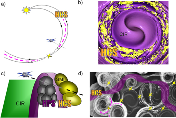
Figure 6. Cartoon showing the formation of closed IMF structures and the interpretation of observations of bidirectional (counterstreaming) strahls near the HCS from different perspectives. (a) Sketch showing the formation of a closed IMF loop via a single Petschek-like magnetic reconnection event at the HCS (dashed purple line). The IMF field lines are directed differently on the two sides of the HCS. It is possible that a spacecraft can eventually cross the closed IMF lines connected to the Sun. This panel is adapted from Gosling et al. (2006). (b) Cartoon showing the formation of magnetic cavities between a rotating CIR and the HCS. The magnetic cavities are filled with the products of magnetic reconnection, including waves and magnetic islands (indicated with yellow). (c) Illustration of the HCS–HPS–CIR crossing observed on 1998 December 24–25. The purple region is the HCS surrounded by SMIs in front of the approaching CIR (green region). Formally, both the yellow and gray areas are a part of the rippled HPS. However, to distinguish between the SMIs trapped inside the formed magnetic cavity and the SMIs that can still be advected by the solar wind, we call only the part inside the ripple "HPS." (d) Rotation of the local magnetic field in SMIs observed near the HCS (purple stripe). Stochastic magnetic reconnection occurs at small-scale current sheets separating SMIs of the same chirality (the reconnection sites are shown by diamonds). Purple arrows show the direction of propagation of suprathermal electrons produced by magnetic reconnection. As a result, counterstreaming strahls are observed in PADs.
Download figure:
Standard image High-resolution imageIt should be noted that Gosling et al. (2006) correctly suggested the presence of the closed magnetic field lines, but the interpretation is too simplified to explain all of the observed changes in the solar wind parameters. Furthermore, such small-scale loops cannot survive in the solar wind owing to numerous instabilities, as a result of which a loop of the size suggested by Gosling et al. (2006) would pinch and be detached from the Sun, forming an elongated SMI. Indeed, the smaller the scale of a structure, the more likely it was produced relatively nearby.
The cartoons we plot in Figures 6(b) and (c) to interpret the observed IMF/plasma changes effectively show Figure 4(a) in 3D. The magnetic cavity formed between the CIR and the HCS is filled with waves, SMIs, discontinuities, and current sheets (shown in yellow in Figure 6(b), see also a similar sketch in Khabarova et al. 2018b). The 3D picture offers numerous scenarios for the HCS–CIR pair crossing, including that shown in Figure 6(c), which corresponds to the examined case best of all. The scenario is similar to that of the double crossing of the HCS presented in Figure 1. First, ACE enters a region filled with SMIs near the HCS. The SMIs in front of the HCS are marked in yellow in Figure 6(c) for the reader's convenience so that they can correlate it with Figure 4(a). However, the SMIs can be treated generally as a part of the HPS from the other side of the rippled HCS. The IMF direction becomes unstable in this region, and counterstreaming strahls and dropouts are observed. Then the HCS is crossed, the IMF direction changes, and the ACE spacecraft finds itself within the internal HPS region for several hours. In this case, the HPS region ends with the SI crossing. Finally, ACE enters the CIR that carries the same IMF direction as in the beginning of the event.
Generally, in the planar undisturbed case, the HCS is embedded in the HPS and located somewhere in the middle of it (Simunac et al. 2012). However, it was recognized many years ago that the HCS is sometimes located at the very edge of the HPS (Liu et al. 2014). Recent results suggest that this is often a signature of the distortion of the HPS and the formation of ripples. As noted above, the HPS region is also filled with SMIs. However, the biggest SMIs are observed not in the HPS but rather in its vicinity. Besides the initial magnetic reconnection that takes place at the HCS and produces SMIs, stochastic or turbulent magnetic reconnection occurs in numerous regions around the HCS at small-scale current sheets separating SMIs, as illustrated in Figure 6(d). The reconnection sites are shown by yellow diamonds in Figure 6(d). As a result, before the HPS crossing, a spacecraft usually observes an SMI region where counterstreaming strahls are produced by the local magnetic reconnection. The direction of propagation of counterstreaming strahls for a pair of merging and reconnecting SMIs is shown by purple arrows in the bottom left corner of Figure 6(d). In the general CIR–HCS interaction case, the SMI region may or may not be observed from both sides of the HPS, depending on the position of the spacecraft with regard to the propagating CIR front. During the 1998 December 24–25 event, the SI coincided with the second HCS crossing, as illustrated in Figure 6(c).
3. Theory and Predictions
Charged particles that propagate in a "sea" of magnetic islands experience several forces that are generated by the dynamical evolving magnetic islands. Charged particles encounter multiple magnetic islands and respond individually and collectively to the islands' dynamics. During these interactions, charged particles can gain energy. Three fundamental mechanisms are understood to energize charged particles via magnetic islands. The first process is associated with island contraction and yields a first-order Fermi acceleration mechanism (Drake et al. 2006). In the second process, a second-order Fermi acceleration mechanism is related to particle acceleration due to the random motion of the magnetic island. If the magnetic islands oscillate or bounce, the trapped particles may undergo second-order Fermi energization. Due to the shortening of the magnetic field line of the magnetic island during the merging of two adjacent islands, the particles can also obtain energy through second-order Fermi acceleration. In the merging process, the shortening of magnetic field lines results in an increase in the velocity component parallel to the local magnetic field and a decrease in the perpendicular energy (Drake et al. 2013). In the third energization process, the particles trapped in the merged magnetic islands interact with the reconnection electric field induced by the merging of two magnetic islands. The interaction time between the captured particles and the reconnection electric field is prolonged, resulting in a significant energy gain (Oka et al. 2010). Zank et al. (2014) included all possible reconnection-related processes in a dissipative multireconnection supersonic solar wind and formulated a transport equation for a gyrotropic distribution of particles experiencing pitch-angle scattering and energization. The gyrophase-averaged transport equation of Zank et al. describes the transport of charged particles in a region of characteristic size L that is much larger than the characteristic size of magnetic islands l, i.e., L ≫ l. The gyrophase-averaged transport equation is (Zank et al. 2014)
where the simplest form of isotropic (in pitch angle θ, μ ≡ cos θ) scattering operator is assumed,
and νs = 1/τs and  is a characteristic pitch-angle scattering time, and Ω = eB/m is the particle gyrofrequency. The parameters ηc and ηm are characteristic magnetic island contraction and merging rates, μ denotes the cosine of the particle pitch angle,
  is the direction of the local magnetic field, v is the particle speed, U is the bulk flow velocity, and δE3 is the ensemble-averaged antireconnection electric field parallel to the magnetic field. In Equation (1), the terms proportional to ∝v∂f/∂v describe the particle acceleration processes, in which one term includes the divergence of the large-scale bulk flow and the other term contains the small-scale effect of island contraction and merging.
Zank et al. simplified Equation (1) by assuming a nearly isotropic particle distribution and derived a transport equation in the phase-space conservation form (Zank et al. 2014)
where
is the energetic particle streaming in space,
is the streaming in momentum space, and the diffusion coefficient in velocity space is given by
Zank et al. (2014) further considered an incompressible super-Alfvénic flow,  , with a steady injection of particles of fixed initial speed v0 at the origin and restricted the analysis to 1D. They also assumed for analytic convenience that the spatial diffusion coefficient is constant and neglected the second-order energy diffusion terms. However, Zank et al. did not consider particle escape from an enclosed region of multiscale magnetic islands. It is likely that particles will escape from a spatially limited region. Zhao et al. (2018) considered particle escape and accordingly modified the steady-state transport equation of Zank et al. by including the escape term as
where  ,
,  is the logarithm of the ratio of the particle speed,
  is a scattered antireconnection electric field–induced velocity,
  is the fluctuating reconnection electric field, and τesc is the particle escape time. The parameter n0 is the particle number density, v0 is the initial speed at the origin, and k is the spatial diffusion coefficient. The general solution of Equation (3) can be obtained as (Zank et al. 2014; Zhao et al. 2018)
where ME = U/VE, I0 is the modified Bessel function of order 0, and H[...] is the Heaviside function. The parameter τdiff ≡ k/U2 is the diffusive timescale, τc = η−1 is the magnetic island contraction timescale, and Ldiff ≡ k/U is the diffusion length scale. The general solution, Equation (4), combines the effects of both the reconnection-induced electric field due to island merging and plasmoid contraction. Equation (4) also indicates that the accelerated particles form a power law in particle speed with an index depending on τdiff/τc, τdiff/τesc, and ME. Moreover, Equation (4) also exhibits an "amplification factor" property, as described by Figure 7. Figure 7 is a sketch of the normalized solution of Equation (4) at the injection position (IP) x0, in which the normalized distribution function  is larger than 1 downstream of x0 and exhibits an exponential decay upstream of x0. A flux amplification larger than 1 indicates stochastic energization of charged particles in a region filled with numerous SMIs. Similarly, exponential decay of the normalized distribution function is associated with diffusion of particles into the upstream flow. The power-law solution of Equation (4) in particle velocity v can be approximated as (Zank et al. 2014; Zhao et al. 2018)
We note that Equations (4) and (5) differ from Equations (39) and (40) of Zank et al. (2014) by the particle escape term  .
.
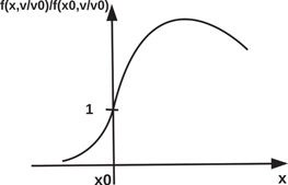
Figure 7. Sketch of Equation (4), illustrating the "amplification factor." The normalized distribution function,  , decays exponentially upstream from the IP x0 and becomes larger than 1 downstream of the IP for the particular values of ME, τdiff/τc, and τdiff/τesc.
Download figure:
Standard image High-resolution imageIt is useful to write Equation (4) in terms of the differential intensity j(E) so that one can directly match the solution to the spacecraft measurements (Zhao et al. 2018),
where

describes the relationship between the distribution function and the differential intensity. The parameter j0 is a normalization constant, and E0 is the energy corresponding to the particle speed v0.
4. Results
In this section, we calculate the observed flux amplification and intensity profiles associated with AEPEs 1, 2, and 3, discussed in Section 2. We compare the observed results with our theoretical solutions. To compare the theoretical and observed results, we first transform the time of measurement of ion flux t into a spatial distance X using the relation X = U (−t + t0), where the solar wind speed U ∼ 400 km s−1 is assumed, and t0 corresponds to the observation time of a reconnecting current sheet. The spatial distance X is then normalized to the diffusion length scale Ldiff, i.e.,  . We calculate the observed and theoretical flux amplifications by normalizing the fluxes at the IP. The IPs, for example, are shown by the vertical red lines in Figures 2–4. In calculating the theoretical differential intensity at various distances, we first find the constant j0 corresponding to the IP using a least-squares method on Equation (6), which yields
where N is the total number of different energy channel ion fluxes at the IP,  , and
, and  . Here ji and Ei denote the energetic ion flux intensity and the particle energy at the IP. Then, we use the value j0 in Equation (6) to obtain the theoretical differential intensities at various distances.
The comparison between the theoretical and observed flux amplifications for the different energy channels of the three events as a function of normalized spatial distance  is shown in Figure 8. Figure 8 provides possible evidence for the local acceleration of energetic particles associated with reconnection exhausts. In the figure, amplification factors are larger than 1 downstream of reconnection exhausts, suggesting the local acceleration of particles via reconnection-associated processes with dynamically evolving and merging magnetic islands. Figure 8 shows that the observed flux amplifications are in accord with the amplification rule predicted by the theoretical curves (see Figure 7, for example). Also, note that the ordering of the amplification factor increases with energy; i.e., the largest amplification factor occurs for the largest energy particles, and vice versa. In Figure 8, the dashed curves are the observed normalized flux amplifications, and the solid curves are the theoretical normalized flux amplifications. Furthermore, the dashed curves, i.e., the observed flux amplifications, show an exponential decay upstream of the reconnecting current sheets that is due to the diffusion of particles against the flow in the upstream region (Zank et al. 2014). The way in which the theoretical solution of Zank et al. (2014) is constructed from the transport equation shows that if particles are injected at a given point in a flowing medium, then the particles are advected and diffused downstream of the particle source but can only diffuse upstream from the source—the solution in the upstream direction will have the form of an exponential decaying solution with a scale length of κ/U.

Figure 8. Comparison between the theoretical and observed flux amplifications of energetic ion flux in different energy channels as a function of normalized spatial distance  . The top, middle, and bottom panels correspond to events 1, 2, and 3, respectively. The solid and dashed curves are the theoretical and observed flux amplifications.
Download figure:
Standard image High-resolution imageThe flux amplification shown in the top panel of Figure 8 is associated with event 1. In the figure, the three humps indicated by the observed results may be a manifestation of individual or collective islands that can trap particles temporarily and lead to local enhancements. Here the SCS position is at 2000 October 3 23:00:00 UT, which is equivalent to  in our theoretical solution. The normalized solution of Equation (4) requires the values of three parameters: the ratio of the particle diffusion timescale to the magnetic island contraction timescale
  , ME, and the ratio of the diffusion timescale to the escape timescale τdiff/τesc. The best-fit parameter values we find are ME = 15, τdiff/τc = 0.1, τdiff/τesc = 3.5, and Ldiff = 2.93 ×10⁵ km. The six solid curves are solutions for different values of the normalized particle speed v/v0, where the magenta curve uses v/
 , the cyan curve v/
 , the green curve v/
 , the black curve v/
 , the blue curve v/
 , and the red curve v/
 . Thus, the energy ranges from
  to
to  ; i.e., the maximum energy is 17 times the minimum energy. Even though the theoretical and observed flux amplifications show similar trends, the solid curves reach peak values earlier than the dashed curves. The observed flux amplification increases slowly with
  , in contrast to the theoretical flux amplification. However, the observed flux amplification at larger distances downstream of the IP is approximately twice that at closer distances from the IP. The variation in the observed flux amplification may be due to changes in the magnetic islands' topology with distance.
The middle panel of Figure 8 corresponds to event 2. In this event, as shown by red vertical lines (see Figure 3(b)), there are many current sheets. Here we choose two reconnecting current sheet positions at 1998 October 19 14:00:00 UT and 1998 October 20 4:00:00 UT, which are equivalent to  and
and  in our theoretical solution. In the middle panel (Figure 8), there is a gap in the flux amplification at
  because the ion flux is normalized at
  for the region
  . We calculate the observed flux amplifications in the regions
  and
and  independently. In the first region, we use ME = 15,
  ,
,  , and
, and  km, and the magenta curve corresponds to v/
 , the blue curve to v/
 , the cyan curve to v/
 , and the red curve to v/
 . Hence, the particle energy varies from
  to
to  , producing a maximum energy ∼5.48 times the minimum energy. The comparison shows that the theoretical and measured results are basically consistent. In the second region, we employ ME = 15, τdiff/τc = 0.3,
  , and Ldiff = 7.62 × 10⁵ km (i.e., a very similar set of parameters), in which the magenta curve corresponds to v/
 , the blue curve to v/v0 =64.42, the cyan curve to v/v0 = 86.31, and the red curve to v/v0 = 117.05. The energy ranges from
  to
to  , giving a maximum energy ∼5.48 times the minimum energy. Here the amplification shown by the solid magenta, blue, and cyan curves is initially larger than that of the corresponding dashed curves in the range
  , after which both results are approximately similar. In contrast, the solid and dashed red curves show similar trends from
  to ∼40, after which the dashed curve is higher than the solid curve.
The bottom panel of Figure 8 displays the flux amplification corresponding to event 3. In this event, the reconnecting current sheet is observed at 1998 December 25 05:00:00 UT (see Figure 4(a)), which is an SI between the HPS and CIR. In our theoretical solution, it is equivalent to  . It shows that the theoretical results are larger than the observed results from
  to
to  , and then both results are approximately similar from
  to
to  . Here we use ME = 17, τdiff/τc = 0.114, τdiff/τesc = 4, and Ldiff = 6.69 × 10⁵ km. The cyan curve uses v/v0 = 4.96, the green curve v/v0 = 6.68, and the blue curve v/v0 = 10. Here the energy varies from
  to
to  ; i.e., the maximum energy is ∼4.06 times the minimum energy. Recall that the reconnection exhausts in the top and middle panels of Figure 8 are driven by the ICMEs, while the reconnection exhaust corresponding to the bottom panel is associated with a crossing of the HCS. It appears that the amplification factors associated with reconnection exhausts, i.e., events 1 and 2, are comparatively larger than the amplification factor corresponding to event 3. It is possible that multiscale magnetic islands in the vicinity of the reconnecting current sheets driven by the ICMEs are more favorable to energize the charged particles than those not driven by the ICMEs. However, more study is needed to fully understand the possible differences in the efficiency of the energization of charged particles associated with reconnection exhausts within the ICMEs versus the HCS. Interestingly, the observed flux amplification in the region
  is larger than the flux amplification in the region
  . We note that the region
  is the HPS, and the region
  is related to the SMIs shown by the yellow region in Figure 4.
In Figure 8, there is a noticeable difference between the theoretical and observed flux amplification up to a certain distance downstream of the IP in events 1 and 3. The difference between the theoretical and observed flux amplification behind/downstream of the injection point may stem from the idealized theoretical model of particle acceleration and the evolution of flux ropes developed in Zank et al. (2014, 2015). Specifically, the model of particle acceleration assumes that the magnetic island turbulence behind a reconnecting current sheet (or shock wave) is already fully developed. However, there is likely to be an advective and/or turbulence timescale ( or
or  , where l may be a characteristic magnetic island scale size) that crudely determines when the turbulent interaction of magnetic islands is fully developed. Prior to the complete dynamical interaction of magnetic flux ropes (island merging, contraction), particle acceleration by these processes will be either limited or inefficient. Thus, we expect efficient particle acceleration to occur a short distance away from the injection point once the islands are fully developed and interacting dynamically. Hence, particles tend to gain energy further downstream than they do near the injection location. Here events 1 and 3 may reflect this behavior, whereas event 2 may reflect conditions conducive (or already existing) for fully developed turbulence near the injection point.
The energetic particles in the vicinity of reconnecting current sheets can also be analyzed through the energetic ion flux intensity spectra. Figure 9 provides a comparison between the observed and theoretical differential intensity of ion flux at  9.83, 19.67, 34.42, 39.33, and 49.17 for event 1. For clarity, these locations are identified in the top panel of Figure 8 so that one can easily observe the consistency between the flux amplification and the intensity spectra. In Figure 9, the scatter plots are the measured particle differential intensities, and the solid lines are the theoretical intensities. We use Equation (6) to calculate the theoretical intensity, for which we use the same parameter values, ME = 15, τdiff/τc = 0.1, and τdiff/τesc =3.5, that were applied for the top panel of Figure 8. We first calculate j0 by using Equation (8) with particle intensities at the injection point
  (cyan circles), which yields j0 = 9.37 ×10¹⁵ (cm2 s sr MeV)−1. Using this value of j0 in Equation (6), we calculate the intensity spectra at
  9.83, 19.67, 34.42, 39.33, and 49.17. We find that the theoretical intensity profile (cyan solid line) of Equation (6) is very similar to that of the observed intensity at
  (cyan circles). However, the theoretical intensities at
  , 19.67, 34.42, and 44.25 are larger than those of the corresponding observed intensities, whereas both the theoretical and observed intensities at
  are the same, and the theoretical intensity at
  is smaller than the observed intensity.

Figure 9. Comparison between the theoretical and observed energetic particle flux intensity spectra at different locations  = 0, 9.83, 19.67, 34.42, 39.33, 44.25, and 49.17 corresponding to event 1. The scatter plots denote the measured energetic particle flux intensity, and the solid lines are the theoretical intensities. Both theoretical and observed particle flux intensities, indicated by magenta, red, blue, black, green, and yellow, are multiplied by 1.2, 2, 3, 4, 8, and 10, respectively, to distinguish one from the other.
Download figure:
Standard image High-resolution imageFigure 10 compares the theoretical and observed differential intensity spectra of event 2. In the figure, the left panel shows the particle flux intensity spectra at  3.78, 7.56, 9.44, 11.33, and 13.22 (see also middle panel of Figure 8). We use the same parameter values, ME = 15,
  , and τdiff/τesc = 6, as used for the middle panel of Figure 8 (
 ). We find j0 = 1.4 × 10⁷ (cm2 s sr MeV)−1. The theoretical (solid cyan curve) and observed (cyan circle) spectra match each other very well at the injection point. Similarly, the theoretical and observed differential intensity spectra at other locations are also almost identical. The spectrum at the IP
  is steep and becomes harder with increasing
  .
.

Figure 10. Comparison between the theoretical and observed energetic ion flux intensity affiliated with reconnection exhausts corresponding to event 2. Left: Spectra at distances  3.78, 7.56, 9.44, 11.33, and 13.22 are shown in the middle panel of Figure 8. Right: Spectra at distances
  30.22, 34, 37.78, 39.67, and 43.44 are shown in the middle panel of Figure 8. Both theoretical and observed results, indicated by red, blue, black, and green, are multiplied by 2, 4, 6, and 10, respectively.
Download figure:
Standard image High-resolution imageThe right panel of Figure 10 describes the intensity profile at  30.22, 34, 37.78, 39.67, and 43.44. Note that
  is the second IP. Again, the parameter values we use for ME, τdiff/τc, and τdiff/τesc are the same as for the middle right panel of Figure 8 (
 ). Now j0 = 2.0 ×10⁸ (cm2 s sr MeV)−1. The comparison shows that the theoretical and observed intensity spectrum at
  is almost identical, and that the theoretical and observed intensity spectra show similar trends with increasing
  . There appears to be no observed flattening of the spectra at low energies.
The comparison of theoretical and observed particle flux intensity corresponding to event 3 is shown in Figure 11. The theoretical and observed particle flux intensities are calculated at  , 6.46, 15.08, 17.23, 19.38, 21.54, and 23.69. For this case, we obtain j0 = 1.18 × 10⁶ (cm2 s sr MeV)−1. The parameter values for ME, τdiff/τc, and τdiff/τesc are the same as those used for the bottom panel of Figure 8. Figure 11 shows that the theoretical spectra are very similar to the measured intensity spectra at
  , 15.08, and 17.23, whereas the theoretical and observed results at other locations are a little different from each other.
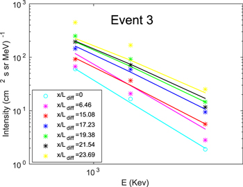
Figure 11. Comparison between the theoretical and observed energetic ion flux at  , 6.46, 15.08, 17.23, 19.38, 21.54, and 23.69 associated with the reconnection exhaust corresponding to event 3. Both theoretical and observed results, indicated by blue, green, black, and yellow, are multiplied by 2, 3, 4, and 6, respectively.
Download figure:
Standard image High-resolution imageThe energetic particle flux intensities shown in Figures 9–11 indicate that the spectra at the IP are steep, and the spectra at larger distances downstream from the IPs are harder. In each event, the theoretical and observed energetic ion flux intensity at the IP is very similar, because the amplitude parameter j0 is calculated by the least-squares method using the values of the energetic ion flux intensity (j) and particle energy (E) corresponding to the IP. Similar to the flux amplification, due to the idealized theoretical model of particle acceleration and the evolution of the flux ropes, the theoretical and observed particle flux intensity in the downstream of the injection point may also differ slightly. We calculate the spectral index of each spectrum associated with Figures 9, 10, and 11, i.e., events 1, 2, and 3, respectively, and show the spectral indices in the top, middle, and bottom panels of Figure 12, respectively. Here red diamonds refer to the theoretical spectral indices, blue stars to the observed spectral indices, and vertical dashed lines to the IP. In the middle panel, IP1 and IP2 identify the two injection points of event 2. Both the theoretical and observed spectral indices show similar trends with distance. The theoretical index shows a linear increase with distance, while the observed spectral indices at larger distances tend to decrease compared to those observed close to the IP, although not always. For example, in the top panel of Figure 12 (event 1), the observed spectral indices at  and
and  are −1.91 and −2.24, respectively. In contrast to events 1 and 2, the observed spectral index in event 3 decreases with increasing
  beyond
  . In our analysis, the theoretical and observed spectral indices vary from ∼−1 to ∼−2.5. Furthermore, it shows that the differential intensity spectra at the IP corresponding to events 1 and 3 are steeper than the differential intensity spectrum related to event 2. In addition, Figure 11 also shows the flattening of the theoretical and observed particle intensities with distance.

Figure 12. Comparison between theoretical and observed spectral indices as a function of normalized spatial distance  . The top, middle, and bottom panels show the spectral indices corresponding to events 1, 2, and 3, respectively. Red diamonds and blue stars denote the theoretical and observed spectral indices. The vertical dashed lines represent the IP. Here IP1 and IP2 are the first and second IPs corresponding to event 2.
Download figure:
Standard image High-resolution image
5. Discussion and Conclusions
We have analyzed unusual or atypical energetic particle events that are not associated with classical mechanisms of particle acceleration like flares or DSA and showed that observed particle energization up to several MeV nuc–1 can be explained by dynamical processes associated with magnetic islands and reconnecting current sheets. The theoretical models developed by Zank et al. (2014) and Zhao et al. (2018) have been employed to compare observations from the ACE spacecraft with theoretical predictions. We found that particle energization in the vicinity of the reconnecting HCS or SCSs of various origins can be due to processes related to the trapping and acceleration of charged particles within SMIs. Based on the ability of the theory to reproduce observations quite satisfactorily, charged particles appear to be accelerated by dynamical processes in SMIs independently of the way in which those SMIs are formed in the solar wind from different sources. Furthermore, reacceleration of energetic particles can also occur, since the mechanism of Zank et al. (2014) can be applied effectively to any previously existing population of energetic particles produced, for example, by magnetic reconnection at SCSs, by shocks, or by flares.
Two of the three events discussed in our paper occur within the body of a primary ICME event, and one event is associated with the HCS crossing. Generally, magnetic reconnection in the solar wind is stochastic and occurs at many points in an aggregate of magnetic islands and current sheets, which makes it complicated to find direct evidence for 3D magnetic reconnection, but it is sometimes possible to find simple signatures of Petschek-like magnetic reconnection at small-scale current sheets. This may serve as a key for observers to find regions experiencing intensive magnetic reconnection. Two processes responsible for local particle acceleration usually interplay or take place simultaneously. These are merging and contraction of magnetic islands. Contraction is found to enhance particle acceleration in the background of preexisting merging that occurs naturally in the solar wind, according to simulations. For example, in this particular study, we showed particle acceleration in a current sheet–magnetic island system near the HCS as it is compressed by an approaching CIR. In the two ICME cases discussed, magnetic islands experienced active merging and additional compression according to observed density increases inside the main ICME body. To compare observations with theoretical solutions, we computed the flux amplification factor and particle flux intensity for the three events. In each event, we found similar trends between theoretical and observed flux amplifications. The results obtained can be summarized as follows.
- (i)Both observed and theoretical flux amplification factors are larger than 1 downstream of the IP, implying that particle acceleration via reconnection-associated processes with dynamically evolving and merging magnetic islands occurs.
- (ii)The observed flux amplification factor profiles obey the amplification rule predicted by the theoretical solution, in which the order of the amplification factor increases with increasing energy; i.e., the largest amplification factor is for larger-energy particles, and the lowest amplification factor is for lower-energy particles.
- (iii)The amplification factor in each event is different, signifying that the properties, energization efficiency, and topology of the magnetic island–containing region may change downstream of the injection point; hence, the efficiency of the particle acceleration process may also vary with distance.
- (iv)The flux amplification factors corresponding to ICME events are apparently larger than those associated with the HCS crossing event. It suggests that multiscale magnetic islands in the vicinity of reconnecting current sheets within a twisted and fragmented magnetic cloud energize charged particles more effectively than those associated with the HCS, probably because of larger sizes. However, this tentative conclusion requires further investigation before we fully understand the role of ICMEs in the reconnection-associated particle acceleration processes.
- (v)Observed energy spectra are steep in all events discussed above, with slopes from −1 to −2.5, consistent with theoretical predictions.
- (vi)The slope increases with increasing distance with regard to the IP, also consistent with theoretical predictions.
As discussed, theoretical predictions for flux amplification and spectra are consistent with observations, suggesting that local particle acceleration determined by dynamical processes associated with magnetic islands has a significant impact on the time-intensity profiles of energetic particle flux at 1 au in some events. This effect cannot be ignored, as it represents a serious, unexpected, and unpredictable hazard for astronauts and equipment on board spacecraft.
We are grateful to the Goddard Space Flight Center for providing the ACE spacecraft data at http://cdaweb.gsfc.nasa.gov/. The list of reconnection exhaust events can be found at http://www.srl.caltech.edu/ACE/ASC/DATA/level3/swepam/ACE_ExhaustList.pdf. Results of the ENLIL modeling are from http://www.helioweather.net/. We acknowledge the partial support of NSF EPSCoR RII-Track-1 cooperative agreement OIA-1655280; NSF-DOE award 1707247; and NASA grants NNX08AJ33G, subaward 37102-2, NNX14AC08G, NNX14AJ53G, A99132BT, RR185-447/4944336, and NNX 12AB30G. G.P.Z. is partly supported by the International Space Science Institute (ISSI), both through the award of the 2017 Johannes Geiss Fellowship and in the framework of International Team Project 405, titled "Current Sheets, Turbulence, Structures and Particle Acceleration in the Heliosphere." O.V.K. was supported by RFBR grant Nos. 17-02-01328, 17-02-00300, 18-52-06002, and 19-02-00957.