Accurate Laboratory Measurement of the Complete Fine Structure of the N = 1 − 0 Transition of ¹⁵NH

Studies of the nitrogen chemistry in interstellar sources and in solar system bodies carried out over the last two decades have revealed a puzzling isotopic pattern. The measured ${}^{14}{\rm{N}}{/}^{15}{\rm{N}}$ ratio shows an outstanding variability, depending on the sample, type of material, and molecular carrier (see, e.g., Hily-Blant et al. 2013; Füri & Marty 2015, and references therein). Compared to the proto-solar value of ∼440 (measured in the solar wind; Marty et al. 2011) almost all solar system objects are enriched in the heavier isotope: ${}^{14}{\rm{N}}{/}^{15}{\rm{N}}$ is 272 on the Earth (Marty 2012), is ≈150 in comets (Jehin et al. 2009; Bockelée-Morvan et al. 2015; Shinnaka et al. 2016), and is as low as 50–70 in some meteoritic samples (Bonal et al. 2010). These findings clearly suggest the existence of an ${}^{15}{\rm{N}}$-enriched molecular reservoir, yet the question of where and how the isotopic excess is produced has still not received a satisfactory answer.

A gas-phase mechanism based on ion–neutral isotope exchange reactions in the cold interstellar medium was proposed by Terzieva & Herbst (2000) and was subsequently updated by several theoretical studies (e.g., Charnley & Rodgers 2002; Rodgers & Charnley 2008; Wirström et al. 2012). This picture remained fashionable until recently, when a major revision of the nitrogen chemistry network was advocated by Roueff et al. (2015) on the basis of quantum chemical calculations. In this newly proposed scheme, some key isotope exchange processes are suppressed, thus making N fractionation basically ineffective. The present status of the theory has been reviewed recently by Wirström & Charnley (2018). Here we should note that, in its present form, the model is not easily reconcilable with the observations toward cold cloud cores and massive star-forming regions, which found a sizable spread in the ${}^{14}{\rm{N}}{/}^{15}{\rm{N}}$, ranging from clear evidence of fractionation (Daniel et al. 2013) to remarkable cases of depletion (also known as "anti-fractionation," e.g., ∼800–1000 in N₂H⁺; Bizzocchi et al. 2013; Fontani et al. 2015; Redaelli et al. 2018). Insights into possible alternative fractionation pathways may come from future observations targeting all of the relevant molecules, particularly those belonging to the nitrogen hydride family that show the most variable and puzzling isotopic composition. These species ("amines;" see, e.g., Hily-Blant et al. 2013) are generated from N₂ in a chain of reactions starting from the dissociative ionization product, N⁺, e.g.,

$$\begin{eqnarray*}&&{{\rm{N}}}^{+}+{{\rm{H}}}_{2}\to {\mathrm{NH}}^{+}+{\rm{H}},\\ &&{\mathrm{NH}}^{+}+{{\rm{H}}}_{2}\to {\mathrm{NH}}_{2}^{+}+{\rm{H}},\\ &&\ldots .\end{eqnarray*}$$

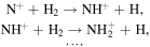
The radical species NH (imidogen) is generated by the electronic recombination of the NH⁺ ion and is thus the simplest neutral species that inherits the isotopic composition of the N₂ reservoir.

Imidogen has been known as a constituent of late-type star atmospheres for a very long time (Shaw 1936; Schmitt 1969). In the early 1990s, the parent NH isotopologue was also detected in the Sun (Geller et al. 1991), in the P/Halley comet (Feldman et al. 1993), and in the diffuse interstellar gas (Meyer & Roth 1991) through high-resolution observations in the infrared and ultraviolet bands. More recently, when Herschel/Heterodyne Instrument for the Far Infrared (HIFI) opened up the far-infrared (FIR) spectral window, the fundamental N = 1 − 0 transition of NH around 1 THz was observed in absorption toward a massive interstellar cloud and in the IRAS 16293-2422 proto-stellar envelope (Hily-Blant et al. 2010; Persson et al. 2010). The deuterated isotopologue ND was also identified in this latter source (Bacmann et al. 2010) and in the prestellar core 16293E (Bacmann et al. 2016), while no detection has been ever reported for the ${}^{15}{\rm{N}}$-containing variant.

Nowadays, after the end of the Herschel mission, THz observations are limited to what is achievable from Earth-based observatories (mainly with the Atacama Large Millimetter/submillimeter Array (ALMA)) or balloon/airborne instruments. In particular, the Stratospheric Observatory for Infrared Astronomy (SOFIA) is a stratospheric facility operating at 41,000 ft (∼12,500 m) that can take advantage of several good transparency windows with transmittance ranging in the 0.4–0.9 interval.⁴ This telescope is being equipped with the new 4-color German REceiver for Astronomy at Terahertz frequencies (4GREAT) heterodyne receiver, which covers all of the four former HIFI bands, thus offering the possibility of observing the same spectral range exploited by Herschel. Still, the detection of the intrinsically weak ${}^{15}\mathrm{NH}$ spectral features constitutes a challenging observational task. Its N = 1 − 0, J = 0–1 fine-structure line falls at the edge of the ALMA band 10, thus requiring long integrations. Also, extreme precision in the rest frequencies is needed to maximize the chance of success.

The spectroscopy of the parent ¹⁴NH isotopologue has been the subject of extensive laboratory investigations (see, e.g., Ram et al. 1999; Flores-Mijangos et al. 2004; Lewen et al. 2004; Robinson et al. 2007 and references therein). On the contrary, the rotational spectrum of ${}^{15}\mathrm{NH}$ has remained unknown until recently. Bailleux et al. (2012) recorded its FIR spectrum at the SOLEIL synchrotron in the 65–225 ${\mathrm{cm}}^{-1}$ range, measuring a sequence of fine-structure triplets up to the rotational $N=7\leftarrow 6$ transition. That study was complemented with the recording of the lower fine-structure component of the fundamental $N=1\leftarrow 0$ line at 942 GHz using a submillimeter spectrometer. Bailluex et al. (2012) then provided predicted rest frequencies for the two fine-structure components (including the strongest, $J=2\leftarrow 1$), which could not be observed because they fell outside the spectral coverage of the spectrometer. It should be noted that THz measurements performed with harmonic multiplication of a synthesized radiation sources are at least a factor of 100 more precise than those obtained with a Fourier-transform infrared spectrometer. Hence, a direct measurement of all of the J components of the $N=1\leftarrow 0$ line is desirable if one aims to use these data to guide sensitive astronomical observations.

In this paper, we present the complete high-resolution laboratory study of the $N=1\leftarrow 0$ rotational transition of ${}^{15}\mathrm{NH}$. The F₁, F multiplets for all of the three J components have been recorded with a fairly high signal-to-noise ratio (S/N) and the corresponding line positions have been accurately determined by means of a line profile analysis. A least-squares fit of both the present work's and literature's (Bailleux et al. 2012) data yielded much improved spectroscopic constants for the ground state and for the newly determined parameters for the v = 1 vibrationally excited state, whose spectral features have been detected for the first time.

The rotational spectrum of ${}^{15}\mathrm{NH}$ was observed in absorption using the Center for Astrochemical Studies Absorption Cell spectrometer at the Max-Planck-Institut für extraterrestrische Physik. The experimental apparatus is described in detail elsewhere (Bizzocchi et al. 2017). Briefly, the instrument employs an active multiplier chain (Virginia Diodes, Inc.) as a source of millimeter radiation in the 82–125 GHz interval. Using two additional frequency tripler stages in cascade, this setup provides operation in the THz regime with an available power of a few μW. A cryogenic-free, closed-cycle cooled InSb hot electron bolometer (QMC Instr. Ltd.) is used as a detector. The absorption cell is a Pyrex tube (3 m long and 5 cm in diameter) containing two stainless steel, cylindrically hollow electrodes separated by 2 m. The plasma region is cooled by liquid nitrogen circulation. The spectrometer employs the frequency modulation (FM) technique to enhance the S/N of the recorded signals. The carrier frequency was sine-wave modulated at a rate of 33.3 kHz, then phase sensitive detection at $2f$ is performed using a digital lock-in amplifier. In this way, the second derivative of the actual absorption profile is recorded by the computer-controlled acquisition system.

The ${}^{15}\mathrm{NH}$ radical was produced in the positive column of a direct current (DC) glow discharge by flowing a mixture of 3 mTorr (0.4 Pa) of ¹⁵N₂, 3 mTorr of H₂, and 25 mTorr (3.3 Pa) of Ar. The cell was cooled at 90–100 K by liquid nitrogen circulation. The optimal conditions, expressing a balance between the signal strength and the discharge generated noise, were obtained by setting a current of 70 mA and an applied voltage of 1.1 kV.

Imidogen is a diatomic radical with two unpaired electrons in its valence shell. The ground electronic state is labeled as ${}^{3}{{\rm{\Sigma }}}^{+}$, i.e., it is characterized by zero orbital angular momentum, L = 0, and electron spin angular momentum of S = 1. This spin interacts with the rotational angular momentum, producing the splitting of the rotational levels into fine-structure triplets. Further couplings originate from the nuclear spins, ${}^{15}{\rm{N}}$ and ${}^{1}{\rm{H}}$ (both with $I=\tfrac{1}{2}$), which interact with the electron spin and molecular rotation to give the full hyperfine structure. Due to the lack of electronic orbital angular momentum, this vector coupling is best described using Hund's case (b) scheme:

$$\begin{eqnarray}&&{\boldsymbol{N}}+{\boldsymbol{S}}={\boldsymbol{J}},\quad {\boldsymbol{J}}+{{\boldsymbol{I}}}_{{\rm{N}}}={{\boldsymbol{F}}}_{1},\\ &&{{\boldsymbol{F}}}_{1}+{{\boldsymbol{I}}}_{{\rm{H}}}={\boldsymbol{F}}.\end{eqnarray} \tag{ 1 }$$

The quantum number N labels the pure rotational energy levels, each of which is split into three broadly separated fine-structure J components: $J=N+1,N,N-1$. For N = 0, only one component (J = 1) exists. The total angular momentum quantum number F is used to label the hyperfine levels and is inclusive of the ${}^{15}{\rm{N}}$ and ${}^{1}{\rm{H}}$ spin–spin and spin–rotation contributions.

The form of the effective Hamiltonian used for the spectral analysis is

$$\begin{eqnarray}&&\hat{H}={\hat{H}}_{\mathrm{rot}}+{\hat{H}}_{\mathrm{fs}}+{\hat{H}}_{\mathrm{hfs}},\end{eqnarray} \tag{ 2 }$$

where ${\hat{H}}_{\mathrm{rot}}$, ${\hat{H}}_{\mathrm{fs}}$, and ${\hat{H}}_{\mathrm{hfs}}$ are the rotational, fine- and hyperfine-structure Hamiltonians, respectively.

The pure rotational term, ${\hat{H}}_{\mathrm{rot}}$, is expressed as N² expansion using the rotational constant, B, and the centrifugal distortion coefficients, D and H:

$$\begin{eqnarray}&&{\hat{H}}_{\mathrm{rot}}=B{{\boldsymbol{N}}}^{2}-D{{\boldsymbol{N}}}^{4}+H{{\boldsymbol{N}}}^{6}.\end{eqnarray} \tag{ 3 }$$

The fine- and hyperfine-structure Hamiltonians can be conveniently expressed by employing the spherical tensor formalism (Brown & Carrington 2003):

$$\begin{eqnarray}&&{\hat{H}}_{\mathrm{fs}}=\displaystyle \frac{2\sqrt{6}}{3}\,\lambda {T}_{q=0}^{2}({\boldsymbol{S}},{\boldsymbol{S}})+(\gamma +{\gamma }_{N}\,{{\boldsymbol{N}}}^{2}){T}^{1}({\boldsymbol{N}})\cdot {T}^{1}({\boldsymbol{S}}),\end{eqnarray} \tag{ 4 }$$

$$\begin{eqnarray}{\hat{H}}_{\mathrm{hfs}} & = & \displaystyle \sum _{i}{b}_{{\rm{F}}}(i){T}^{1}({{\boldsymbol{I}}}_{i})\cdot {T}^{1}({\boldsymbol{S}})+\displaystyle \sum _{i}\displaystyle \frac{\sqrt{6}}{3}c(i){T}_{q=0}^{2}({{\boldsymbol{I}}}_{i},{\boldsymbol{S}})\\ & & +\,\displaystyle \sum _{i}{C}_{I}(i){T}^{1}({\boldsymbol{N}})\cdot {T}^{1}({{\boldsymbol{I}}}_{i}),\end{eqnarray} \tag{ 5 }$$

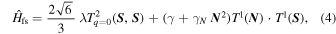
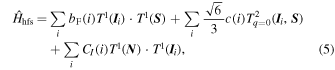
where λ is the electron spin–spin interaction parameter, whereas γ and γ_N are the electron spin–rotation constant and its centrifugal distortion term, respectively. The constants b_F and c describe the isotropic (Fermi contact interaction) and the anisotropic parts of the electron spin–nuclear spin coupling. C_I is the nuclear spin–rotation parameter. The index i runs over the ${}^{1}{\rm{H}}$ and ${}^{15}{\rm{N}}$ nuclei. The subscript q denotes the spherical component of the reference system attached to the molecular frame. Equations (3)–(5) only describe the energy contributions that are relevant for the present spectral analysis. The nuclear spin–nuclear spin hyperfine constants cannot be determined from the available data set, thus the corresponding terms have not been included in ${\hat{H}}_{\mathrm{hfs}}$

An overview of the fine and hyperfine pattern of the $N=1\leftarrow 0$ rotational transition is shown in Figure 1; each group of ${F}_{1}^{{\prime} },F^{\prime} \leftarrow {F}_{1},F$ hyperfine components is spread over ∼150 MHz, and the strongest lines are those with ${\rm{\Delta }}F={\rm{\Delta }}{F}_{1}={\rm{\Delta }}J$. The $N=1\leftarrow 0,J=0\leftarrow 1$ fine-structure components, located at 942 GHz, were previously recorded by Bailleux et al. (2012), whereas the other two components are first observed in this study.

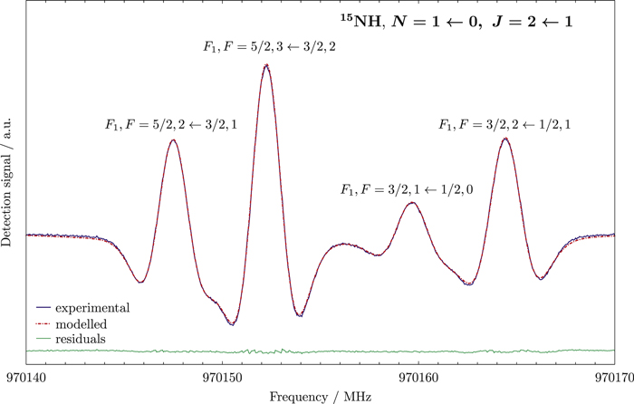
Zoom In Zoom Out Reset image size

The FWHM of the observed lines is about 2.5 MHz, because of the sizable Doppler broadening in this spectral range (∼1.8 MHz at 100 K). Thus, care had to be taken to retrieve accurate values of the corresponding central frequencies. We modeled the recorded absorption profiles using the proFFiT line analysis code (Dore 2003), adopting an FM Voigt profile function, and taking into account the full complex representation of the Fourier-transformed dipole correlation function. The imaginary dispersion term accounts for the line asymmetry produced by the spectral background and helps to obtain a cleaner determination of the central frequency. In total, 26 line positions have been accurately determined with this method; they include 22 newly measured frequencies plus the remeasurement of the four data previously reported by Bailleux et al. (2012). An example of the results obtained using proFFiT is presented in Figure 2, which shows the four strongest transitions of the $J=2\leftarrow 1$ fine-structure component.

Zoom In Zoom Out Reset image size

The content of the improved data set for ${}^{15}\mathrm{NH}$ is illustrated in Table 1. In the third column, the present measurements are listed, whereas the last column reports Table 2 of Bailleux et al. (2012) for comparison. For the $J=0\leftarrow 1$ lines, the discrepancies between the present and the older measurements are well within the estimated experimental uncertainties, with a maximum deviation of 64 kHz. Larger discrepancies were observed for the $J=2\leftarrow 1$ and $J=1\leftarrow 1$ fine-structure groups, whose components deviate from the predicted positions by ∼0.4 MHz and ∼2.5 MHz, respectively.

Table 1.  Measured Transition Frequencies^a (MHz) and Least-squares Residuals for the $N=1\leftarrow 0$ Transitions of ¹⁵NH in the Ground Vibrational State

$J^{\prime} \leftarrow J$	${F}_{1}^{{\prime} },F^{\prime} \leftarrow {F}_{1},F$	This Work	Fit o.−c.	Bailleux et al. (2012)
0 ← 1	1/2, 1 ← 1/2, 0	942037.007(35)	−0.001	942036.954(100)
	1/2, 1 ← 3/2, 1	942070.538(35)b	0.017c	942070.537(100)b
	1/2, 0 ← 3/2, 1	942070.538(35)b	0.017c	942070.537(100)b
	1/2, 1 ← 1/2, 1	942143.526(35)b	0.008c	942143.471(100)b
	1/2, 0 ← 1/2, 1	942143.526(35)b	0.008c	942143.471(100)b
	1/2, 1 ← 3/2, 2	942176.869(35)	−0.024	942176.923(100)
2 ← 1	5/2, 2 ← 3/2, 1	970147.498(35)	0.030	970147.73(50)d
	5/2, 3 ← 3/2, 2	970152.248(35)	−0.052	970152.62(50)d
	3/2, 1 ← 1/2, 0	970159.678(35)	0.023	970159.93(50)d
	3/2, 2 ← 1/2, 1	970164.444(35)	−0.042	970164.82(50)d
	3/2, 1 ← 3/2, 1	970193.161(35)	0.019	970193.48(50)d
	3/2, 2 ← 3/2, 2	970197.939(35)	−0.036	970198.36(50)d
	5/2, 2 ← 1/2, 1	970220.406(35)	0.030
	5/2, 2 ← 3/2, 2	970253.877(35)	0.012	970254.16(50)d
	3/2, 1 ← 1/2, 1	970266.067(35)	0.016	970266.36(50)d
1 ← 1	1/2, 1 ← 1/2, 0	995536.733(35)	−0.010	995534.36(90)d
	3/2, 1 ← 1/2, 0	995567.838(35)	−0.002	995565.57(90)d
	1/2, 1 ← 3/2, 1	995570.177(35)	−0.054
	1/2, 0 ← 3/2, 1	995574.075(35)	0.054	995571.81(90)d
	3/2, 2 ← 3/2, 1	995597.456(35)	0.039	995595.05(90)d
	3/2, 1 ← 3/2, 1	995601.361(35)	0.016	995599.11(90)d
	1/2, 1 ← 1/2, 1	995643.101(35)	−0.038	995640.79(90)d
	1/2, 0 ← 1/2, 1	995646.957(35)	0.027	995644.70(90)d
	3/2, 2 ← 1/2, 1	995670.300(35)	−0.025	995667.94(90)d
	3/2, 1 ← 1/2, 1	995674.240(35)	−0.014	995671.99(90)d
	1/2, 1 ← 3/2, 2	995676.663(35)	0.034	995674.33(90)d
	3/2, 2 ← 3/2, 2	995703.824(35)	0.010	995701.48(90)d
	1/2, 1 ← 3/2, 2	995707.720(35)	−0.023	995705.54(90)d

Notes.

^aNumbers in parentheses are the estimated experimental accuracies in units of the last quoted digit. ^bBlended transitions. ^cDeviation computed from the average frequency of the blend. ^dPredicted frequency and 1σ estimated error.

Download table as:  ASCIITypeset image

In the present experiment, we were also able to record 16 lines belonging to the $N=1\leftarrow 0$ transition on ${}^{15}\mathrm{NH}$ in its v = 1 vibrationally excited state (see Table 2). This excited level is located at an energy of ca. 3200 ${\mathrm{cm}}^{-1}$ above the ground state (∼4600 K), but it is appreciably populated even at 100 K because the plasma employed to produce the species is vibrationally hot (Dore et al. 2011).

Table 2.  Measured Transition Frequencies^a (MHz) and Least-squares Residuals for the $N=1\leftarrow 0$ Transitions of ¹⁵NH in the v = 1 Vibrational State

$J^{\prime} \leftarrow J$	${F}_{1}^{{\prime} },F^{\prime} \leftarrow {F}_{1},F$	This Work	Fit o.−c.
0 ← 1	1/2, 1 ← 1/2, 1	903477.713(35)b	0.000c
	1/2, 0 ← 1/2, 1	903477.713(35)b	0.000c
2 ← 1	5/2, 2 ← 3/2, 1	931714.698(35)	0.043
	5/2, 3 ← 3/2, 2	931720.767(35)	−0.080
	3/2, 1 ← 1/2, 0	931726.663(35)	0.020
	3/2, 2 ← 1/2, 1	931732.791(35)	−0.053
	3/2, 1 ← 3/2, 1	931759.349(35)	0.024
	5/2, 2 ← 3/2, 2	931826.352(35)	0.055
1 ← 1	1/2, 1 ← 1/2, 0	956924.228(35)	−0.001
	3/2, 1 ← 1/2, 0	956959.623(35)	0.000
	1/2, 0 ← 3/2, 1	956964.989(35)	0.053
	3/2, 2 ← 3/2, 1	956984.157(35)	0.040
	3/2, 1 ← 3/2, 1	956992.256(35)	−0.039
	1/2, 1 ← 1/2, 1	957035.839(35)	−0.029
	1/2, 1 ← 3/2, 2	957068.514(35)	−0.026
	3/2, 1 ← 1/2, 1	957071.296(35)	0.032
	3/2, 2 ← 3/2, 2	957095.727(35)	−0.032

Notes.

^aNumbers in parentheses are the estimated experimental accuracies in units of the last quoted digit. ^bBlended transitions. ^cDeviation computed from the average frequency of the blend.

Download table as:  ASCIITypeset image

The spectral analysis was performed considering the complete rotational data set available for ${}^{15}\mathrm{NH}$, which comprises our new measurements and the FIR data reported by Bailleux et al. (2012). The different precisions were taken into account by assigning to each ith entry a weight, w_i, that is inversely proportional to the square of its estimated measurement uncertainty, ${w}_{i}=1/{\sigma }_{i}^{2}$. For the present spectra, 35 kHz was adopted as the average measurement error. This was estimated by repeated profile analyses with proFFiT using different sets of fitting parameters and background subtraction techniques. For the literature FIR data taken at SOLEIL, we retained the original value of 1 × 10⁻⁴ ${\mathrm{cm}}^{-1}$ (3 MHz).

The transition frequencies were fitted to the Hamiltonian parameters described by Equations (3)–(5) using the spfit analysis program (Pickett 1991). Eleven spectroscopic parameters were determined for the ground vibrational state and they include: the rotational and centrifugal distortion constants, B, D, and H; the spin–spin interaction coefficient, λ; the spin–rotation constant, γ, together with its N² centrifugal correction, γ_N; the full set of electron spin–nuclear spin interaction constants for ${}^{15}{\rm{N}}$ and D, b_F, c; and the nuclear rotation–nuclear spin coupling coefficient for nitrogen, C_I. Not all of these Hamiltonian coefficients could be adjusted for the v = 1 state because the set of detected hyperfine components is smaller, hence suitable constraints had to be adopted for the indeterminable spectroscopic parameters. They were obtained from the corresponding ground state values corrected for the $v=0\leftrightarrow 1$ vibrational dependence, as estimated from ¹⁴NH literature data (Ram et al. 1999; Lewen et al. 2004) The two sets of constants for the v = 0 and v = 1 states are reported in Table 3, where the previous results obtained by Bailleux et al. (2012) are also shown for comparison.

Table 3.  Spectroscopic Parameters Derived for ¹⁵NH

Constanta	Units	v = 0	v = 1	Bailleux et al. (2012)
B	/MHz	487799.053(11)	468536.3401(51)	487798.75(15)
D	/MHz	50.5977(52)	49.9514b	50.591(6)
H	/kHz	3.657(77)	3.488b	3.61(6)
L	/Hz	−0.4035c	−0.4020b	−0.4035
λ	/MHz	27577.650(10)	27564.616(18)	27576.15(63)
γ	/MHz	−1637.235(22)	−1551.167(10)	−1636.53(36)
γJ	/MHz	0.443(11)	0.402b	0.4389
${b}_{F}({\rm{H}})$	/MHz	−66.074(10)	−69.876(15)	−66.085(29)
$c({\rm{H}})$	/MHz	90.546(44)	87.065(53)	90.285d
${b}_{F}{(}^{15}{\rm{N}})$	/MHz	−26.416(13)	−25.554(19)	−26.462(35)
$c{(}^{15}{\rm{N}})$	/MHz	95.283(44)	94.613(54)	95.331d
$C{(}^{15}{\rm{N}})$	/MHz	−0.211(21)	−0.129(24)	−0.223
no. of lines		43	16	21
σwe		0.835		⋯

Notes.

^aNumbers in parentheses are the 1σ errors in units of the last quoted digit. ^bConstrained. See the text. ^cFixed at the value reported for ¹⁴NH (Lewen et al. 2004). ^dDerived from $t=c/3$. ^eWeighted root mean square deviation of the fit.

Download table as:  ASCIITypeset image

The spectroscopic constants determined in the present work are consistent with the ones previously reported by Bailleux et al. (2012), but their precision has been improved substantially. The rotational parameters, B and D, and the spin–rotation constant, γ, have had their standard uncertainty reduced by one order of magnitude, and major improvements were also achieved for the sextic centrifugal distortion constant, H, and for the spin–spin interaction parameter, λ. New determinations of the dipolar spin–spin hyperfine coefficients, c, for both H and ${}^{15}{\rm{N}}$ were also obtained. In the previous work, these parameters were not adjusted; $c({\rm{H}})$ was fixed at the value of the parent ${}^{14}\mathrm{NH}$ species, whereas c(${}^{15}{\rm{N}}$) was constrained to a value obtained from the ${}^{14}\mathrm{NH}$ datum multiplied by the ${}^{15}{\rm{N}}$/${}^{14}{\rm{N}}$ nuclear magnetogyric ratio (Bailleux et al. 2012). Our results are in good agreement with these figures with discrepancies that do not exceed 0.5%. We have also determined the small nuclear spin–rotation constant C_I for ${}^{15}{\rm{N}}$ to a precision of 10%, and its experimental value compares well with the one derived from the main isotopologue using the same scaling relation described above.

From the fit of the v = 1 lines, we have derived B, D, λ, γ, the Fermi contact (b_F), and dipolar spin–spin (c) hyperfine constants for both nuclei. The observed difference of these coefficients with respect to the corresponding ground state (v = 0) values are within the range expected for a regular vibrational dependence: ∼5% for the hyperfine constants, >0.1% for the spin–spin constant λ, and 3%–6% for the rotational constant B and for the spin–rotation constant γ. From these latter parameters, one can estimate the value of the corresponding first-order vibrational dependence coefficients:

$$\begin{eqnarray}&&{\alpha }_{e}\approx B(v=0)-B(v=1),\end{eqnarray} \tag{ 6a }$$

$$\begin{eqnarray}&&{\rm{\Delta }}\gamma \approx \gamma (v=0)-\gamma (v=1).\end{eqnarray} \tag{ 6b }$$

These can be compared to the value obtained from the ${}^{14}\mathrm{NH}$ isotopologue using the mass–scaling relation (Ross et al. 1974; Watson 1980), neglecting the Born–Oppenheimer breakdown effects:

$$\begin{eqnarray}&&{\alpha }_{e}{(}^{15}\mathrm{NH})\approx {\alpha }_{e}{(}^{14}\mathrm{NH}){\left(\displaystyle \frac{{\mu }_{{}^{14}\mathrm{NH}}}{{\mu }_{{}^{15}\mathrm{NH}}}\right)}^{3/2},\end{eqnarray} \tag{ 7a }$$

$$\begin{eqnarray}&&{\rm{\Delta }}\gamma {(}^{15}\mathrm{NH})\approx {\rm{\Delta }}\gamma {(}^{14}\mathrm{NH}){\left(\displaystyle \frac{{\mu }_{{}^{14}\mathrm{NH}}}{{\mu }_{{}^{15}\mathrm{NH}}}\right)}^{3/2},\end{eqnarray} \tag{ 7b }$$

where μ is the reduced mass of the two isotopologues. Using the results reported by Ram et al. (1999) for ${}^{14}\mathrm{NH}$, from Equation (7a), one obtains ${\alpha }_{e}{(}^{15}\mathrm{NH})=19262.7\,\mathrm{MHz}$ and ${\rm{\Delta }}\gamma {(}^{15}\mathrm{NH})=-91.7$ MHz. These values are in good agreement with our experimentally determined ones, which are 19261.4 MHz and −86.1 MHz, respectively.

The observation of spectral features belonging to the v = 1 vibrationally excited state implies that collisions in the low-pressure plasma employed in the present experiment to produce ${}^{15}\mathrm{NH}$ are efficient enough to populate the bottom part of its vibrational ladder. The vibrational temperature of the plasma can be roughly estimated by comparing the intensity of the strongest $J,{F}_{1},F=2,5/2,3\leftarrow 1,3/2,2$ hyperfine components recorded for both the ground and the v = 1 states under the same experimental conditions. The intensity ratio was found to be ∼1/40. Using the harmonic wavenumber of the N–H stretch reported by Ram et al. (1999) for ${}^{14}\mathrm{NH}$(ω = 3282.7 ${\mathrm{cm}}^{-1}$) and assuming Boltzmann populations, one can estimate a vibrational temperature of ${T}_{\mathrm{vib}}\sim 1270$ K.

Here, we report on the first complete laboratory study of the $N=1\leftarrow 0$ rotational transition of the astrophysically important ${}^{15}\mathrm{NH}$ radical in its ${X}^{3}{{\rm{\Sigma }}}^{+}$ ground electronic states. This fundamental rotational transition is split into three main fine components, each with a wide-spread hyperfine structure. The strongest features belong to the $J=2\leftarrow 1$ and $J=1\leftarrow 1$ components, which we have observed for the first time. Only a few submillimeter measurements were previously available (four components of the $J=0\leftarrow 1$ group recorded by Bailleux et al. 2012). This study substantially improves the knowledge of the THz spectrum of ${}^{15}\mathrm{NH}$. Accurate values of the central line position (σ ∼ 35 kHz, ≈0.01 km s⁻¹) were determined via a line profile analysis of 25 components of the ground state and 16 components of the v = 1 vibrationally excited state. These improved data can be used for Herschel archival searches, as a guidance for sensitive observations with 4GREAT instrument on board SOFIA, and for future THz telescopes.

This work was supported by Italian MIUR (PRIN 2015 "STARS in the CAOS") and by the University of Bologna (RFO funds).