


Abstract
The shear and cohesive strengths of a rubble-pile asteroid could influence the critical spin at which the body fails and its subsequent evolution. We present results using a soft-sphere discrete element method to explore the mechanical properties and dynamical behaviors of self-gravitating rubble piles experiencing increasing rotational centrifugal forces. A comprehensive contact model incorporating translational and rotational friction and van der Waals cohesive interactions is developed to simulate rubble-pile asteroids. It is observed that the critical spin depends strongly on both the frictional and cohesive forces between particles in contact; however, the failure behaviors only show dependence on the cohesive force. As cohesion increases, the deformation of the simulated body prior to disruption is diminished, the disruption process is more abrupt, and the component size of the fissioned material is increased. When the cohesive strength is high enough, the body can disaggregate into similar-size fragments, which could be a plausible mechanism to form asteroid pairs or active asteroids. The size distribution and velocity dispersion of the fragments in high-cohesion simulations show similarities to the disintegrating asteroid P/2013 R3, indicating that this asteroid may possess comparable cohesion in its structure and experience rotational fission in a similar manner. Additionally, we propose a method for estimating a rubble pile's friction angle and bulk cohesion from spin-up numerical experiments, which provides the opportunity for making quantitative comparisons with continuum theory. The results show that the present technique has great potential for predicting the behaviors and estimating the material strengths of cohesive rubble-pile asteroids.
Export citation and abstract BibTeX RIS
1. Introduction
Growing evidence suggests that asteroids larger than a few hundred meters in diameter are gravitational aggregates, i.e., they are rubble-pile asteroids for which gravity is the principal force holding the body together (Richardson et al. 2002; Michel et al. 2015). However, because the gravity is so small on these minor bodies, the physical interactions arising from other sources may also play a significant role on their mechanical behaviors. Scheeres et al. (2010) analyzed a number of physical effects that may act on particles on asteroid surfaces, among which the van der Waals cohesive force should be a dominant force and could be comparable to the gravity. The mechanism of the interparticle van der Waals cohesive force is associated with molecular or atomic polarization effects, which become important for particles with size on the order of several micrometers (Israclachvili 1985). Given that the regolith sample of asteroid 25143 Itokawa returned by the Hayabusa spacecraft has a size distribution of ∼10 to ∼100 μm (Nakamura et al. 2011), it is appropriate to consider the existence of the van der Waals cohesive force in asteroid bodies, and assess whether these forces will be important to their evolution. In addition, the ultra-high vacuum space environment that improves the surface cleanliness of individual particles can enhance the van der Waals interaction, causing it to be non-negligible even for larger particles (Perko et al. 2001). Based on the morphology of the asteroid Itokawa, Sánchez & Scheeres (2014) suggest that rubble-pile asteroids could be made of meter-sized boulders that are connected through smaller interstitial grains (i.e., granular bridges) that are themselves linked by cohesive interactions.
The existence of cohesive forces can increase the tensile strength of rubble-pile asteroids and prevent their breakup by rotational centrifugal forces (Holsapple 2007; Sánchez & Scheeres 2014, 2016). In turn, study of the spin limit of asteroids can shed light on their internal structure, strengths (shear and cohesive), and evolution processes (Hirabayashi 2015; Zhang et al. 2017). From the spin rate distribution of 688 asteroids, Harris (1996) noted that no asteroids spin faster than the spin barrier for a bulk density of ∼2.7 g/cc, above which equatorial material cannot remain bound against centrifugal acceleration, suggesting a cohesionless rubble-pile structure for asteroids larger than ∼300 m in diameter. Subsequent observations of spin states of thousands of asteroids show similar results (e.g., Pravec & Harris 2000; Pravec et al. 2002a). However, based on elastic-plastic continuum theory for solid materials, Holsapple (2001, 2004) pointed out that the spin limit is constrained by the material shear strength of asteroids, with lower strength leading to a narrower region of permissible equilibrium spin states. If the strength of asteroid materials is similar to that of terrestrial cohesionless sand, some asteroids may have already violated their spin limits. Furthermore, recent observations show that a handful of asteroids can spin significantly faster than the spin barrier, e.g., asteroid (455213) 2001 OE84 (Pravec et al. 2002b; Polishook et al. 2017), asteroid (335433) 2005 UW163 (Chang et al. 2014), asteroid (60716) 2000 GD65 (Polishook et al. 2016), and asteroid (144977) 2005 EC127 (Chang et al. 2017). The dynamical and collisional evolution histories make these asteroids unlikely to be monolithic structures (e.g., Michel et al. 2015; Polishook et al. 2016), while a cohesive rubble-pile structure can well explain these fast rotators. Furthermore, the disruption events observed for some active asteroids (e.g., main-belt asteroid P/2013; Jewitt et al. 2014) also indicate the existence of cohesion (Hirabayashi et al. 2014; Jewitt et al. 2017).
The main objective of this paper is to infer the dependence of the spin limits and failure behaviors of rubble-pile asteroids on the shear and cohesive strengths. Our effort builds upon a first investigation that assesses the behaviors of rubble-pile asteroids without cohesion (Zhang et al. 2017). Theoretical efforts have been carried out to explore the consequence of cohesion on spin limits and failure (e.g., Holsapple 2007; Hirabayashi 2015). When the shape, mass bulk density, and spin rate of an asteroid are known, the level of cohesive strength needed to keep the body bound together can be estimated from the closed-form algebraic formulas derived by Holsapple (2007). This theory has been successfully applied to several real asteroids. For example, the 2-km-diameter main-belt asteroid (60716) 2000 GD65 can maintain global stability at a spin period of 1.9529 hr with cohesion of 150–450 Pa (Polishook et al. 2016), and the 1-km-diameter near-Earth asteroid (29075) 1950 DA only needs a cohesive strength of ∼64 Pa to be stable at its current observed spin period of 2.1216 hr (Rozitis et al. 2014). Both values are within the range of the cohesive strength measured for weak lunar regolith (Mitchell et al. 1972). By analyzing the elastic stress distribution in a spherical body, Hirabayashi (2015) found that the failed regions in such a body move from the equatorial surface to the center as the spin rate increases, implying transition of the failure mode from surface failure to interior failure. However, our previous study shows that the microscopic heterogeneity generated by arranging discrete particles within a rubble pile can significantly influence the shear strength and failure behaviors of spinning rubble piles (Zhang et al. 2017). Given the discrete nature of the rubble-pile structure, continuum models may not be well adapted to fully characterize the mechanical behavior of rubble-pile asteroids.
As an important numerical technique in granular material research, the Soft-Sphere Discrete Element Method (SSDEM) complements continuum modeling efforts. SSDEM numerical investigations on behaviors of rubble-pile bodies during spin-up processes have given intriguing insights into the effect of interactions between particles. Sánchez & Scheeres (2012) explored the effect of interparticle sliding friction on the failure modes of cohesionless ellipsoids, and confirmed the consistency of the reshaping process in simulation with the continuum theory (i.e., Holsapple 2010). With the implementation of a physically based contact model incorporating rotational resistances, Zhang et al. (2017) found that the failure mode of a cohesionless rubble pile depends mainly on the arrangement and size distribution of its constituent particles. For cohesive bodies, Sánchez & Scheeres (2016) observed that large components can be rapidly detached from the simulated rubble pile when the cohesive strength is high enough. Hirabayashi et al. (2015) found that the heterogeneous distribution of cohesion can change the failure mode of a rubble pile. All of these studies indicate the positive roles of interparticle friction and cohesion in changing the failure spin rate of rubble-pile bodies. Despite these efforts, the contributions to the material strengths of a rubble pile of the sliding and rotational friction as well as the cohesion in the SSDEM contact model is still poorly understood. Furthermore, it is hard to make comparisons with the continuum theory due to lack of proper quantitative analyses on the macroscopic strength parameters (i.e., the friction angle and the cohesive strength used in the failure criterion for granular materials; see Section 3.2) in these studies.
In this paper, we use a high-efficiency SSDEM code, pkdgrav, to investigate the mechanical properties and dynamical behaviors of cohesive self-gravitating rubble piles subject to increasing rotational centrifugal forces and explore their spin limits. Analyses at three different scales, i.e., the global (full-body) scale, the macroscopic (representative volume elements) scale, and the microscopic (particle-level) scale, are carried out to reveal the details of simulated bodies during spin-up processes. Following the granular bridge idea proposed by Sánchez & Scheeres (2014, 2016), we develop a comprehensive contact model incorporating translational and rotational friction and van der Waals interactions arising from interstitial fine grains to simulate cohesive granular materials, and design three SSDEM parameters to control the interparticle frictional and cohesive strengths (see Section 2). A series of numerical triaxial compression tests are carried out to measure the performance of the contact model and calibrate the mechanical properties of the simulated granular specimen with those obtained in laboratory experiments (see Section 3). Then, we explore the effects of the three SSDEM parameters on the behaviors of rubble piles during spin-up processes in Section 4. In Section 5, a method from a granular mechanics perspective is proposed to estimate the spin limit and macroscopic material strengths of a simulated rubble pile. Finally, Section 6 presents comparisons of our simulation results with the continuum theory and discusses the implications.
2. SSDEM with Cohesion
2.1. Basic Features of SSDEM Implemented in pkdgrav
In a granular assembly, each particle can interact with its surroundings through short-range interactions (e.g., mechanical contact forces, van der Waals forces) and long-range interactions (e.g., gravity, electrostatic forces).7
Within the high-efficiency parallel tree code framework, pkdgrav (Richardson et al. 2000; Stadel 2001), a soft-sphere model including four components in the normal, tangential, rolling, and twisting directions is used for computing particle contact forces (Schwartz et al. 2012; Zhang et al. 2017). Figure 1 presents the directions of the forces and torques acting on particle i generated by the contact with particle j. The linear spring-dashpot normal contact force  and the tangential stick-slip force
  are given by


which depend on the stiffness constants, kN and kS, the viscous damping coefficients, CN and CS, and the sliding friction coefficient μS.8
The variable δN is the mutual compression between two particles, and  is the sliding displacement from the equilibrium contact point. The unit vector
  gives the direction from the center of particle i to that of particle j. The dashpot force is linearly proportional to the normal and tangential relative velocities,
  and
and  . Recently, in order to capture behaviors of granular materials under quasi-static loadings, a spring-dashpot-slider rotational resistance model was implemented in pkdgrav (Zhang et al. 2017). The resulting rolling and twisting torques,
  and
and  , are given by
where kR and kT are the material stiffness along rolling and twisting directions, and CR and CT are the damping coefficients for rolling and twisting motions.  and
and  describe the relative rolling and twisting motions between two particles in contact. Similar to the tangential force model,
  and
and  are the rolling and twisting angular displacements from the equilibrium contact point, respectively. When the magnitude of the rolling/twisting torque reaches a critical value, MR,max or MT,max, the surfaces of the two particles start to slide relative to each other along the rolling/twisting direction, whereupon the system enters into a dynamic friction condition. The motion of a particle can be obtained by integrating the total force and torque acting on it.

Figure 1. Schematic of transmitted forces and torques at a contact in a local Cartesian coordinate system, where  and
and  are in the contact plane and
  is in the normal direction according to the right-hand rule. The two irregular convex polyhedrons represent the Voronoi tessellation (which divides the space containing all particles into subdomains, one per particle, where each subdomain consists of all points closer to its particle than any other; the open-source library Voro++ introduced by Rycroft 2009, can be used to build the Voronoi tessellation for granular assemblies) for particle i and j in a granular assembly, where the orange polygon represents the power plane (every point in this plane has the same distance to the surfaces of particles i and j, which is closer than the distance to any other particles' surfaces) of these two neighboring particles. The dashed yellow circle on the contact plane (exaggerated for illustration) denotes the actual contact area.
Download figure:
Standard image High-resolution imageThe interactions between particles and wall boundaries with a wide range of geometries as well as the effect of gravity are also implemented in pkdgrav, allowing precise reproduction of laboratory experiments (see Schwartz et al. 2012 for details). The numerical approach has been validated through comparison with laboratory experiments, e.g., low-speed impact experiments (Schwartz et al. 2014), and has been successfully used to study various behaviors of granular systems, e.g., the Brazil-nut effect (Matsumura et al. 2014; Perera et al. 2016; Maurel et al. 2017) and avalanches (Yu et al. 2014). In addition, the parallel hierarchical tree code in pkdgrav provides a highly efficient way to carry out long-range interaction calculations for an N-body system, giving an  scaling dependence, where N is the number of particles in a simulation (Richardson et al. 2000). With the current processing power, pkdgrav has the ability to simulate the evolution of tens of thousands to millions of particles; this has been well tested in a wide range of environments (e.g., Ballouz et al. 2015, 2017; Zhang et al. 2017; Schwartz et al. 2018).
2.2. Cohesive Normal Force
Several cohesion models have been implemented previously in pkdgrav, but for a different cohesive mechanism, i.e., sintering forces, which can build very strong bonds giving rise to the formation of particle aggregates (see Richardson et al. 2009; Schwartz et al. 2013). Although the thermal processes on asteroids may facilitate the formation of sintering bonds between grains at the asteroids' surface, the van der Waals force is a more universal mechanism for bodies in a low-gravity, ultra-high-vacuum environment (Scheeres et al. 2010), which has been verified for lunar regolith (Mitchell et al. 1972).
The cohesive force introduced in this study is a combination of the granular bridge idea proposed by Sánchez & Scheeres (2014, 2016) and a hypothetical contact area characterized by a shape parameter, β, first introduced in the contact model of Jiang et al. (2013, 2015). With the assumption that there exist substantial micro-sized grains to cover larger boulders, this model can mimic the cumulative effect of the cohesive regolith between two large boulders without simulating each individual fine grain. The rotational resistance arising from the interstitial regolith is also taken into account via the hypothetical contact area.
As shown in Figure 1, taking particles i and j as boulder representatives and assuming that there are many fine particles distributed around the gaps between these two boulders to form a granular bridge, we can obtain the cumulative forces and torques transmitted through the granular bridge by integration over an effective contact area. The orange polygon shown in Figure 1 can serve as the effective contact area that contains all the points that are at the same distance from the two boulders' surfaces and are closer than these surfaces to any other boulders' surfaces. The area of this polygon can be accurately calculated using the Voronoi tessellation per pair of neighboring boulders in principle. To avoid this burdensome calculation, we introduce the shape parameter, β, to represent a statistical measure of the area where the interstitial grains are important and approximate this effective contact area using a rectangle:

where the effective radius R = rirj/(ri + rj), and ri and rj are the radii of the corresponding boulders. The resulting cohesive force between the two boulders can be modeled as

where the interparticle cohesive tensile strength c reflects the physical properties of the interstitial regolith, e.g., porosity, size distribution, surface energy, and Hamaker constants (Seizinger et al. 2013; Sánchez & Scheeres 2014; Gundlach & Blum 2015).
The interstitial cohesive regolith will also strengthen the friction between boulders to resist relative rotational motion, commensurate with the shape effect (Li et al. 2011; Jiang et al. 2013). With a similar contact area characterized by the shape parameter β, the rolling/twisting stiffness and damping coefficients can be expressed as

When the relative rolling/twisting rotational motion exceeds a critical threshold, the cohesive contact on the edge of the contact area begins to break, and the peak rolling/twisting torque is given as

where μR and μT represent the static friction coefficients for rolling and twisting, respectively.9
In our implementation, the cohesive force described in Equation (4) is added to the calculation of the interaction between two particles in contact, and is ignored when the two particles are separated. By these means, the breakage and recovery of the cohesive effect of interstitial regolith can be captured. Although the behavior of individual interstitial grains is not physically simulated, our model can capture the resulting tensile strength and rotational resistances well, which is sufficient for our purpose of demonstrating the effect of cohesive strength on rubble-pile asteroids. In addition, since the effective contact area Aeff given by Equation (3) could be much larger than the actual contact area between two spherical particles (i.e., the dashed yellow circle shown in Figure 1), the resulting rotational resistance and cohesion can reduce excess particle rotations and restrict the particles' freedom to rotate. Therefore, the effects of surface roughness and the interlocking of non-spherical shapes found for real-world granular materials can be reflected to some extent in our model. In Section 3, a series of drained triaxial compression tests were carried out to validate the ability of our SSDEM model to simulate cohesive granular materials.
2.3. Parameter Setup of SSDEM
Before proceeding to lay out numerical simulations, it is necessary to clarify how we set the parameters used in our SSDEM model, including two stiffness constants, kN and kS, two damping coefficients, CN and CS, three friction coefficients, (μS, μR, μT), a shape parameter β, an interparticle cohesive tensile strength c, and an integration timestep Δt. The normal stiffness kN and the timestep Δt are set to ensure that particle overlaps for each entire simulation do not exceed 1% of the minimum particle radius (in cases where it is important to match the sound speed of real materials, kN can also be chosen to control the speed of energy propagation through a medium represented by soft-sphere particles; see Section 2.1 in Schwartz et al. 2012 for details). To keep normal and tangential oscillation frequencies equal to each other, the tangential stiffness kS is often set to (2/7)kN (see Section 2.6 in Schwartz et al. 2012, for details). CN and CS can be derived from the normal and tangential coefficients of restitution, εN and εS, which are set to 0.55 so that the granular system is subject to sufficient damping (these values are also reasonable for terrestrial rocks; Chau et al. 2002). μR and μT represent the capability of the interstitial regolith to resist breakage, which are set to 1.3 and 1.05 for a medium level, respectively (the derivation is similar to the cohesionless case; we refer the reader to Jiang et al. 2015, for details).
By these means, the dimension of the SSDEM parameter space is narrowed down to three, i.e., μS, β, and c, which control the sliding resistance strength, the rotational resistance strength, and the cohesive strength between particles in contact, respectively. In SSDEM simulations, these three parameters can serve as the adjustable material parameters, allowing the modeling of granular materials with various material properties, as revealed in the following section.
3. SSDEM Calibration: Triaxial Compression Tests
The drained triaxial compression test is a common method to measure the mechanical properties of granular materials (Lade 2016). Here, the same procedure is applied to calibrate the properties of the simulated specimen using our SSDEM model against that of real sand.
3.1. Simulation Setup
Figure 2 illustrates the simulation setup. The triaxial compression procedure is automatically performed using pkdgrav. In the beginning, a uniform confining pressure is applied to the specimen and then the vertical axial strain ε1 is increased linearly in compression while the motions of the lateral walls are controlled by a servo mechanism that can maintain a constant confining pressure continuously acting on the specimen, i.e., σ2 = σ3 = constant.10 To meet quasi-static loading conditions, the top and bottom walls are moved toward each other at a constant strain rate of 3% per minute.
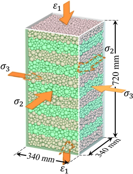
Figure 2. Schematic of a triaxial test simulated using SSDEM. During loading, the pressures acting on the lateral walls remain constant (σ2 = σ3), and the vertical strain ε1 is linearly increased in compression (the layers are colored for illustration only).
Download figure:
Standard image High-resolution imageThe granular specimen used in our triaxial tests consists of ∼14,000 particles, with a −3-index power-law distribution in radius ranging from 6 mm to 18 mm and a material density of 3.0 g/cc. A two-stage procedure is used to prepare the specimen for representing the macroscopic homogeneity of a real sand sample (the same procedure is also applied to generate rubble-pile asteroid representatives in Section 4).11 First, a granular assembly is created by placing particles with a predefined size distribution randomly in a spherical cloud and allowing the cloud to gravitationally collapse with highly inelastic collisions. Frictionless and cohesionless SSDEM parameters are used to minimize the void space between particles. Second, a portion with a predefined shape is extracted from the interior of the granular assembly produced in the first step.
The prepared specimen is isotropically compressed to a uniform confining pressure condition in a 340 mm × 340 mm × 720 mm box with six frictionless boundary walls (see Figure 2). Given that the particle arrangement is sensitive to the external gravity field, leading to a biased direction of the contact forces, compression processes (including the isotropic and triaxial) are conducted in a gravity-free condition. Figure 3 presents the distribution of contact orientations prior to vertical loading, showing that this specimen is virtually homogeneous in all directions. The packing efficiency of our tested sample is ∼0.62, which is within the typical range of terrestrial sands observed in laboratory tests (Cabalar et al. 2013).
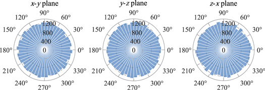
Figure 3. Distribution of the contact orientations of a specimen under a uniform confining pressure. The contact normal vectors are projected on x–y, y–z, and z–x planes. The length of each sector is the number of contacts in each directional interval (7.5°), and the sum of the sector lengths is the total contact number of this specimen.
Download figure:
Standard image High-resolution imageTo reproduce the desired elastic mechanical property and match the sound speed of real sand, a normal stiffness constant kN of 5.1 × 10⁶ kg s−2 is chosen (a stiffer kN normally leads to a higher Young's modulus), and the integration timestep Δt is set to 3.6 × 10⁻⁶ s so that particle overlaps for each entire simulation do not exceed 1% of the minimum particle radius. The effect of μS, β, and c is explored in Section 3.3.
3.2. Material Strength Determination: Drucker–Prager Failure Criterion
The material strengths of a granular material can be derived from its failure stress state. As one of the most common yield criteria for geophysical granular materials, the Drucker–Prager failure criterion has been successfully applied to analyzing the failure of rubble-pile structures (e.g., Holsapple 2007; Sharma et al. 2009; Hirabayashi 2015), which is given as (Jaeger et al. 2009)

where I1 is the first invariant of the Cauchy stress tensor, and J2 is the second invariant of the deviatoric stress tensor, which can be written in terms of the principal stresses, σ1, σ2, and σ3 (from largest to smallest), as I1 = σ1+σ2+σ3, ![${J}_{2}\,=[{({\sigma }_{1}-{\sigma }_{2})}^{2}+{({\sigma }_{2}-{\sigma }_{3})}^{2}+{({\sigma }_{3}-{\sigma }_{1})}^{2}]/6$](https://content.cld.iop.org/journals/0004-637X/857/1/15/revision1/apjaab5b2ieqn17.gif) .
.
The failure envelope (Equation (7) with the equality) plotted in the I1– plane is a straight line with a slope of s and an intercept of C, in which s and C represent the shear and cohesive strengths of the granular material, respectively, as shown in Figure 4. Note that this cohesive strength C represents the bulk property of the granular material, which is different from the interparticle cohesive tensile strength c used in the cohesive force model (Equation (4)). We distinguish this large C as the macroscopic cohesive strength. Since the Drucker–Prager failure envelope is a smooth version of the Mohr-Coulomb failure envelope, the slope s can be expressed as a function of the commonly used friction angle ϕ, i.e.,
 ![$s=2\sin \phi /[\sqrt{3}(3-\sin \phi )]$](https://content.cld.iop.org/journals/0004-637X/857/1/15/revision1/apjaab5b2ieqn19.gif) .
.
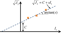
Figure 4. Determination of ϕ and C from triaxial compression tests. The crosses represent the results of triaxial compression tests under different confining pressures.
Download figure:
Standard image High-resolution imageThe constants ϕ and C can be determined from results of triaxial compression tests. Generally, three or more tests should be performed to make an appropriate estimation. As shown in Figure 4, the stress states at failure (i.e., the state at which the deviator stress achieves its peak in triaxial compression tests) under different confining pressure are plotted in the I1– plane, and a best-fit straight line (i.e., the failure envelope) can be derived from these data points. Then the values of ϕ and C can be extracted from the failure envelope.
3.3. Triaxial Simulation Results
The macroscopic mechanical properties of a specimen are characterized by four parameters, i.e., the friction angle ϕ, the macroscopic cohesive strength C, the Young's modulus E, and the Poisson's ratio ν. ϕ and C can be estimated using the method introduced in Section 3.2, and E and ν can be obtained from the initial slopes in the linear-elastic regime of the stress-strain curve and the volumetric strain curve, respectively (Belheine et al. 2009),

We investigated the effects of the SSDEM parameters, μS, β, and c, on these macroscopic properties. To draw the failure envelope, triaxial tests for each parameter set were conducted under three confining pressures, i.e., σ2 = σ3 = 50 kPa, 100 kPa, and 200 kPa, respectively. As shown in Table 1, the value ranges of the Young's modulus E and the Poisson's ratio ν and their dependences on the confining pressure are consistent with laboratory experiments on real sands (e.g., for the Labenne medium sand, E ∼ 100 MPa, ν ∼ 0.27, and ϕ ∼ 36°; see Kolymbas & Wu 1990; Mestat & Berthelon 2001), indicating the validity of our SSDEM model.
Table 1. Summary of Simulation Parameters (Second Column to Fifth Column) and Material Properties (Last Four Columns) That Were Estimated from Triaxial Compression Testsa
| Sim. No. | μS | β | c (kPa) | σ3 (kPa) | E (MPa) | ν | ϕ (°) | C (kPa)b |
|---|---|---|---|---|---|---|---|---|
| 50 | 76.8 | 0.303 | ||||||
| 1 | 0.3 | 0.3 | 0 | 100 | 100.5 | 0.277 | 30.3 ± 0.2 | −0.4 ± 1.1 |
| 200 | 124.6 | 0.232 | ||||||
| 50 | 84.3 | 0.283 | ||||||
| 2 | 0.3 | 0.5 | 0 | 100 | 109.2 | 0.257 | 32.0 ± 0.5 | −0.6 ± 2.9 |
| 200 | 131.6 | 0.221 | ||||||
| 50 | 88.8 | 0.273 | ||||||
| 3 | 0.3 | 0.7 | 0 | 100 | 113.9 | 0.246 | 32.4 ± 0.8 | 0.4 ± 4.3 |
| 200 | 135.9 | 0.213 | ||||||
| 50 | 92.2 | 0.265 | ||||||
| 4 | 0.3 | 1.0 | 0 | 100 | 117.7 | 0.238 | 32.3 ± 0.5 | 1.2 ± 3.1 |
| 200 | 139.6 | 0.206 | ||||||
| 50 | 92.9 | 0.275 | ||||||
| 5 | 0.5 | 0.3 | 0 | 100 | 111.6 | 0.258 | 37.1 ± 1.1 | −3.3 ± 7.2 |
| 200 | 130.0 | 0.229 | ||||||
| 50 | 105.2 | 0.249 | ||||||
| 6 | 0.5 | 0.5 | 0 | 100 | 121.9 | 0.237 | 40.6 ± 0.5 | −2.9 ± 3.6 |
| 200 | 137.1 | 0.216 | ||||||
| 50 | 107.9 | 0.244 | ||||||
| 7 | 0.5 | 0.7 | 0 | 100 | 125.2 | 0.231 | 42.4 ± 0.2 | −2.3 ± 1.9 |
| 200 | 141.2 | 0.208 | ||||||
| 50 | 112.5 | 0.234 | ||||||
| 8 | 0.5 | 1.0 | 0 | 100 | 129.9 | 0.222 | 43.9 ± 0.5 | −2.2 ± 4.2 |
| 200 | 145.4 | 0.201 | ||||||
| 50 | 105.1 | 0.262 | ||||||
| 9 | 1.0 | 0.3 | 0 | 100 | 119.2 | 0.251 | 44.2 ± 0.3 | −1.0 ± 2.9 |
| 200 | 132.1 | 0.227 | ||||||
| 50 | 114.0 | 0.243 | ||||||
| 10 | 1.0 | 0.5 | 0 | 100 | 127.1 | 0.235 | 49.3 ± 0.8 | −0.9 ± 5.8 |
| 200 | 138.9 | 0.215 | ||||||
| 50 | 119.7 | 0.231 | ||||||
| 11 | 1.0 | 0.7 | 0 | 100 | 131.9 | 0.225 | 52.7 ± 0.1 | −1.0 ± 1.5 |
| 200 | 142.9 | 0.207 | ||||||
| 50 | 124.8 | 0.220 | ||||||
| 12 | 1.0 | 1.0 | 0 | 100 | 136.1 | 0.215 | 56.3 ± 0.0 | 0.4 ± 0.2 |
| 200 | 146.9 | 0.200 | ||||||
| 50 | 106.3 | 0.251 | ||||||
| 13 | 0.5 | 0.5 | 31.4 | 100 | 122.4 | 0.239 | 41.5 ± 0.1 | 0.4 ± 0.6 |
| 200 | 137.2 | 0.216 | ||||||
| 50 | 111.7 | 0.243 | ||||||
| 14 | 0.5 | 0.5 | 94.2 | 100 | 125.4 | 0.234 | 41.7 ± 0.4 | 3.4 ± 3.0 |
| 200 | 138.3 | 0.216 | ||||||
| 50 | 116.3 | 0.233 | ||||||
| 15 | 0.5 | 0.5 | 156.8 | 100 | 128.2 | 0.229 | 41.9 ± 1.4 | 5.8 ± 9.1 |
| 200 | 138.3 | 0.214 | ||||||
| 50 | 120.1 | 0.226 | ||||||
| 16 | 0.5 | 0.5 | 219.5 | 100 | 130.3 | 0.225 | 42.0 ± 0.5 | 7.8 ± 4.1 |
| 200 | 138.3 | 0.214 | ||||||
| 50 | 123.9 | 0.219 | ||||||
| 17 | 0.5 | 0.5 | 313.8 | 100 | 132.4 | 0.219 | 41.8 ± 1.3 | 12.2 ± 8.6 |
| 200 | 139.4 | 0.213 | ||||||
Notes.
aThe values of ϕ and C are reported within their 90% confidence intervals. bGiven that the stress variables at the peak state range from hundreds of kPa to thousands of kPa (see Figure 6 for examples), the value of the bulk cohesion C (which measures the shear stress strength at zero pressure) derived by fitting the three peak stress variables is subject to a relatively large error. For this reason, the estimated value of the bulk cohesion C could slightly depart from zero when c = 0 Pa (but still remain small relative to the range of c explored, and also small in relation to the measurement variation).Download table as: ASCIITypeset image
3.3.1. Effect of Interparticle Friction Parameters: μS and β
Figure 5 shows the evolution of the deviator stress, σ1–σ3, the volumetric strain, εv, and the mechanical coordination number (CN, i.e., the mean number of contacts for particles with two or more contacts; particles with one or zero contact cannot transmit forces) of tested specimens during triaxial compression processes for different sets of parameters, μS and β, corresponding to simulations 1 to 8 in Table 1. At the beginning, the vertical axial loading compresses the specimen, leading to slight increases in the volumetric strain εv. Meanwhile, a biased orientation of the force chains along the vertical direction is formed to resist the axial loading, causing breakage in the contacts along other directions. As a result, the CN then decreases rapidly. As the vertical compression continues, the lateral walls move outward to maintain their equilibrium. Therefore, the initial volumetric contraction is followed by dilation. Particles also move outward to fill the space, weakening the force networks along the vertical direction and the ability to resist the axial loading. So, the growth rate of the deviator stress slows down and exhibits strain-softening behavior after the peak state is achieved, and a constant CN is maintained. The results show that the typical mechanical response of dense sands, e.g., the nonlinear stress-strain behavior and volumetric dilation behavior, can be well reproduced using our SSDEM model.
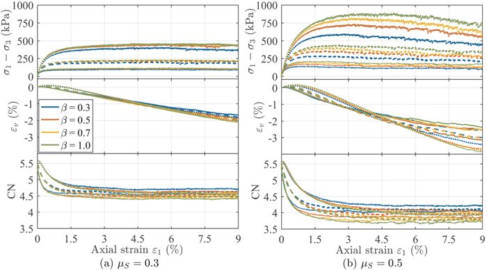
Figure 5. Evolution of the deviator stress, the volumetric strain, and the mechanical coordination number of granular specimens as functions of the axial strain in triaxial compression tests for (a) μS = 0.3, and (b) μS = 0.5, where the solid, dashed, and dotted lines correspond to a confining pressure of 50 kPa, 100 kPa, and 200 kPa, respectively. The results for different β are presented in different colors as indicated in the legend.
Download figure:
Standard image High-resolution imageIn addition, some conspicuous features of the effect of μS and β can be observed under each confining pressure:
- 1.The deviator stress as well as its peak value and the corresponding axial strain at the peak state all increase with μS and β.
- 2.The maximum compaction in the volumetric strain and the corresponding axial strain increase with μS and β.
- 3.The value of CN at the dilation stage decreases as μS or β increases.
The above findings indicate that higher friction resistance can improve the robustness of the contact force network and require more effort to disrupt its structure.
The shape parameter β seems to play a smaller role than the sliding friction coefficient μS does, especially for the cases of μS = 0.3. Figure 6(a) compares the peak stress variables and the corresponding failure envelopes in the I1– plane for different μS with various β. Generally, a higher friction angle ϕ can be achieved with a larger μS or β, which is physically expected. However, as shown in Figure 6(a) and Table 1, the effect of β on the friction angle ϕ declines when β becomes larger, and the maximum achievable friction angle is limited by the value of μS, e.g., ∼32° for μS = 0.3. This implies that the shear strength of a granular assembly is strongly controlled by the sliding frictional resistance between components. Once particles start sliding relative to each other, the rotational resistance, regardless of how large it is, cannot stop this process, and the shear strength will be weakened, resulting in the strain-softening behavior. As shown in Figure 5, this strain-softening behavior is more pronounced with larger μS, in agreement with previous simulations (e.g., Göncü & Luding 2013).
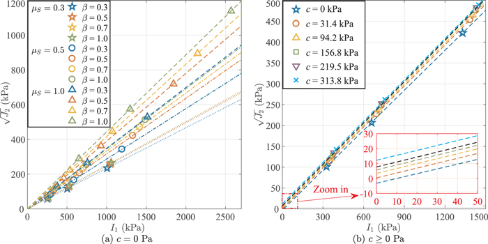
Figure 6. Peak stress variables of triaxial compression tests and corresponding failure envelopes plotted in I1– plane for (a) c = 0 Pa (simulations 1 to 12), where the dotted, dash–dotted, and dashed lines correspond to μS of 0.3, 0.5, and 1.0, and the results for different β are presented in different colors as indicated in the legend; and (b) c ≥ 0 Pa (simulations 6 and 13 to 17), in which the inset gives a closer view of the origin, showing the changes in the intercept for each curve. Linear least-squares fitting is applied to draw the failure envelopes.
Download figure:
Standard image High-resolution image3.3.2. Effect of the Interparticle Cohesive Tensile Strength c
A series of triaxial compression tests were performed with μS = 0.5, β = 0.5, and the interparticle cohesive tensile strength c varying from 0 to 313.8 kPa, corresponding to simulations 6 and 13 to 17 in Table 1. Figure 6(b) presents the failure envelopes at the peak state in the I1– plane of these tests. An apparent macroscopic cohesive strength C (i.e., the intercept) is observed for nonzero c, and grows with c. The friction angle ϕ (i.e., the slope) is essentially independent of c, which is consistent with the findings in previous simulations (e.g., Modenese et al. 2012; Jiang et al. 2013). Combined with Figure 6(a), the results indicate that the shear strength mainly depends on the sliding friction coefficient, μS, and the interparticle contact area, β, while the cohesive strength primarily depends on the interparticle cohesive tensile strength c (and on β, since it controls the contact area).
The consistency of results from our triaxial compression tests with those from laboratory experiments allows us to extend our SSDEM model to simulate granular materials in other scenarios with confidence. In the following section, this model is applied to study spinning rubble-pile bodies in space. A similar failure analysis procedure is carried out to investigate the material strengths of these bodies (see Section 5).
4. Application: Numerical Modeling of Spinning Rubble Piles
As indicated by previous SSDEM studies on spinning self-gravitating aggregates (e.g., Sánchez & Scheeres 2012, 2016; Zhang et al. 2017), the spin limit of a rubble pile strongly depends on the friction and cohesion parameters of the contact model. However, these studies did not distinguish the contribution of the sliding friction and rotational friction to the material strength, and the action of these parameters has not been fully understood. In this study, we attempt to reveal the mechanisms of these parameters through analyzing rubble-pile structures during spin-up processes from multiple scales.
4.1. Simulation Setup
The granular representations of rubble-pile asteroids with a given shape are constructed using the same procedure as described in Section 3.1. An oblate model with axis ratios α1 of ∼0.9, α2 of ∼1.0, a maximum diameter of ∼1 km, and a bulk density ρB of ∼2.4 g/cc is taken as the rubble-pile sample in this analysis, where α1 = a3/a1, α2 = a2/a1. The axis lengths a1, a2, and a3 are given as the maximum extensions along the principal axes of inertia (from largest to smallest) of the rubble pile. The bulk density of a rubble pile is calculated as ρB = ηBρp, where ηB is the internal packing efficiency (defined in Equation (9)) and ρp is the particle material density. This rubble-pile model consists of ∼18,000 particles, with a −3-index power-law distribution in particle radius ranging from 10 m to 30 m, and ρp of ∼3.3 g/cc.12 The normal stiffness kN and the timestep Δt are set to meet the maximum particle overlap requirement.
During a spin-up simulation, with given SSDEM parameters, the simulated rubble pile evolves under its self-gravity, following a spin-up path, which sets its spin period T to a prescribed value as a function of time t (see the top frame in Figure 7 for an example; only maximum principal-axis rotation is considered in this study, where z is the spin axis). The spin-up procedure is similar to our previous study (see Section 2.3.4 in Zhang et al. 2017, for details). In brief, in the beginning of a simulation, the rubble-pile body is allowed to settle down at a slow spin state Tstart (Tstart = 4 hr is used in this study), and then, the body is linearly spun up from Tstart until global disruption occurs, after which we stop maintaining the spin period of the simulated body and let the body evolve freely under its own gravity.13

Figure 7. Evolution of spin period (T, top frame), axis ratio (α1, upper middle frame), internal packing efficiency (ηB, lower middle frame), and mechanical coordination number (CN, bottom frame) during spin-up processes. The results for different μS and β are denoted in different colors as indicated in the legend. c = 0 Pa for all the cases shown here.
Download figure:
Standard image High-resolution image4.2. Definitions of Multiscale Variables
Considering that the mechanical behaviors of granular materials have different interpretations when analyses are carried out at different scales (Andrade & Tu 2009), variables defined at three different scales are monitored throughout the spin-up process. At the global scale, the shape, characterized by α1 and α2, the internal packing efficiency, ηB, and the mechanical coordination number, CN, are used to capture the global properties of the simulated body. The internal packing efficiency ηB is the fraction of the volume in the internal structure of a rubble pile that is occupied by the constituent particles, which can be measured based on the Voronoi tessellation of this rubble pile (see Section 3.2 in Zhang et al. 2017, for details),

where ri is the radius and Vi is the volume of the Voronoi cell for the ith particle, and Ninternal is the number of particles in the interior of the rubble pile.
The global dynamical behaviors of a granular material depend on the interaction of individual particles at the microscopic scale, which can be captured by the force chain distribution. The contact networks in the simulated rubble pile can be visualized by tracing the normal contact strength, SN, i.e., the total normal contact force divided by the effective contact area, so that the contacts that reach the cohesion limit (i.e., the given value of the interparticle cohesive tensile strength c used in the simulation) are revealed.
Furthermore, to link the properties of the simulated rubble pile with the conventional continuum medium and present the local characteristics at the macroscopic scale, it is also useful to analyze the stress distribution in the rubble pile. The stress analyses are carried out on the scale of representative volume elements (RVEs; see Section 3.3.1 in Zhang et al. 2017, and references therein for details). The size of an RVE is often taken to be about 12 times the radius of the typical particle for stress analyses (Masson & Martinez 2000). We use a tree code to divide the rubble-pile body into several similar-sized sub-assemblies, i.e., RVEs. Each RVE contains 200 to 300 particles. The average stress tensor of a local region, e.g., the jth RVE, in a rubble pile can be assessed by homogenization and averaging methods,
where NRVE is the number of particles in this RVE and VRVE is the total volume of this RVE. The Cauchy stress tensor  for a single particle i is given as the summation of the dyadic product of the branch vector
  that connects the particle center with the contact point and the corresponding contact force
  for the kth contact. Ni,C is the number of contacts for the ith particle. The first invariant of the average stress tensor
  and the second invariant of the deviatoric stress tensor
  for the jth RVE can be determined from the averaged stress tensor
  . Analyzing the distribution of these stress-state variables can help us interpret how the simulated rubble pile responds to the spin-up loads.
4.3. Spin-up Simulation Results
To understand the effect of the SSDEM parameters on the dynamical behaviors and material strengths of rotating rubble piles, multiple spin-up simulations were carried out in this study, as summarized in Table 2.
Table 2. Summary of Simulation Parameters (Second Column to Fifth Column) and the Critical Spin Period (Sixth Column) and Material Strengths (Last Two Columns) of Simulated Rubble Piles in the Spin-up Testsa
| Sim. No. | μS | β | c (Pa) | ρB (g/cc) | Tc (hr) | ϕ (°) | C (Pa) |
|---|---|---|---|---|---|---|---|
| 1.8 | 3.00 | ||||||
| 1 | 0.5 | 0.3 | 0 | 2.4 | 2.60 | 31.7 ± 0.6 | −0.1 ± 0.2 |
| 3.0 | 2.32 | ||||||
| 1.8 | 2.96 | ||||||
| 2 | 0.5 | 0.5 | 0 | 2.4 | 2.56 | 32.9 ± 0.5 | 0.0 ± 0.2 |
| 3.0 | 2.28 | ||||||
| 1.8 | 2.93 | ||||||
| 3 | 0.5 | 0.7 | 0 | 2.4 | 2.54 | 33.7 ± 0.4 | 0.1 ± 0.2 |
| 3.0 | 2.27 | ||||||
| 1.8 | 2.92 | ||||||
| 4 | 1.0 | 0.3 | 0 | 2.4 | 2.53 | 34.2 ± 0.8 | 0.1 ± 0.3 |
| 3.0 | 2.27 | ||||||
| 1.8 | 2.90 | ||||||
| 5 | 1.0 | 0.5 | 0 | 2.4 | 2.51 | 35.2 ± 0.7 | 0.0 ± 0.3 |
| 3.0 | 2.24 | ||||||
| 1.8 | 2.87 | ||||||
| 6 | 1.0 | 0.7 | 0 | 2.4 | 2.49 | 36.1 ± 0.5 | 0.1 ± 0.2 |
| 3.0 | 2.22 | ||||||
| 1.8 | 2.94 | ||||||
| 7 | 0.5 | 0.5 | 100 | 2.4 | 2.49 | 33.3 ± 0.6 | 0.8 ± 0.2 |
| 3.0 | 2.23 | ||||||
| 1.8 | 2.71 | ||||||
| 8 | 0.5 | 0.5 | 200 | 2.4 | 2.42 | 33.1 ± 0.2 | 2.1 ± 0.1 |
| 3.0 | 2.20 | ||||||
| 1.8 | 2.59 | ||||||
| 9 | 0.5 | 0.5 | 400 | 2.4 | 2.34 | 33.1 ± 0.9 | 5.2 ± 0.3 |
| 3.0 | 2.13 | ||||||
| 1.8 | 2.38 | ||||||
| 10 | 0.5 | 0.5 | 800 | 2.4 | 2.20 | 32.7 ± 0.4 | 12.7 ± 0.1 |
| 3.0 | 2.04 | ||||||
| 1.8 | 1.95 | ||||||
| 11 | 0.5 | 0.5 | 1600 | 2.4 | 1.97 | 32.0 ± 1.3 | 28.7 ± 0.5 |
| 3.0 | 1.88 | ||||||
Note.
aThe values of ϕ and C are reported within their 90% confidence intervals.Download table as: ASCIITypeset image
4.3.1. Effect of Interparticle Friction Parameters: μS and β
Figure 7 shows the evolution of the state variables of the simulated body during the spin-up process for different sets of parameters, μS and β, with c = 0 Pa. The top left panel of the Figure 12 animation presents the spin-up and disruption process in the case of μS = 0.5, β = 0.5, and c = 0 Pa. As expected, an increase in the sliding friction or rotational friction can postpone the initiation of failure. When the body has been spun up past its failure limit, its shape becomes more oblate, and the packing efficiency and coordination number gradually decrease. The evolution of these state variables exhibits similar failure behaviors, regardless of the value of μS or β. The finding that the failure mode does not show strong dependencies on the friction parameters is in agreement with the analytical theory by Hirabayashi (2015). The simulations of Sánchez & Scheeres (2016), using a different SSDEM code, show a contrary result, namely that different friction angles lead to different disruption patterns. A plausible explanation for this is that they achieved different friction angles by turning off the rolling friction and the sliding friction separately, which changes the intrinsic properties of the contact network, and so the dynamical characteristics are different. In reality, neither the rolling friction nor the sliding friction is negligible for natural granular materials. Therefore, the failure mode should not be strongly affected by the frictional strength if both kinds of friction are turned on.
We take the case of μS = 0.5 and β = 0.5 as a representation to detail the characteristics of a cohesionless rubble pile during the spin-up process. Figure 8 illustrates the distribution of the stress-state variables and the contact strength networks over a cross-section of the simulated rubble pile at the slow spin state (T = 4.00 hr), the moderate spin state (T = 2.90 hr), and the critical spin state (T = 2.56 hr, which is the critical spin period for this model; see Section 5 for details about how to determine the critical spin limit of a rubble-pile body using SSDEM). Figure 9 compares the distributions of contact orientations in the rubble pile at different spin states. As would be expected for this random configuration, the distributions of contact force orientations are uniform at slow spin (see the areas encompassed by the blue curves in Figure 9). Since the centrifugal forces become larger as the spin rate increases, the force chains parallel to the x–y plane gradually break or rearrange themselves in other directions, leading to an asymmetric distribution of contact orientations (Figures 8(g)–(i); also see the areas encompassed by the red and orange curves in Figure 9). As shown in the first row of Figure 8, increasing the centrifugal forces also diminishes the central pressure for this body. Meanwhile, given that the forces along the vertical direction caused by gravity remain constant, the body experiences larger shear stresses as the spin rate increases (second row of Figure 8), and the strong force chains gradually align parallel to the rotation axis (bottom row of Figure 8).
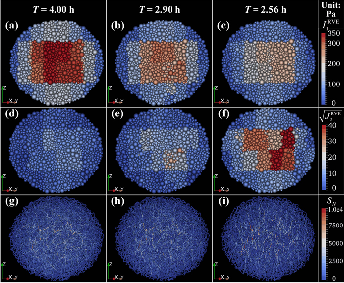
Figure 8. Simulation case of μS = 0.5, β = 0.5, and c = 0 Pa: distributions of stress-state variables, IRVE1 (first row),  (second row), and the contact strength networks (bottom row), over a cross-section parallel to the maximum moment of inertia axis at different spin periods for the simulated rubble pile. The patches shown represent the RVEs in these cross-sections. Due to the heterogeneity arising from the particle arrangement and the RVE division, the distribution of the stress-state variables cannot be perfectly symmetrical.
Download figure:
Standard image High-resolution image
Figure 9. Simulation case of μS = 0.5, β = 0.5, and c = 0 Pa: distributions of contact orientations for different spin periods (denoted by different colors), where z is the spin axis and the x–y plane is parallel to the equatorial plane.
Download figure:
Standard image High-resolution imageAlthough the evolution of the state variables follows the same trend and the failure mode is independent of μS or β, the failure spin of the rubble pile shows clear dependencies on the interparticle friction parameters. That is, the rubble pile can be stable at a higher spin rate as μS or β increase (see Table 2 for a summary of the critical spin periods). However, the effect of β is less significant than that of μS. When cohesion is not included, the shear failure of a rubble-pile structure is caused by microscale sliding, rolling, and twisting between particles in contact. The friction coefficient μS dominates the sliding resistance, while the shape parameter β dominates the rolling and twisting resistance in SSDEM simulations. Figure 10 shows the distributions of the orientations for the sliding/rolling/twisting contacts at the critical spin state for the case of μS = 0.5 and β = 0.5 (other cases show similar results). The sliding/rolling/twisting contact is defined as the contact mode for which the tangential force/rolling torque/twisting torque exceeds the critical value, μSFN/MR,max/MT,max. As seen in Figure 10, the number of sliding contacts is much larger than that of the rolling or twisting contacts at the critical spin state. This implies that at the microscale of a spinning rubble pile, particle rearrangements are mainly caused by sliding movements between particles in contact, i.e., sliding rearrangement is the preferred mode of particle-level deformation. Therefore, the friction coefficient μS has a much greater impact on the structural stability of rubble piles. Our study reveals the complexity and importance of the interparticle contact mode and friction parameters in controlling the strength and deformation mode of a granular assembly. Furthermore, it is interesting to note that the distributions of the three contact modes have different preferred directions in the y–z and z–x plane. For example, since the mid-latitude regions are subject to the highest slope for such a shape, as revealed by Harris et al. (2009), sliding failure is most likely to develop in these regions (see the areas compassed by the blue curves in Figure 10).

Figure 10. Simulation case of μS = 0.5, β = 0.5, and c = 0 Pa: distributions of orientations for sliding/rolling/twisting contacts (denoted by different colors) at the critical spin period of 2.56 hr.
Download figure:
Standard image High-resolution image4.3.2. Effect of Interparticle Cohesive Tensile Strength c
Since the cohesive strength of the interstitial regolith arising from van der Waals forces could range from hundreds of pascals to thousands of pascals in asteroids (Sánchez & Scheeres 2014; Gundlach & Blum 2015), the interparticle cohesive tensile strength c was selected to be 100 to 1600 Pa for the cohesive SSDEM simulations presented in this section, in which μS and β were both set to 0.5. As shown in Figure 11, the evolution of the rubble pile progresses in different manners with changes in c. The existence of cohesion can improve the strength of the contact force network by increasing the coordination number and the packing efficiency. As c increases, the rubble-pile structure can maintain its shape and internal packing efficiency at a higher spin rate, and the amount of deformation that appears before disruption decreases, followed by a more abrupt disruption process.

Figure 11. Same as Figure 7, but for different interparticle cohesive tensile strength c, as indicated in the legend. μS = 0.5 and β = 0.5 for all the cases shown here.
Download figure:
Standard image High-resolution imageIn addition, the style of fragmentation during the disruption process also shows a strong dependence on c, as shown in Figure 12 (also see the animation of Figure 12 for the spin-up and disruption processes with different c). Recall that the spin period of the simulated body is strictly constrained to the spin-up path until α1 is reduced to half of its initial value, so the body is continuously subject to the spin-up loading even after its structure fails. Normally, for kilometer-size asteroids, the timescale of the YORP loading process exceeds 104 years (Rubincam 2000), which is much longer than the dynamical time needed for a rubble pile to settle down in the absence of external forces. Therefore, in reality, the low-cohesion rubble pile is more likely to shed some surface materials or slightly deform to offset the extra spin, rather than completely break up. However, for the high-cohesion cases, since the deformation of the rubble pile before disruption is inhibited, the disaggregation behaviors of the high-cohesion rubble piles observed in the spin-up tests could represent the failure behaviors of real cohesive rubble-pile asteroids. Taking the cases of c = 0 Pa and c = 800 Pa as examples, we carried out two other runs without continuous rotational acceleration. In both cases, the body is spun up to a spin period below its critical value and is forced to stay at this spin period until α1 is reduced by 0.1, after which the body is set to be free of external forcing. Figure 13 presents the outcomes of these two simulations, and the animation of Figure 13 records the evolution processes. As can be seen in the animation of Figure 13, instead of continuous deformation as observed previously (see the top left panel in the animation of Figure 12), landslides and mass shedding are the main failure features for the cohesionless body, while the failure behavior for the cohesive case is almost the same as that shown in the continuous spin-up test (see the bottom left panel in the animation of Figure 12). The distinguishing failure behaviors of the cohesive body could be used to reveal the level of cohesion in a disintegrating asteroid from observations.
Figure 12. Images after the simulated bodies fail for different c. The spin period T of each body at the shown moment is given in the top right corner of each image, and all particles are colored by their translational speed as indicated in the color bars (note that the objects started as oblate shapes in all cases; the corresponding animation shows the full evolution for all six panels. The spin periods of the six simulated bodies start at T = 2.60 hr and end at 2.42 hr, 2.38 hr, 2.34 hr, 2.26 hr, 2.14 hr, and 1.90 hr).
(An animation of this figure is available.)
Download figure:
Video Standard image High-resolution imageFigure 13. Same as Figure 12, but for the scenarios without continuous rotational acceleration (the corresponding animation shows the full evolution for both panels. The spin periods of the two simulated bodies start at T = 2.52 hr and 2.19 hr). Since the body is set to be free of external forcing after disruption occurs, its spin period can adjust rapidly to maintain conservation of total angular momentum, as shown in the case of c = 800 Pa.
(An animation of this figure is available.)
Download figure:
Video Standard image High-resolution imageAs shown in Figure 12 (also see the bottom panels in the animation of Figure 12), when the cohesion is high enough, i.e., the cases of c = 800 and c = 1600 Pa, the rubble pile can directly split into multiple distinct fragments consisting of many particles. For this reason, the value of CN after global disruption in the high-cohesion cases can stay at a moderate constant value (see the bottom frame in Figure 11). Figure 14 shows the cumulative mass distributions of the fragments produced in the rotational fission events for different c. The size distribution of the resulting fragments depends on the cohesive forces that bond particles together. When cohesion is low, the rubble pile will disrupt into individual particles; however, when cohesion is high enough, the rubble pile will disaggregate into similar-size fragments. The disaggregating behaviors of cohesive rubble piles could be a plausible mechanism to form asteroid pairs (Pravec et al. 2010). The resulting fragments escape from each other at speeds on the order of ∼0.5 m s−1, close to the mean pair-wise sky-plane velocity dispersion between fragments of the disintegrating asteroid P/2013 R3 (i.e., 0.33 ± 0.03 m s−1; Jewitt et al. 2017). The properties of the fragments (e.g., size distribution, velocity dispersion) in the high-cohesion cases show many similarities to the observations of P/2013 R3, indicating that this asteroid may possess relatively high cohesion in its structure and experience rotational fission in a manner similar to the high-cohesion cases.

Figure 14. Cumulative fragment mass distributions after global disruption for different c in the continuous spin-up scenarios. The crimson curve (named "Particles") and the black curve reflect the cumulative mass distribution of constituent particles in the rubble-pile model and the major components of asteroid P/2013 R3 (i.e., A1, A2, B1, B2, C1, and C2; for which the estimated mass me = 4/3ρBπre3, where ρB = 1.0 g/cc and re is the minimum radius of the equal-area circle listed in Table 4 of Jewitt et al. 2017).
Download figure:
Standard image High-resolution imageThe effect of cohesion, whereby deformation is diminished prior to disruption and the component size of the fissioned material is increased, was also observed in the numerical study of Sánchez & Scheeres (2016) using a different SSDEM code. However, unlike our high-cohesion cases, where the body is observed to axisymmetrically disaggregate into similar-size fragments, their simulations generally show that the rubble pile is disrupted by non-axisymmetric deformation and partial fission, even in the spherical case (see Table B.3 in Sánchez & Scheeres 2016). This behavior is expected when the simulated rubble pile possesses a non-uniform particle arrangement in the rotation axis direction, which leads to a non-uniform distribution of structural strength, but not when the body is axisymmetric (Holsapple 2008). The observed difference, therefore, may be due to the axial non-uniformity of the particle arrangement in the rubble-pile models used by Sánchez & Scheeres (2016). In addition, the discrepancy in the spin-up path and the numerical model between our study and theirs may also account for this difference.
Figure 15 shows the distributions of the stress-state variables and the contact strength networks over a cross-section of the simulated body with c = 800 Pa, at the slow spin state (T = 4.00 hr), the critical spin state for the cohesionless case (T = 2.56 hr), and the critical spin state for itself (T = 2.20 hr). The contact force networks consist of a significant number of cohesive force chains (i.e., the chains with SN < 0), even in the slow spin state, which can slow down the breakage of force chains. As the spin rate is increased, some of the force chains, especially those parallel to the equatorial plane, reach the cohesion extremum, i.e., 800 Pa in magnitude for this case, implying that the corresponding particles are barely in contact with each other, and the connection could break as the spin-up process continues. As shown in the bottom frame of Figure 11, the amount of contacts that are lost before disruption dramatically decreases as c increases. Thus, failure in this high-cohesion body is likely to be stimulated when a sufficient number of cohesive force chains reach the cohesion extremum and break all together within a short time span.

Figure 15. Same as Figure 8, but for the case of μS = 0.5, β = 0.5, and c = 800 Pa.
Download figure:
Standard image High-resolution imageComparing the case for T = 2.56 hr in Figure 15 with that in Figure 8, it is evident that higher cohesive strength can impose higher pressure and ease the shear stresses in the interior. Remarkably, the stress states of some surface regions transform from a compressive mode into a tensile mode as the spin rate increases (Figure 15(c)). The failure envelope analyses in Section 5.2 indicate that the failure point for this body occurs in the second quadrant in the  plane (see Figure 16). Therefore, the damage of the surface structure is mainly caused by tensile failure rather than shear failure in the high-cohesion case. As observed in the bottom panels in the animation of Figure 12, the fracture of the surface region can propagate into the interior region and stimulate the disaggregation of the whole body.
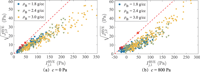
Figure 16.
 vs.
vs.  for each RVE at the critical spin state for (a) c = 0 Pa and (b) c = 800 Pa, where μS = 0.5 and β = 0.5 in both cases. The results of different densities are shown in different colors as indicated in the legend. The failure point for each density is highlighted by a red symbol. Linear least-squares fitting is applied to draw the failure envelopes (i.e., the dashed lines).
Download figure:
Standard image High-resolution image5. Critical Spin Limits and Material Strengths of Rubble Piles
The study of Zhang et al. (2017) showed that the failure condition of a cohesionless rubble pile subject to rotational acceleration in SSDEM simulations can give information about the shear strength of the body. By testing the creep stability of the simulated rubble pile at different spin periods, they obtained the critical spin state at which the rubble pile can be just geostatically stable with its original shape without further creep deformation. The corresponding spin rate is the critical spin rate for the tested body, and the friction angle can be derived by substituting the stress state of the tested body at this critical spin state into the failure criterion.
In this study, we use the same procedure to determine the critical spin state and the critical spin period Tc for simulated rubble piles. Note that as there are two unknown material strength parameters, ϕ and C, for a cohesive rubble pile, the original method in Zhang et al. (2017) designed for the cohesionless case cannot be directly employed. Here, based on the mechanical characteristics of granular materials, we propose an improved method to derive the macroscopic friction and cohesion properties of the simulated rubble piles.
5.1. Determination of the Friction Angle ϕ
According to the Drucker–Prager failure criterion, the failure condition of a granular assembly depends on both the shear stress and the pressures that act on it, so that the failure envelope can be drawn at several failure points under different confining pressures, as shown in the triaxial compression tests (e.g., see Figure 6). Normally, when compared to the material strength of a rubble-pile asteroid, the surface pressure, e.g., caused by the solar radiation pressure, is negligible, and the boundary of this body can be treated to be stress-free, which means the confining pressures are all zero. Therefore, instead of varying the surface pressure as done in the triaxial compression tests, we achieve various pressure conditions by changing the bulk density of the simulated rubble pile. For each SSDEM parameter set, (μS, β, and c), in addition to the nominal runs with the bulk density of 2.4 g/cc as used in Section 4, two other simulations with bulk densities of 1.8 g/cc and 3.0 g/cc were carried out to support the failure envelope analyses.
Since the stress state will vary throughout a rubble-pile structure (see Figure 8 for examples), the next step is to determine the failure stress state for each bulk density case. Previous studies show that the starting point of failure in a rubble pile always occurs locally in a region that is subject to the highest shear-pressure ratio (e.g., Hirabayashi 2015; Zhang et al. 2017). The RVEs can serve as the smallest element for the stress analyses. To measure how close an RVE is to its structural failure point, we introduce a new variable, the stress ratio λ, which for the jth RVE is given by

where C and s are the strength parameters used in the Drucker–Prager failure criterion (see Section 3.2). If this stress ratio exceeds 1, the jth RVE should experience plastic deformation. When the material is cohesionless, λRVEj is proportional to the ratio of  to
to  . This implies that the part in a cohesionless rubble pile most sensitive to failure should possess the highest
  .
.
Figure 16(a) shows the stress-state variable distribution of a rubble pile's RVEs at the critical spin state in the I1– plane for the case of μS = 0.5, β = 0.5, and c = 0 Pa. It is evident that the shear stress and the pressure at the failure state of this rubble pile increase in proportion to the bulk density. The failure point is identified as the one that has the highest
  for each bulk density case, i.e., the red symbols in Figure 16(a). Then, the values of ϕ and C can be determined from the best-fit failure envelope, i.e., the dashed line in Figure 16(a). We use this method to derive the strength parameters for all cohesionless cases. As shown in Table 2 (simulations 1 to 6), a higher friction angle ϕ can be achieved with a larger μS or β. Since there is no apparent cohesion in the material, the values of C are very close to zero. Furthermore, it is interesting to note that there are significant differences between the friction angle obtained from the spin-up tests (see Table 2) and that in the triaxial tests (see Table 1), indicating the high sensitivity of the properties of a granular material to the loading scenario and the particle arrangement.
5.2. Determination of the Macroscopic Cohesive Strength C
When cohesion is present, the search for the failure point becomes complex due to the uncertainties of both C and s in Equation (11). Our triaxial simulation results showed that the friction angle is essentially independent of the interparticle cohesive tensile strength c. For simulations with the same μS and β, it is therefore proper to assume that their failure envelopes have the same slope. By translating the failure envelope obtained from the corresponding cohesionless case up and down, the failure point for each simulation can be identified as the one that has the largest intercept in the I1– plane.
Figure 16(b) shows the stress-state variable distribution of a rubble pile at the critical spin state for the simulation case of μS = 0.5, β = 0.5, and c = 800 Pa. The failure points determined using the approach introduced above for each bulk density case are highlighted by red symbols. The failure envelope for this cohesive case is then established through a linear least-squares procedure, which provides the friction angle ϕ and the cohesion C. Using this method, the values of ϕ and C were derived for all cohesive rubble piles in our simulations, as presented in Table 2. The small differences in estimates of the friction angle shown in the results once again confirm the independence between c and ϕ. Thus, as a practical matter, to save the effort of conducting two more spin-up tests, the value of C can be directly estimated from one failure point by assuming the friction angle is the same as the cohesionless case.
As shown in Table 2 (simulations 7 to 11), the macroscopic cohesive strength C is on the order of one percent of the interparticle cohesive tensile strength c and displays a nonlinear correlation with c. This is because a higher c can increase the number of cohesive connections and enhance the efficiency of cohesion, as discussed in Section 4.3.2. Our high-cohesion cases show that C of ∼30 Pa is enough to stimulate the disaggregating behavior of rubble-pile asteroids. Therefore, the observed active asteroid P/2013 P3 may possess cohesion close to or higher than this value. This argument is consistent with the velocity dispersion between fragments from observations, which indicates an effective cohesive strength ∼50–100 Pa (Jewitt et al. 2017).
5.3. Stress Ratio Distribution and Failure Mode
Figure 17 plots the distributions of the stress ratios over the internal structure for the cases of c = 0 Pa and c = 800 Pa, with μS = 0.5, β = 0.5. The corresponding values of ϕ and C listed in Table 2 are used to calculate the stress ratios for each RVE. It is evident that increases in cohesion can postpone the onset of failure. As shown in Figure 17, the rubble piles are well below the failure condition at the slow spin state, and the stress ratios generally grow with the spin rate. The initial failure occurs at the surface near the equatorial region in both cases, but different failure behaviors are observed. A surface shedding-failure mode caused by shear failure of particles resting on the surface is confirmed for the cohesionless case (see the left panel in the animation of Figure 13), while a surface tensile-failure mode is identified for c = 800 Pa (see the right panel in the animation of Figure 13 and the last paragraph in Section 4.3.2). Our study indicates that in addition to the distribution of stress ratios, information on pressure states is also needed to properly predict the failure mode.

Figure 17. Distributions of stress ratios, λRVE, over a cross-section parallel to the maximum moment of inertia axis at different spin periods for the simulated rubble piles with c = 0 Pa (first row) and c = 800 Pa (second row), where μS = 0.5 and β = 0.5.
Download figure:
Standard image High-resolution image6. Comparison between SSDEM Analyses and Continuum Theory
Several analytical methods based on continuum theory have been developed to reveal the failure mechanisms of spinning rubble-pile bodies. According to the choice of stress solutions to the problem, these methods fall into two categories, i.e., the volume-averaging method (e.g., Holsapple 2004, 2007; Sharma 2013), and the method for analyzing the elastic stress distribution (e.g., Dobrovolskis 1982; Hirabayashi 2015). Based on the classical upper-bound approach of plastic limit analysis, Holsapple (2008) showed that the global-volume-averaging method can give an upper-bound condition on the critical spin rate where the structure would fail globally. The second method can determine the distribution of stress-state variables in a body and characterize the region most sensitive to failure (Hirabayashi et al. 2015). In this section, we combine these analytical theories to reveal the implications of our numerical results. The simulation cases with bulk density 2.4 g/cc are taken as representative cases for this topic.
6.1. Stress Distribution
The complete elastic solution of a gravitational spinning ellipsoid in equilibrium can be obtained by solving the elastic equations (where Hooke's law is used to describe the constitutive relation). Dobrovolskis (1982) presented the derivation in detail. Hirabayashi (2015) substituted the equilibrium stress solution into the Drucker–Prager failure criterion to analyze the failure condition and mode of a cohesive spherical body. Using a similar approach, we carry out stress analyses for a 1-km-diameter oblate body with an axis ratio α1 = 0.9 at the failure spin for the cases with μS = 0.5, β = 0.5, and c = 0 Pa and μS = 0.5, β = 0.5, and c = 800 Pa (corresponding to C = 12.7 Pa), as shown in Figure 18. The quantity  is the spin rate normalized by
  , where G is the gravitational constant. In both cases, the central region is subject to the highest pressure and the largest shear stress, and as the spin rate increases, the pressure decreases while the shear stress increases. The distribution characteristics of the stress field and the response to rotational acceleration of our simulation results are all consistent with the analytical solutions (e.g., see Figures 8 and 15). The magnitude of the pressure and shear stress field in the cohesionless case even shows quantitative consistency. For example, as shown in Figures 8(c) and (f), the maximum values of
  and
and  appear near the center, which are larger than 200 Pa and 40 Pa at the failure state for the simulated body, respectively. Similar phenomena are also shown in the results of the elastic theory (i.e., Figure 18).

Figure 18. Distributions of I1 (first row),  (second row), and the stress ratio λ (bottom row) over the cross-section along the x and z axes for an oblate body with α1 = 0.9. The left-hand and right-hand columns describe the stress state for C = 0 Pa,
  (i.e., T = 2.56 hr), and C = 12.7 Pa,
  (i.e., T = 2.20 hr), respectively. The elastic analyses are used to draw this distribution. A friction angle of 33.0° and Poisson's ratio of 0.25 are used for both cases.
Download figure:
Standard image High-resolution imageAs characterized by the stress ratio λ (bottom row in Figure 18), the equatorial surface is the most sensitive part when the rubble-pile structure yields for C = 0 Pa, in agreement with our numerical results for c = 0 Pa (see Figure 17), while the central region is subject to the highest stress ratio in the high-cohesion case. This phenomenon was discussed in the analytical study of Hirabayashi (2015), where he found that for a homogeneous, cohesive body, the region subject to the highest relative shear stress migrates from the equatorial surface to the central region as the dimensionless spin rate increases to near 1. The inconsistency between our numerical results and Hirabayashi's theory in the high-cohesion case may come from the differences between the cohesion mechanism in the discrete element modeling and that in the continuum method. The cohesive strength can be completely controlled by a specific variable in continuum analyses (e.g., C in the Drucker–Prager failure criterion), while the distribution of the macroscopic cohesive strength cannot be perfectly uniform in a discrete element model even for a constant c due to heterogeneity of radial particle arrangements. As revealed by Zhang et al. (2017), the local packing efficiency and coordination number for the surface particles is much lower than that for the interior particles. Therefore, the local macroscopic cohesive strength is lower in the surface region for a rubble-pile model, resulting in a weaker surface shell. As a result, surface tensile failure is observed for high-cohesion bodies in the SSDEM simulations.
Overall, our simulation results show good consistency with the results of elastic theory in the cohesionless case, while the elastic theory fails to explain our findings for the cohesive model. In fact, in the course of solving the elastic equations, no information on the cohesion is taken into account. The value of C only affects the calculation of the stress ratio, and the distributions of the pressure and the shear stress are irrelevant to the cohesive strength. This treatment in the analytical method is therefore incorrect. As highlighted in our study (Section 4.3.2; also see Figure 15), the existence of cohesion changes the topology of the force network, where higher cohesive strength can impose higher pressure and ease the shear stress in the interior of a rubble pile. Furthermore, the usage of elastic theory implicitly requires an initial globally stress-free state, which is an unrealistic assumption for natural granular mediums in space (Holsapple & Michel 2006). Meanwhile, the stress-strain relation for a granular assembly is nonlinear generally (see Figure 5 for examples). Therefore, the actual stress distribution in a rubble pile (especially when cohesion is present) could be quite different from the results of elastic theory. Special care should be taken when using the elastic theory to predict the behavior of a cohesive rubble-pile body.
6.2. Spin Limits
Since the state of a body when global failure will occur is independent of the loading history, the global-volume-averaging method can give an upper-bound condition on the critical spin rate (Holsapple 2008). Figure 19 shows the scaled critical spin rate for our 11 simulation cases with μS = 0.5 and β = 0.5 listed in Table 2 compared to the theoretical upper spin limits for various C derived by Holsapple (2007). The spin limits of the cohesionless cases are well described by the continuum theory, while the cases with nonzero c plot above the theoretical upper spin limit. For example, the model with c = 200 Pa, whose macroscopic cohesive strength C is determined to be 2.1 ± 0.1 Pa, can maintain its original shape at a spin rate higher than the theoretical spin limit derived for C = 5 Pa. This implies that our method for determining the material strengths of simulated rubble piles may underestimate the macroscopic cohesion. In fact, as discussed in Section 6.1, the surface region in a simulated rubble pile is naturally weaker than its interior. Given that the surface of the cohesive body fails first and the macroscopic cohesion is estimated according to the stress in this region, the obtained value of C is expected to be lower than the averaged cohesive strength of the whole body as used in the continuum theory.

Figure 19. Critical spin rates of self-gravitating bodies. The solid curves denote the theoretical upper spin limits derived for an oblate body (α1 = 0.9, a = 1 km, ρB = 2.4 g/cc) with different C as indicated in the legend, and the symbols represent the results of our simulations for bulk density 2.4 g/cc, which are labeled with the simulation number; the error bars indicate the 90% confidence intervals in the measurement of friction angles (see Table 2). For the results of simulations with c > 0 Pa, the corresponding measured C value for each is shown next to the simulation numbers.
Download figure:
Standard image High-resolution image
7. Conclusions and Perspectives
This paper explored the effect of shear and cohesive strengths on the mechanical behaviors of self-gravitating rubble piles subject to rotational acceleration, based on SSDEM simulations. A comprehensive contact model incorporating the translational and rotational friction and cohesive interactions was developed for this purpose, whose performance was validated by a series of numerical triaxial compression tests. In this model, the interparticle frictional strength imposed by sliding resistance and rotational resistance and the interparticle cohesive strength are controlled by three independent parameters, μS, β, and c, respectively. We can therefore test the effect of different strengths separately. Spin-up tests on an oblate rubble-pile model show that
- 1.an increase in the sliding friction or rotational friction or cohesion can keep the rubble pile stable at a higher spin rate;
- 2.when cohesion is not included, the shear failure of the rubble pile is dominated by microscale sliding between particles in contact, and the failure behaviors are independent of the friction parameters, μS and β, where landslides and mass shedding are the main failure features;
- 3.the failure behaviors show a strong dependence on the value of the cohesion parameter c, e.g., as c increases, the amount of deformation that appears before disruption decreases, the disruption process becomes more abrupt, and the component sizes of the fragments resulting from the disruption event increase; and
- 4.when c is high enough, the rubble pile can disaggregate into similar-size fragments, which could be a plausible mechanism to form asteroid pairs and disintegrating asteroids.
The similarities between our high-cohesion result and the observation of active asteroids (e.g., asteroid P/2013 R3) implies that our SSDEM method has great potential in predicting the behaviors of cohesive rubble-pile asteroids. Given that the outcomes should depend on the initial conditions (e.g., the original body size, shape, bulk density, and macroscopic heterogeneity), which we did not explore specifically in this study, it is expected that by conducting spin-up simulations with various conditions, our model could give reasonably accurate constraints on the physical properties of the precursor body for this type of object.
By analyzing the stress state of a simulated rubble pile at failure and fitting the Drucker–Prager failure envelop, we proposed a new method for assessing the macroscopic material strengths (i.e., the friction angle ϕ and the macroscopic cohesion C) of the body. The results show that
- 1.increases in μS or β lead to a larger friction angle;
- 2.the friction angle is essentially independent of c; and
- 3.apparent macroscopic cohesion can be detected when c is nonzero, and the interactive cohesive strength between boulders in contact on an asteroid could be about 100 times the macroscopic material cohesive strength of this asteroid.
The relation between the microscopic interparticle interactions and the macroscopic material properties found in this study could be useful in interpreting the regolith grains and boulders distribution data returned by ongoing or future space missions and linking this information with the body's material strength parameters.
Furthermore, the quantitative analyses on the macroscopic strength parameters offer us the opportunity to make comparisons with continuum theory. We found that the failure region and stress distribution predicted by the elastic theory and the spin limit calculated by the global-volume-averaging method show good consistency with our simulation results in the cohesionless case, while the continuum theory fails to explain our findings for the cohesive model. The differences partly come from the heterogeneous distribution of cohesion in our rubble-pile models and are partly due to an inappropriate assumption in the analytical method, namely leaving the cohesion out of the stress calculation. We conclude that special care should be taken when using the continuum theory to predict the behaviors of a cohesive rubble-pile body.
This work was supported in part by NASA grant NNX15AH90G awarded by the Solar System Workings program. Simulations were carried out at the University of Maryland on the yorp cluster administered by the Department of Astronomy and the deepthought and deepthought2 supercomputing clusters administered by the Division of Informational Technology. Y.Z. acknowledges support from the National Natural Science Foundation of China (NO. 11572166). O.B. acknowledges the support of his time on this effort by the NASA Double Asteroid Redirection Test (DART). P.M. and S.R.S. acknowledge support from the French space agency CNES (OSIRIS-REx/BCU62 and Hayabusa2/BCU66), the European Space Agency, as well as Academies of Excellence: Complex systems and Space, environment, risk, and resilience, part of the IDEX JEDI of the Université Côte d'Azur in connexion with its Center for Planetary Origins (C4PO). Visualization support is provided by the POV-Ray ray-tracing package (e.g., Figures 1, 2, 12, 13, and all the animations) and ParaView software (e.g., Figures 8, 15, and 17).
Software: pkdgrav (Richardson et al. 2000; Stadel 2001), Voro++ (http://math.lbl.gov/voro++/), POV-Ray (http://www.povray.org/), ParaView (http://www.paraview.org).
Footnotes
- 7
Since the electrostatic forces are not globally ubiquitous and there is a large range of uncertainties on the strength of asteroids' electric fields (Scheeres et al. 2010), we typically assume that grains of asteroids are uncharged in this study.
- 8
The min() function means that the vector quantity of least magnitude is the one chosen.
- 9
The mathematical model for rolling and twisting torques is the same as the one used for the cohesionless case in Zhang et al. (2017), but with different physical meanings when cohesion is included.
- 10
In rock and soil mechanics, the compressive stress is expressed as a positive value, and the tensile stress is expressed as a negative value, and so is the strain. We follow this convention in the expression of stress and strain variables.
- 11
A granular specimen is considered macroscopically homogeneous if the distribution of particle sizes and their contact orientations is uniform (see Figure 3 for an example). Generally, in laboratory experiments, a real sand sample consists of millions of particles, while simulations of comparable particle numbers require very time-consuming computation. The studies of Jiang et al. (2003, 2013, 2015) show that the main behaviors of granular materials can be captured when the macroscopic homogeneity of SSDEM specimens is guaranteed. By these means, a macroscopically homogeneous specimen containing thousands of particles should be sufficient for the purpose of this study.
- 12
We also tested two other cases with a lower resolution (∼5,400 particles) and a higher resolution (∼60,700 particles) and found no qualitative differences in results.
- 13
A global disruption behavior of a simulated rubble pile is diagnosed when α1 is reduced to half of its initial value. In general, since the structure is globally disrupted, the spin period of the body will abruptly increase after we set it free. For example, as shown in Figure 7, the spin period T keeps decreasing (the top frame) until the axis ratio and the packing efficiency drop abruptly (the upper middle and the lower middle frames).