


Abstract
The fundamental collisional process of charge exchange (CX) has been established as a primary source of X-ray emission from the heliosphere, planetary exospheres, and supernova remnants. In this process, X-ray emission results from the capture of an electron by a highly charged ion from a neutral atom or molecule, to form a highly excited, high-charge state ion. As the captured electron cascades down to the lowest energy level, photons are emitted, including X-rays. To provide reliable CX-induced X-ray spectral models to realistically simulate these environments, line ratios and spectra are computed using theoretical CX cross sections obtained with the multi-channel Landau-Zener, atomic-orbital close-coupling, molecular-orbital close-coupling, and classical trajectory Monte Carlo methods for various collisional velocities relevant to astrophysics. X-ray spectra were computed for collisions of bare and H-like C to Al ions with H, He, and H2 with results compared to available experimental data. Using these line ratios, XSPEC models of CX emission in the northeast rim of the Cygnus Loop supernova remnant and the heliosphere are shown as examples with ion velocity dependence.
Export citation and abstract BibTeX RIS
1. Introduction
The process of charge exchange (CX) has been identified as the source, or a contribution to, X-ray emission spectra of various objects within the solar system, such as cometary (Cravens 1997), Martian (Dennerl 2006), and Jovian (Cravens et al. 2003) atmospheres. In addition, CX with heliospheric neutrals contributes a significant fraction to the soft X-ray background (Galeazzi et al. 2014), as well as in star-forming galaxies (Liu et al. 2012; Cumbee et al. 2016), supernova remnants (Katsuda et al. 2011; Cumbee et al. 2014), and galaxy clusters (Lallement 2004). This collision between a hot ion and a neutral target might dominate the observed X-ray emission spectra of any environment in which a hot plasma interacts with a cool neutral gas. During a CX collision, an electron is transferred from the neutral target into an excited energy level of the ion. In order to have a complete model of X-ray emission from various X-ray emitting sources, it is essential to include realistic CX data, including the CX cross sections for possible interactions.
Since the first observations of comet Hyakutake with ROSAT (Lisse et al. 1996), the X-ray emission spectra of over 30 comets have been studied, and it has been shown that the X-ray emission from these comets is primarily due to solar wind charge exchange (SWCX) with cometary neutrals (Cravens 1997; Krasnopolsky et al. 2004; Bodewits et al. 2007; Dennerl 2010; Ewing et al. 2013; Snios et al. 2016). In these cases, a pure CX X-ray model can provide a reasonable fit to cometary spectra.
The SPEX package (Gu et al. 2016) is a useful tool for determining the contribution of CX in an observed spectrum. This package uses CX cross sections available in the literature and determines missing n- and ℓ-resolved cross sections through scaling relations. Gu et al. (2016) were able to fit the spectrum of comet C/2000 WM1 (LINEAR) shown in their Figure 5 reasonably well using the SPEX package, but an improved fit was made when this package was supplemented with MCLZ data from the Kronos database, incorporating the various neutrals available in a cometary coma (Mullen et al. 2017).
Outside of our solar system, such as in starburst galaxies and supernova remnants, a variety of processes might contribute to the observed X-ray emission, and must be considered in models. In these cases, modeling packages can be useful for determining the contribution of each process. XSPEC (Arnaud et al. 1996) is an interactive X-ray spectral fitting program that is used to fit models to observed X-ray spectra. It is command-driven and can be used for any spectrometer. The AtomDB CX model, or ACX package (Smith et al. 2014), is a CX modeling tool available for use in XSPEC. While it does not include realistic CX cross sections, it is very useful for determining if CX has a significant contribution to an observed spectrum. This model simulates CX by calculating the dominant or peak excited level of the ion to which the electron transfers, which depends on the charge of the ion and the ionization potential of the neutral. It then considers a variety of theoretical (or semi-empirical) ℓ-distributions. However, the CX model is independent of ion velocity. Using the ACX package along with a thermal plasma model available in XSPEC, Zhang et al. (2014) fit the XMM-Newton RGS X-ray spectrum of the star-forming galaxy M82. They determined that about  of the X-ray flux from the 6 to 30 Å (0.4–2 keV) band for the RGS is due to CX.
In this paper, a set of velocity-dependent CX X-ray emission models are described, using the most accurate available theoretical approaches, for H-like and He-like C-Si ions colliding with H, He, and H2. Line ratios are prepared using various theoretical cross sections for collision velocities from 200 to 5000 km s−1 via radiative cascade. All cross sections and line ratios can be found in the Kronos database (see Mullen et al. 2017). The X-ray line ratios for each ion colliding with H and He are then applied in XSPEC models of the Cygnus Loop supernova remnant for a range of collisional velocities, along with the appropriate contributions from other processes. An earlier model (for further details see Cumbee et al. 2014) only considered H-like and He-like C, N, and O ions colliding with H for a single collision energy, 1 keV u−1 (435 km s−1), while the model discussed here has been enhanced to include emission from Ne, Mg, Al, and Si ions and considers a fraction of 10% He for eight collision energies.
2. Charge Exchange Cross Sections
In the process of CX, which is relevant to X-ray emission as opposed to more generally, a highly charged ion ( ), with charge state q, collides with a neutral atom or molecule (B), transferring one or more electrons from the "target" into a highly excited state of the ion
  , where k is 1 for single-electron capture (SEC). The electron then transitions to the lowest energy state with a probability determined by the Einstein A coefficient for spontaneous emission, emitting at least one photon γ. To accurately model CX emission spectra, it is essential to include the effects of many ionization stages, q, and donor (neutral target) species, B, for a given element (projectile) A.
For a single-electron system in which a bare ion collides with a target with a single electron (H, for example), SEC occurs. SEC follows the following steps:
Figure 1 shows an example of the X-ray emission spectra resulting from SEC collisions of Si13+ with H, H2, and He with a collision energy of 1 keV u−1. Note that the dominant line is the Kα line at about 1850 eV because the cascade to the n = 2 manifold acts as a funnel from the higher n-levels. While SEC is typically the dominant CX mechanism, in systems with more than one electron, multi-electron processes might occur and can significantly vary the intensities of the Lyβ and higher lines (Ali et al. 2005). In a fully robust model, multi-electron and autoionizing processes should be considered for systems with multiple electrons. In this paper, we will focus on SEC.
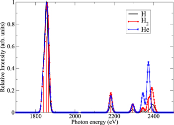
Figure 1. X-ray emission spectra and line ratios (impulses, for H2) of Si12+ following the collision of Si13+ with H, H2, and He at 1 keV u−1 (435 km s−1). MCLZ cross sections are used with a Gaussian resolution of 10 eV.
Download figure:
Standard image High-resolution image2.1. Cross-section Calculations
One of the most important components for producing a realistic CX X-ray emission model is the theoretical cross sections for capture into individual ion quantum states. These state-selective cross sections are known to have sensitive dependencies on the ion velocity. In many cases, the availability and reliability of current CX cross-section data is insufficient to describe the variety of velocities and ion-neutral combinations important in astrophysical systems. Any uncertainties in the state-selective CX cross sections translate to significant uncertainties in the astrophysical models that use them, so it is useful to evaluate theoretical results in light of the very rare measurements available or other theoretical results whenever possible.
In this paper, four methods for producing CX cross sections, relevant at different collision energy ranges, are considered. The quantum-mechanical molecular-orbital close-coupling (QMOCC) approach can in principle be the most accurate method considered here, from the lowest energies to ∼1 keV u−1. The approach presented here considers the CX system as a multi-electron, two-Coulomb-center problem for incident ions. Calculations are performed in two steps. First, the molecular orbitals, energies, and coupling matrix elements are calculated, and then the coupled equations are solved as a quasi-molecular system. The one caveat with QMOCC calculations is dealing with the electronic structure calculations. More details are discussed in Nolte et al. (2012).
The atomic-orbital close-coupling (AOCC) method for the description of ion-atom collision processes is discussed in detail in Fritsch & Lin (1991). This method is relevant from intermediate (∼100 eV u−1) to high (∼10 MeV u−1) energies. For a one-electron two-center collision system, the total electron scattering wave function is expanded over traveling atomic orbitals, which are centered on the target and/or projectile, as well as possibly within the 2-center continuum.
For higher velocities (∼5 keV u−1 to ∼10 MeV u−1), we can consider the classical trajectory Monte Carlo (CTMC) method. This method simulates collisions between ions and atoms by following the trajectories of all particles sampled from an initial ensemble of electron orbits selected in such a manner as to mimic the initial quantum-mechanical momentum space distribution. The motion of the particles is followed by an iterative solution of Hamilton's equations. For bare ion collisions with H, Coulomb potentials are considered, but for multi-electron systems, a model potential is used. After the heavy particles pass through their distance of closest approach and move to an asymptotic distance, the electronic binding energies with respect to each ionic center are calculated to determine what, if any, reaction has occurred, such as excitation, ionization, or charge transfer. The final state in a capture event is determined based on this binding energy and established methods of assigning quantum states to corresponding ranges of classical orbitals (Becker & MacKellar 1984; Schultz et al. 2001). The CTMC method is described in greater detail in Abrines & Percival (1966) and Olson & Salop (1977).
The multi-channel Landau-Zener (MCLZ) method, which is applicable from the lowest energies to intermediate energies (∼5 keV u−1), requires the least theoretical complexity and computational effort of the four methods considered for calculating cross sections, and therefore represents the bulk of the cross-sectional data presented here.
Specifically, the MCLZ theory is predicated on the fact that, at low energies, CX can be described by a molecular collision process involving more than one potential energy curve in which the target and projectile move relative to each other along an adiabatic potential energy curve. Assuming the molecular states of the potential energy curves have the same symmetry, the adiabatic potential energy curves will never cross for any value of R due to the Wigner–von Neumann non-crossing rule (Von Neumann & Wigner 1929). In order for the process of CX to happen, a transition from one potential energy curve to another must take place.
The MCLZ approach, described in detail in Janev & Winter (1985), is based on a solution of the Schrödinger equation in which the electronic wave function ( ) is expanded over the set of diabatic molecular states
  as
as ![${{\rm{\Psi }}}_{n}\,={\sum }_{n}{C}_{n}(t){\chi }_{n}\exp [{\int }_{-\infty }^{t}-{{iE}}_{n}(R(t^{\prime} )){dt}^{\prime} ]$](https://content.cld.iop.org/journals/0004-637X/852/1/7/revision1/apjaa99d8ieqn6.gif) . This leads to the first-order differential equations for the expansion coefficients Ci and Cf
. This leads to the first-order differential equations for the expansion coefficients Ci and Cf

where Vi and Vf are the potential energy curves corresponding to the initial and final states and Vif is the coupling element. The solutions for these equations at  describe the probability that an electron is captured in the final state n, such as
 . The Landau-Zener probability requires knowledge of the locations and energies of any avoided crossings of the potential energy curves, as well as the energy separations and slopes at Rc. By integrating over the impact parameter b, the partial cross section for capture into the n-state is obtained by
  .
.
In this paper, we assembled CX cross sections for H-like and He-like C, N, O, Ne, Mg, Al, and Si ions colliding with targets of primary astrophysical interest; H, H2, and He. When possible, these cross sections, or the resulting X-ray emission spectra, were then compared to experiments to test their reliability (see Table 1). In the sections that follow, the cross sections for collisions with H, H2, and He are tested against X-ray spectra measurements and applied to simulations of astrophysical and heliospheric X-ray emission.
Table 1. Calculations and Experimental Data Available for CX as Considered in This Work
| Ion | Targets | Methods | Experiment (Target and energy) |
|---|---|---|---|
| C5+ | H, He, H2 | QMOCC, AOCC, CTMC, MCLZ | ⋯ |
| C6+ | H, He, H2 | Recommended, CTMC, AOCC (He) | He (464 eV u−1 to 18 keV u−1) |
| H2 (910 eV u−1 to 27 keV u−1) | |||
| N6+ | H, He, H2 | QMOCC, AOCC, CTMC, MCLZ | ⋯ |
| N7+ | H, He, H2 | MOCC, MCLZ | ⋯ |
| O7+ | H, He, H2 | QMOCC, AOCC, CTMC, MCLZ | He & H2 (2.72 keV u−1) |
| O8+ | H, He, H2 | Recommended | He & H2 (3.11 keV u−1) |
| Ne9+ | H, He, H2 | MCLZ | ⋯ |
| Ne10+ | H, He, H2 | AOCC, CTMC, MCLZ | |
| Mg11+ | H, He, H2 | MCLZ | ⋯ |
| Mg12+ | H, He, H2 | MCLZ | ⋯ |
| Al12+ | H, He, H2 | MCLZ | ⋯ |
| Al13+ | H, He, H2 | MCLZ | ⋯ |
| Si13+ | H, He, H2 | MCLZ | ⋯ |
| Si14+ | H, He, H2 | MCLZ | ⋯ |
Note. Ions and targets considered, along with calculation methods and notes on experimental data available for comparison. For this table, QMOCC cross sections are used when available for C5+ + H (Nolte et al. 2012), N6+ + H (Wu et al. 2011), and O7+ + H (Jeff Nolte, Private communication). AOCC cross sections are then used for Ne10+ + H for energies above 1 keV u−1. For C6+ + H and O8+ + H, recommended cross sections from Janev et al. (1993) are used, and for N7+ +H (Harel et al. 1998), MOCC cross sections are used. In all other cases, and when energies are missing for the potentially more accurate methods, MCLZ calculations are considered. For bare ion collisions, below 1 keV u−1, MCLZ low-energy ℓ-distribution cross sections are used, and for energies at and above 1 keV u−1, MCLZ statistical ℓ-distribution cross sections are used.
Download table as: ASCIITypeset image
3. Charge Exchange X-Ray Emission Spectra
The CX X-ray emission spectra are predicted here via a low-density, steady-state radiative cascade model as described by Rigazio et al. (2002). From this cascade model, the initial state populations of the transferred electrons are proportional to the state-resolved CX cross sections. The electrons then cascade through all possible transitions to the lowest energy level, obeying quantum-mechanical selection rules, and emit photons. Here, we focus on the X-ray emission spectra, as they provide a diagnostic of the ion species responsible for the emission, as well as of the velocity of the ions.
X-ray emission line ratios calculated with the cascade model of C, N, O, Ne, Mg, Al, and Si colliding with H are presented in Table 2, and are shown for the CX collision of Si13+ with H2 in Figure 1. The line-ratio spectrum is then convolved with a Gaussian FWHM of 10 eV to mimic experimental and observational spectra, and compared to spectra for Si13+ CX with H and He. The Kβ+ lines are small for collisions with H and H2 neutral targets. In this case, both singlet (1L) and triplet (3L) states are populated. All lines are then normalized to the Kα resonant ( ) line. The ratio of the Kα intercombination (
 ) and Kα forbidden (
 ) lines to the Kα resonant line, or G-ratio, is important for identifying the source of the X-ray emission (Liu et al. 2011). For electron collisional excitation, the ratio is dominated by the resonant line, while for CX the forbidden line typically dominates (Liu et al. 2012).
Table 2. Charge Exchange X-Ray Emission with H Targets for SEC
| Line | Photon Energy | 200 eV u−1 | 300 eV u−1 | 500 eV u−1 | 700 eV u−1 | 1000 eV u−1 | 2000 eV u−1 | 3000 eV u−1 | 5000 eV u−1 |
|---|---|---|---|---|---|---|---|---|---|
| (eV) | (195.7 km s−1) | (239.7 km s−1) | (309.4 km s−1) | (366.1 km s−1) | (437.5 km s−1) | (618.8 km s−1) | (757.8 km s−1) | (978.4 km s−1) | |
| C V K α f | 298.96 | 5.7749 | 4.9702 | 3.8222 | 3.4371 | 3.5342 | 3.0855 | 2.9421 | 3.3264 |
| C V K α i | 304.41 | 0.5253 | 0.4653 | 0.3662 | 0.3042 | 0.2980 | 0.2720 | 0.2859 | 0.3228 |
| C V K α r | 307.90 | 1.0000 | 1.0000 | 1.0000 | 1.0000 | 1.0000 | 1.0000 | 1.0000 | 1.0000 |
| C V K β | 354.52 | 0.4950 | 0.4554 | 0.3948 | 0.3412 | 0.3282 | 0.2577 | 0.2279 | 0.2553 |
| C V K γ | 370.92 | 0.0704 | 0.0537 | 0.0377 | 0.0481 | 0.0574 | 0.0445 | 0.0299 | 0.0378 |
| C V K δ | 378.53 | 0.0000 | 0.0000 | 0.0000 | 0.0000 | 0.0000 | 0.0000 | 0.0099 | 0.0047 |
Note. Relative line intensities are shown for all ions considered in this work colliding with H. For this table, QMOCC cross sections are used when available for C5+ + H (Nolte et al. 2012), N6+ + H (Wu et al. 2011), and O7+ + H (Jeff Nolte, Private communication). AOCC cross sections are then used for Ne10+ + H for energies above 1 keV u−1. For C6+ + H and O8+ + H, recommended cross sections from Janev et al. (1993) are used, and for N7+ +H (Harel et al. 1998), MOCC cross sections are used. In all other cases, and when energies are missing for the more accurate methods, below 1 keV u−1, MCLZ low-energy ℓ-distribution cross sections are used, and for energies at and above 1 keV u−1, MCLZ statistical ℓ-distribution cross sections are used.
Only a portion of this table is shown here to demonstrate its form and content. A machine-readable version of the full table is available.
Download table as: DataTypeset image
3.1. Comparisons
Comparison of theoretical CX models with measurements provides a crucial benchmark when such rare experimental data are available. Mullen et al. (2016) compared theoretical spectra produced with MCLZ cross sections for Fe25+ and Fe26+ colliding with N2 to experiments at low energies. The cascade model using these cross sections was able to provide a reasonable fit to the experimental spectrum for the Fe25+ collision, but the highest-order Ly lines were not reproduced in the theoretical Fe26+ spectra with standard ℓ-distribution models. In this case, the ℓ-distribution was adapted to produce what was termed the "shifted ℓ-distribution" in order to enhance the ℓ = 1 (p) state populations, which provided a much better fit.
The experimental spectrum of Ne10+ CX with He was compared to the cascade model results using cross sections from the AOCC, CTMC, and MCLZ low-energy and statistical ℓ-distributions in Cumbee et al. (2016) at a collision energy of 4.5 keV u−1. While at this collision energy, the AOCC and CTMC methods were expected to provide the best results, the MCLZ statistical ℓ-distribution provided the most reasonable agreement with the measurements.
Experiments were performed for SEC for C6+ with He (Defay et al. 2013) and H2 (Fogle et al. 2014) for varying collision energies using a high-resolution microcalorimeter detector. Figure 2(a) shows the spectra for C6+ CX with He, deduced from experimental line ratios, for collision energies from 464 eV u−1 to 18.364 keV u−1. For this collisional system, as the energy increases, the relative intensity of the Lyβ line changes in intensity, with the peak intensity occurring at 2689 eV u−1. A theoretical spectrum using MCLZ calculations is compared to the experiment in Figure 3(a). In this case, the theoretical Lyβ line ratio, obtained with the statistical MCLZ ℓ-distribution model and the AOCC method, underestimates the experimental line ratios, and the Lyγ line is predicted to be ∼0. On the other hand, the low-energy ℓ-distribution overestimates the Lyβ line as expected.
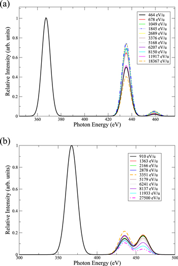
Figure 2. (a) Measured intensities of X-rays emitted by C5+ resulting from C6+ CX with He for various collision energies (Defay et al. 2013). (b) Same as (a), but for C6+ CX with H2 (Fogle et al. 2014). Spectra are produced using a Gaussian FWHM of 5 eV for all collision energies.
Download figure:
Standard image High-resolution image
Figure 3. (a) Experimental X-ray spectrum emitted by C5+ following a CX collision of C6+ with He at a collision energy of 1049 eV u−1 (451 km s−1; Defay et al. 2013) compared to theoretical spectra produced using MCLZ low-energy and statistical ℓ-distribution cross sections as well as AOCC cross sections (Fritsch & Lin 1991) at the same energy. (b) Experimental X-ray spectrum for C6+ CX with H2 at 910 eV u−1 (420 km s−1; Fogle et al. 2014) compared to theoretical spectra produced using MCLZ low-energy and statistical ℓ-distribution cross sections. A Gaussian FWHM of 5 eV was used.
Download figure:
Standard image High-resolution imageFor the experimental spectra observed for C6+ collisions with H2 shown in Figure 2(b), while the Lyβ line is significantly smaller than that for the collision with He, the Lyγ line also contributes significantly to the spectrum for all collision energies. For this collision, the Lyβ and Lyγ peaks are largest for the collision energy of 3351 eV u−1. The theoretical spectrum calculated with the MCLZ statistical ℓ-distribution for the collision energy of 910 eV u−1, shown in Figure 3(b), is in excellent agreement with the experimental result.
Experiments for O7+ and O8+ were also performed with He and H2, but only at 3.11 keV u−1. Figures 4(a) and (b) compare these measurements with the MCLZ low-energy and statistical ℓ-distributions, respectively. For both systems, the statistical ℓ-distribution provided the best agreement with the low-energy ℓ-distribution being significantly larger for the Lyβ and higher lines. The statistical ℓ-distribution intensities are very close to lying within the error bars of the experiments for all lines. For collisions of O7+ with He and H2 shown in Figure 5, however, the agreement is less satisfactory. Unfortunately, due to the long lifetime of the  state, the experiment is unable to measure the forbidden line that results in a shift in the centroid of the experimental Kα line. While there is some discrepancy in the Kβ line intensity for He and Kγ line for H2, this may partly be due to the fact that these lines are not resolved in the measurements of Greenwood et al. (2001).
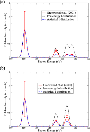
Figure 4. (a) X-ray spectral measurements for O7+ following O8+ CX with H2 at 3.11 keV u−1 (774 km s−1, Greenwood et al. 2001) compared to MCLZ calculation at the same energy. (b) Same as above, but for O8+ CX with He. While a Gaussian FWHM of 10 eV was adopted here, line ratios were extracted from emission measurements in Greenwood et al. (2001) with a Gaussian FWHM of ∼100 eV.
Download figure:
Standard image High-resolution image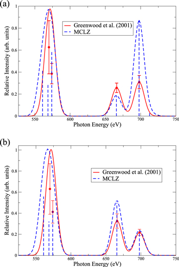
Figure 5. (a) X-ray spectral measurements performed by Greenwood et al. (2001) for O6+ following O7+ CX with H2 at 2.72 keV u−1 (724 km s−1) compared to MCLZ calculation at the same energy. (b) Same as above, but for O7+ CX with He. While a Gaussian FWHM of 10 eV was adopted here, line ratios were extracted from emission measurements in Greenwood et al. (2001) with a Gaussian FWHM of ∼100 eV.
Download figure:
Standard image High-resolution imageWhile the aim of these comparisons between theoretical methods and various measurements was to deduce trends to give some insight into the physics, to guide selection of the most reliable methods or data, and to provide some measure of confidence when predictions are made with simpler approaches, it turns out that nature is far more complicated. Using available experiments as benchmarks, it often is the case that simpler approaches give results in better agreement than perceived more robust methods. For H-like emission, results with ℓ-distribution functions are sometimes at odds with expectations and trends appear to be highly target-dependent. Experiments themselves often have limitations that hinder direct determination of desired parameters. Nevertheless, using what insights can be gleaned, a pragmatic approach is adopted to construct and test a comprehensive database as presented below. Improvements in computational and experimental methods are needed to advance the state of the database in the near future.
4. Velocity-dependent X-Ray Emission Modeling
Following previous work (Cumbee et al. 2014), updated XSPEC CX models of the Cygnus Loop were performed including more ions, targets, and collision energies. H- and He-like C, N, O, Ne, Mg, Al, and Si collisions with H and a 10% fraction of He were considered for collision energies from 200 eV u−1 (∼200 km s−1) to 5 keV u−1 (∼1000 km s−1). The best available cross sections were chosen for each collision energy and system based on agreement with previous theoretical results and benchmarking with experimental results. When other data are not available, the highest level of theory is chosen (i.e., the QMOCC method). The line ratios for each ion-H collision are presented in Table 2, while those for ion-He collisions are presented in Table 3, and those for ion-H2 collisions are given in Table 4.
Table 3. Charge Exchange X-Ray Emission with He Targets for SEC
| Line | Photon Energy | 200 eV u−1 | 300 eV u−1 | 500 eV u−1 | 700 eV u−1 | c1000 eV u−1 | 2000 eV u−1 | 3000 eV u−1 | 5000 eV u−1 |
|---|---|---|---|---|---|---|---|---|---|
| (eV) | (195.7 km s−1) | (239.7 km s−1) | (309.4 km s−1) | (366.1 km s−1) | (437.5 km s−1) | (618.8 km s−1) | (757.8 km s−1) | (978.4 km s−1) | |
| C v K α f | 298.96 | 2.5890 | 2.6085 | 2.6306 | 2.6434 | 2.6494 | 2.6739 | 2.6723 | 2.6394 |
| C v K α i | 304.41 | 0.2100 | 0.2121 | 0.2145 | 0.2157 | 0.2164 | 0.2187 | 0.2188 | 0.2162 |
| C v K α r | 307.90 | 1.0000 | 1.0000 | 1.0000 | 1.0000 | 1.0000 | 1.0000 | 1.0000 | 1.0000 |
| C v K β | 354.52 | 0.6122 | 0.6045 | 0.5967 | 0.5941 | 0.5890 | 0.5841 | 0.5784 | 0.5687 |
| O vii K α f | 560.99 | 2.0313 | 2.0317 | 1.9960 | 1.9591 | 1.8585 | 1.5048 | 1.2546 | 0.9920 |
| O vii K α i | 568.59 | 1.0309 | 1.0299 | 1.0137 | 1.0001 | 0.9619 | 0.8297 | 0.7344 | 0.6300 |
| O vii K α r | 573.95 | 1.0000 | 1.0000 | 1.0000 | 1.0000 | 1.0000 | 1.0000 | 1.0000 | 1.0000 |
| O vii K β | 665.62 | 0.4328 | 0.4530 | 0.5176 | 0.5938 | 0.7205 | 1.0512 | 1.2110 | 1.3184 |
| O vii K γ | 697.80 | 0.8981 | 0.8927 | 0.8703 | 0.8513 | 0.8028 | 0.6277 | 0.5037 | 0.3596 |
Note. Same as Table 2, but for collisions with He. AOCC cross sections are used for C6+ + He (Fritsch & Lin 1991) for most energies, but this table is primarily composed of MCLZ calculations.
Only a portion of this table is shown here to demonstrate its form and content. A machine-readable version of the full table is available.
Download table as: DataTypeset image
Table 4. Charge Exchange X-Ray Emission with H2 Targets for SEC
| Line | Photon Energy | 200 eV u−1 | 300 eV u−1 | 500 eV u−1 | 700 eV u−1 | 1000 eV u−1 | 2000 eV u−1 | 3000 eV u−1 | 5000 eV u−1 |
|---|---|---|---|---|---|---|---|---|---|
| (eV) | (195.7 km s−1) | (239.7 km s−1) | (309.4 km s−1) | (366.1 km s−1) | (437.5 km s−1) | (618.8 km s−1) | (757.8 km s−1) | (978.4 km s−1) | |
| C V K α f | 298.96 | 0.5756 | 0.4938 | 0.5521 | 0.6160 | 0.7039 | 0.9048 | 1.0284 | 1.1814 |
| C V K α i | 304.41 | 0.0649 | 0.0609 | 0.0679 | 0.0730 | 0.0784 | 0.0866 | 0.0904 | 0.0951 |
| C V K α r | 307.90 | 1.0000 | 1.0000 | 1.0000 | 1.0000 | 1.0000 | 1.0000 | 1.0000 | 1.0000 |
| C V K β | 354.52 | 4.5261 | 3.9612 | 3.4357 | 3.1980 | 2.9687 | 2.5877 | 2.3827 | 2.1224 |
| C V K γ | 370.92 | 0.0198 | 0.0075 | 0.0026 | 0.0015 | 0.0009 | 0.0004 | 0.0002 | 0.0001 |
Note. Same as Table 2, but for collisions with H2. This table is composed entirely of MCLZ calculations.
Only a portion of this table is shown here to demonstrate its form and content. A machine-readable version of the full table is available.
Download table as: DataTypeset image
In each of these tables, QMOCC cross sections are adopted, when available, for C5+ + H (Nolte et al. 2012), N6+ + H (Wu et al. 2011), and O7+ + H (J. L. Nolte et al. 2017, in preparation). AOCC cross sections were then adopted for Ne10+ + H for energies above 1 keV u−1, and for C6+ + He (Fritsch & Lin 1991) for most energies. For C6+ + H and O8+ + H, recommended cross sections from Janev et al. (1993) were adopted, and for N7+ + H (Harel et al. 1998), MOCC cross sections were used. In all other cases, and when energies are missing for other methods, MCLZ cross sections are adopted. For bare ion collisions, below 1 keV u−1, MCLZ low-energy ℓ-distribution cross sections were used, and for energies at and above 1 keV u−1, MCLZ statistical ℓ-distribution cross sections are adopted. All of these cross sections can be found in the Kronos Database (Mullen et al. 2016, 2017).
Pure CX spectra are shown for each collision energy in Figure 6, with the assumption that all ions considered here have the same abundance. In this case, all ion-neutral spectra are normalized by the sum of the total X-ray spectrum so that the sums of all Lyα+ lines and all Kα+ lines are equal to 1. The 1 keV u−1 spectrum is highlighted in black for comparison to the model discussed in Cumbee et al. (2014). A line-ratio plot for the lowest collision energy of 200 eV u−1 is also shown. A Gaussian FWHM resolution of 50 eV was chosen in order to more clearly highlight the variation in velocity. At the lowest photon energies (below ∼600 eV), the velocity plays a very important role in the intensity of the spectra. In this region, only C, N, and O ions contribute to the spectra, and a dramatic increase in the intensity from the lowest collision energy (200 eV u−1) to the highest collision energy (5000 eV u−1) is clear, especially near 600 eV photon energies. It is important to note that for these ions, QMOCC and recommended cross sections are used, indicating that this velocity variation is not dominated by uncertainties in the atomic data or having to choose an ℓ-distribution for the MCLZ cross sections.
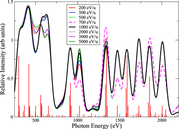
Figure 6. CX X-ray emission line ratios from H-like and He-like C-Si ions following CX collisions with H and a 10% fraction of He, with the sum of all lines in each spectrum having a normalization of 1, indicating a similar abundance for each initial ion. These spectra are shown to emphasize the variation in intensity caused by the collision velocity and are for illustrative purposes only. Detailed spectral data including line ratios (impulses) are presented in Tables 2 and 3, and can be found in the Kronos database. A line-ratio plot is shown in red for 200 eV u−1. The line ratios are convolved with a 50 eV FWHM Gaussian to produce the spectra shown.
Download figure:
Standard image High-resolution imageThe Ne10+ Lyα line displays a very strong fluctuation in intensity for velocities corresponding to ∼1000 eV (based on data primarily from AOCC, CTMC, and MCLZ cross sections), while the strong velocity variation at ∼1300 eV is primarily due to Mg11+ collisions, calculated with MCLZ cross sections. At ∼1500 eV, however, the spectra of the eight collision energies converge to one of two forms: the low-energy ℓ-distribution or the statistical ℓ-distribution in the MCLZ method. In Figure 6, because of this convergence, the four lower-collision-energy spectra are overlaid so that only the 700 eV u−1 spectrum is visible, and the four higher-collision-energy spectra are overlaid so that only the 1000 eV u−1 spectrum is visible. For the ions that contribute to the spectra at these energies (Mg, Al, and Si), only MCLZ CX calculations are available. Tables 2 and 3 show that for the H-like ions, the relative intensity of each line only varies by a small amount both below 700 eV u−1, for which the low-energy ℓ-distribution cross sections are used, and above 1000 eV u−1, for which only the statistical ℓ-distribution cross sections are used. There is, however, a significant variation between the line ratios produced with these two ℓ-distributions. For the He-like emission, such as Al12+, for which no ℓ-distribution is necessary, each line only varies slightly for the entire collision energy range, which is highlighted in Figure 6 at ∼1550 eV, for which all spectra have the same intensity. Finally, there are prominent emission deficient windows near 750 and 1250 eV. These windows might be partially filled in by multi-electron, high-charge ion emission not considered here (see below). However, these ions mostly contribute to the soft X-ray region below 500 eV. Clearly, the velocity dependence shown here can make a significant difference in modeling of X-ray observations.
In order to explore the contribution to the X-ray emission spectrum of the Cygnus Loop from CX due to these ions colliding with H and He, the model results described above were incorporated into an XSPEC model, enhancing the model described by Cumbee et al. (2014), which only included C, N, and O ions colliding with H. Figure 7 shows the best fit of this model from XSPEC for the collision energy of 2 keV u−1. The best fit for this model, similar to Figure 3 in Cumbee et al. (2014), was still unable to account for the X-ray-enhanced region near 0.72 keV, as hinted at by the gap at that photon energy in Figure 7. This fit has a reduced  of 3.7, which is a slight improvement over the reduced
  of 3.95 obtained in Figure 3 in Cumbee et al. (2014). Two unconstrained lines, mimicking CX due to Fe16+ collisions, were then added as done in Figure 4 in Cumbee et al. (2014), since CX data are not currently available for this ion. This resulted in a much better fit with a reduced
  of 1.91 as shown in Figure 8. The quality of the fit is similar to that displayed in Figure 4 in Cumbee et al. (2014), suggesting that the addition of Ne, Mg, Al, and Si lines due to CX does not significantly improve the Cygnus Loop model.
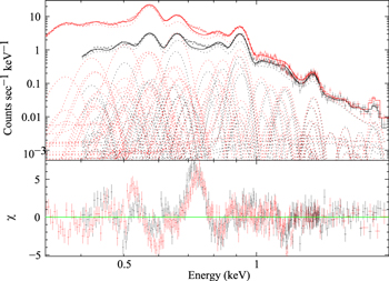
Figure 7. Spectrum (crosses) from the NE4 outermost rim of the Cygnus Loop as described in Figure 3(a) of Cumbee et al. (2014) but with additional lines including Ne-Si ions and collisions with both H and a 10% fraction of He for a collision energy of 2 keV u−1. The BI spectrum is red and the FI spectrum is black. Residuals are shown in the lower panel with a reduced  of 3.7 with 579 dof.
Download figure:
Standard image High-resolution image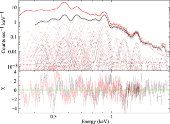
Figure 8. Same as Figure 7, but with the addition of Fe L-shell lines at 0.726 and 0.822 keV. Also shown is a reduced  of 1.91 with 577 dof.
Download figure:
Standard image High-resolution imageA similar model was then performed for 200 eV u−1, 300 eV u−1, 500 eV u−1, 700 eV u−1, 1 keV u−1, 3 keV u−1, and 5 keV u−1. The XSPEC line normalizations for the Lyα and Kα resonant lines were then extracted for all models, and are shown in Table 5. These Lyα and Kα resonant line normalizations, along with the line ratios that form the rest of the spectra in Tables 2 and 3, are then used to produce synthetic spectra that include only the contribution of CX in the Cygnus Loop. Figure 9 shows these synthetic spectra using a Gaussian FWHM of 10 eV, and Figure 10 shows these synthetic spectra using a Gaussian FWHM of 50 eV in order to more clearly highlight the intensity variation of the spectra for the different velocities. Table 5 also indicates the reduced  for each collision energy, and for these models, the best fits occurred with a reduced
  of 3.75 at 1 keV u−1 and 2 keV u−1, with 3 keV u−1 and 5 keV u−1 being close with a reduced
  of 3.8. The fits below 1 keV u−1 were relatively poor, with the best fit having a reduced
  of 4.37 at 500 eV u−1. Figure 10 shows that the CX spectra greatly vary around 500 and 650 eV, indicating the X-ray bands most sensitive to velocity variations.

Figure 9. CX X-ray emission spectra and line intensity ratios (vertical red lines, at 200 eV u−1) for H-like and He-like C-Si ions colliding with H and a 10% fraction of He extracted from XSPEC fits of the Cygnus Loop, as shown in Figure 7 using 10 eV Gaussian FWHM.
Download figure:
Standard image High-resolution image
Figure 10. Same as Figure 9, but using a 50 eV Gaussian FWHM resolution.
Download figure:
Standard image High-resolution imageTable 5. XSPEC Model Line Normalizations for Charge Exchange with H and 10% He
| Line | Energy | 200 eV u−1 | 300 eV u−1 | 500 eV u−1 | 700 eV u−1 | 1000 eV u−1 | 2000 eV u−1 | 3000 eV u−1 | 5000 eV u−1 |
|---|---|---|---|---|---|---|---|---|---|
| (eV) | (195.7 km s−1) | (239.7 km s−1) | (309.4 km s−1) | (366.1 km s−1) | (437.5 km s−1) | (618.8 km s−1) | (757.8 km s−1) | (978.4 km s−1) | |
| C VI Ly α | 367.49 |

|

|

|

|

|

|

|

|
| N VI K α r | 430.70 |

|

|

|

|

|

|

|

|
| NV II Ly α | 500.28 |

|

|

|

|

|

|

|

|
| O VII K α r | 573.95 |

|

|

|

|

|

|

|

|
| O VIII Ly α | 653.56 |

|

|

|

|

|

|

|

|
| Ne IX K α r | 922.02 |

|

|

|

|

|

|

|

|
| Ne X Ly α | 1021.65 |

|

|

|

|

|

|

|

|
| Mg XI K α r | 1352.25 |

|

|

|

|

|

|

|

|
| Mg XII Ly α | 1472.00 |

|

|

|

|

|

|

|

|
| Al XII K α r | 1598.30 |

|

|

|

|

|

|

|

|
| Al XIII Ly α | 1728.10 | 0.314
|

|

|

|

|

|

|

|
| Si XIII K αr | 1864.99 |

|

|

|

|

|

|

|

|
reduced 
|
4.42216 | 4.48461 | 4.37430 | 4.47987 | 3.75379 | 3.75379 | 3.84641 | 3.81405 | |
Note. All Kα resonant and Lyα normalizations are shown for the process of CX in the Cygnus loop. Any normalizations for collisions with He are multiplied by 0.10 to simulate a ∼10% abundance of He relative to H. Lyα and Kβ and higher lines are provided in Tables 2–4.
Download table as: ASCIITypeset image
Two lines mimicking Fe L-shell emission at 0.726 and 0.822 keV were then added to the CX models for each energy. The Lyα and Kα resonant line intensities as determined by XSPEC are shown in Table 6, and the synthetic spectra with the addition of the Fe L-shell lines are shown in Figure 11. While the line at 0.726 keV makes a significant contribution to the spectrum (highlighted in black in the figure), the line at 0.822 keV makes no contribution. Katsuda et al. (2011) note, however, that these two lines usually have similar intensities. Thus, realistic CX line ratios must be included in the CX model in the future in order to determine how Fe16+ CX will affect the spectra.
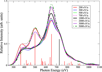
Figure 11. Same as Figure 10 (using a 50 eV Gaussian FWHM resolution), but including two lines at 0.726 keV and 0.822 keV to mimic Fe L-shell CX emission. The 2 keV u−1 XSPEC fit is shown in Figure 8. The Fe line at 0.726 is shown in black in the impulse spectrum for the collision energy of 200 eV u−1.
Download figure:
Standard image High-resolution imageTable 6. XSPEC Model Line Normalizations for Charge Exchange with H and 10% He with Fe L-shell Lines
| Line | Energy | 200 eV u−1 | 300 eV u−1 | 500 eV u−1 | 700 eV u−1 | 1000 eV u−1 | 2000 eV u−1 | 3000 eV u−1 | 5000 eV u−1 |
|---|---|---|---|---|---|---|---|---|---|
| (eV) | (195.7 km s−1) | (239.7 km s−1) | (309.4 km s−1) | (366.1 km s−1) | (437.5 km s−1) | (618.8 km s−1) | (757.8 km s−1) | (978.4 km s−1) | |
| C VI Ly α | 367.49 |

|

|

|

|

|

|

|

|
| N VI K α r | 430.70 |

|

|

|

|

|

|

|

|
| N VII Ly α | 500.28 |

|

|

|

|

|

|

|

|
| O VII K α r | 573.95 |

|

|

|

|

|

|

|

|
| O VIII Ly α | 653.56 |

|

|

|

|

|

|

|

|
| Ne IX Kα r | 922.02 |

|

|

|

|

|

|

|

|
| Ne X Ly α | 1021.65 |

|

|

|

|

|

|

|

|
| Mg XI K α r | 1352.25 |

|

|

|

|

|

|

|

|
| Mg XII Ly α | 1472.00 |

|

|

|

|

|

|

|

|
| Al XII K α r | 1598.30 |

|

|

|

|

|

|

|

|
| Al XIII Ly α | 1728.10 |

|

|

|

|

|

|

|

|
| Si XIII K α r | 1864.99 |

|

|

|

|

|

|

|

|
Fe L( ) ) |
0.726 |

|

|

|

|

|

|

|

|
Fe L( ) ) |
0.822 |

|

|

|

|

|

|

|

|
reduced 
|
2.47466 | 2.38022 | 2.34961 | 2.45434 | 2.27481 | 1.92810 | 1.92810 | 1.93168 | |
Note. Same as Table 5, but with new XSPEC fits including two additional lines to mimic CX for Fe16+ collisions at 0.726 and 0.822 keV.
Download table as: ASCIITypeset image
5. Heliospheric Line-ratio Comparisons
This CX model can also be applied to solar wind charge exchange (SWCX) with heliospheric neutrals in order to improve our understanding of the soft X-ray background. In order to have a realistic solar wind CX model, the ion composition and velocity of the solar wind and the neutral composition of the heliosphere must be considered. The solar wind can roughly be described as having two modes, the fast solar wind at ∼750 km s−1 is emitted from coronal holes in the Sun near solar minimum, and the slow solar wind at ∼400 km s−1 is emitted from low solar latitudes. While these solar wind modes have different velocities, they also have very different compositions, as described by Schwadron & Cravens (2000). The slow solar wind has a higher abundance of various ionization stages including H- and He-like C, N, and O described in this paper, while the fast solar wind contains He-like C, N, and O, but only H-like C. The solar wind ion composition includes C through Fe ions, but for ions other than C, N, and O, the H-like and He-like ionization stages make little to no contribution to the solar wind ion flux.
Differences in X-ray emission spectra due to variations in the solar wind velocities and elemental ionization fractions, as well as heliospheric neutral abundance variations, can be directly probed through detailed SWCX modeling. A model spectrum, arising from consideration of a limited range of ions in the solar wind (H-like and He-like C, N, and O) colliding with H and a 10% fraction of He, is shown in Figure 12. In this case, the relative abundances of the ions (relative to O), from Schwadron & Cravens (2000), are adopted and shown in Table 7. In this scenario, the fast solar wind has the most X-ray flux at the lowest energies, while the slow solar wind contributes significantly throughout the entire spectrum. In order for this to be a realistic SWCX model, lower ionization stages, including those of heavier elements (e.g., Si, Mg, Ne, etc.) present in the solar wind, must be considered and will influence the spectrum below 500 eV.
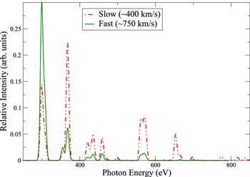
Figure 12. Theoretical X-ray emission lines for H-like and He-like C, N, and O ions colliding with H and a fraction of 10% He for the fast solar wind (∼750 km s−1) and slow solar wind (∼400 km s−1). A Gaussian FWHM of 10 eV is used.
Download figure:
Standard image High-resolution imageTable 7. Abundance Ratios (Relative to O) for Ions in the Solar Wind
| Fast | Slow | |
|---|---|---|
| Ion | Solar Wind | Solar Wind |
| C5+ | 0.440 | 0.210 |
| C6+ | 0.085 | 0.318 |
| N6+ | 0.011 | 0.058 |
| N7+ | 0 | 0.006 |
| O6+ | 0.970 | 0.730 |
| O7+ | 0.030 | 0.200 |
| O8+ | 0 | 0.070 |
Note. Abundance ratios from Schwadron & Cravens (2000). While O6+ abundances are provided in this table to indicate the total abundance of O, they are not included in CX models here.
Download table as: ASCIITypeset image
Bodewits et al. (2007) produced a velocity-dependent theoretical X-ray emission model relevant to the solar wind CX mechanism for H-like and He-like C, N, and O CX collisions, but only with H, as shown in their Table 2. This model used realistic CX cross sections before applying a cascade model similar to that described here. Their Table 2 provides a set of emission cross sections, which can be compared to our relative line ratios by normalizing each emission cross section to the respective Lyα or Kα resonant line, as shown in Table 8 for the collision energies of 200 and 1000 eV u−1. The line-ratio models are somewhat similar for most lines, with the largest percent difference occurring for the N vi and O vii Kδ lines at 200 eV u−1 and the N vii Lyδ line and the O vii K line for 1000 eV u−1. The H-like line ratios are more similar than the He-like line ratios for both energies. The more recent QMOCC cross sections for the He-like ions, which are considered in this paper, are likely more accurate for C5+ (Nolte et al. 2012), N6+ (Wu et al. 2011), and O7+ (J. L. Nolte et al. 2017, in preparation).
Table 8. Comparison of Normalized Line Ratios to Bodewits et al. (2007) for H Targets
| Photon Energy | 200 eV u−1 | 1000 eV u−1 | |||||
|---|---|---|---|---|---|---|---|
| Line | (eV) | Bodewits | This work | % Difference | Bodewits | This work | % Difference |
| C v K α f | 298.9600 | 4.8333 | 5.7749 | 17.7516 | 3.8462 | 3.5342 | 8.4536 |
| C v K α i | 304.4100 | 0.3611 | 0.5253 | 37.0458 | 0.3462 | 0.2980 | 14.9510 |
| C v K α r | 307.9000 | 1.0000 | 1.0000 | 0.0000 | 1.0000 | 1.0000 | 0.0000 |
| C v K β | 354.5200 | 0.3056 | 0.4950 | 47.3282 | 0.2500 | 0.3282 | 27.0495 |
| C v K γ | 370.9200 | 0.3889 | 0.0704 | 138.6878 | 0.1385 | 0.0574 | 82.7743 |
| C v K δ | 378.5300 | 0.0000 | 0.0000 | ⋯ | 0.0077 | 0.0000 | ⋯ |
| C vi Ly α | 367.4900 | 1.0000 | 1.0000 | 0.0000 | 1.0000 | 1.0000 | 0.0000 |
| C vi Ly β | 435.5500 | 0.1067 | 0.1229 | 14.1426 | 0.1412 | 0.1478 | 4.5841 |
| C vi Ly γ | 459.3700 | 0.1933 | 0.1525 | 23.6145 | 0.1765 | 0.2286 | 25.7384 |
| C vi Ly δ | 470.3900 | 0.0367 | 0.0283 | 25.7568 | 0.0159 | 0.0140 | 12.5984 |
| C vi Ly |
476.3800 | 0.0000 | 0.0006 | ⋯ | 0.0000 | 0.0012 | ⋯ |
| N vi K α f | 419.8000 | 3.4211 | 5.2080 | 41.4170 | 3.4118 | 3.1960 | 6.5306 |
| N vi K α i | 426.3200 | 0.7105 | 0.9454 | 28.3676 | 0.7059 | 0.9958 | 34.0742 |
| N vi K α r | 430.7000 | 1.0000 | 1.0000 | 0.0000 | 1.0000 | 1.0000 | 0.0000 |
| N vi K β | 497.9700 | 0.1132 | 0.1765 | 43.7358 | 0.1529 | 0.1719 | 11.6727 |
| N vi K γ | 521.5800 | 0.2132 | 0.1384 | 42.5295 | 0.2000 | 0.0931 | 72.9444 |
| N vi K δ | 532.6500 | 0.0368 | 0.0012 | 187.3824 | 0.0165 | 0.0101 | 47.9522 |
| N vii Ly α | 500.2800 | 1.0000 | 1.0000 | 0.0000 | 1.0000 | 1.0000 | 0.0000 |
| N vii Ly β | 592.9300 | 0.1575 | 0.1214 | 25.8874 | 0.1024 | 0.3453 | 108.5233 |
| N vii Ly γ | 625.3500 | 0.0725 | 0.0463 | 44.1077 | 0.1095 | 0.6163 | 139.6417 |
| N vii Ly δ | 640.3600 | 0.2750 | 0.2538 | 8.0182 | 0.0524 | 0.3265 | 144.6993 |
| N vii Ly |
648.5200 | 0.0000 | 0.0115 | ⋯ | 0.0019 | 0.0000 | ⋯ |
| O vii K α f | 560.9900 | 3.7374 | 1.9706 | 61.9055 | 3.1000 | 1.0928 | 95.7451 |
| O vii K α i | 568.5900 | 1.0101 | 1.2546 | 21.5922 | 0.9700 | 0.9547 | 1.5899 |
| O vii K α r | 573.9500 | 1.0000 | 1.0000 | 0.0000 | 1.0000 | 1.0000 | 0.0000 |
| O vii K β | 665.6200 | 0.1717 | 0.1784 | 3.8175 | 0.1200 | 0.1278 | 6.2954 |
| O vii K γ | 697.8000 | 0.0818 | 0.0794 | 2.9999 | 0.1300 | 0.0461 | 95.2868 |
| O vii K δ | 712.7200 | 0.2828 | 0.0209 | 172.4754 | 0.0540 | 0.0161 | 108.1312 |
| O vii K |
720.8400 | 0.0000 | 0.0116 | ⋯ | 0.0020 | 0.0077 | 117.5258 |
| O viii Ly α | 653.5600 | 1.0000 | 1.0000 | 0.0000 | 1.0000 | 1.0000 | 0.0000 |
| O viii Ly β | 774.5900 | 0.0963 | 0.1281 | 28.3460 | 0.0943 | 0.1212 | 24.9238 |
| O viii Ly γ | 816.9500 | 0.0370 | 0.0742 | 66.8176 | 0.0434 | 0.0553 | 24.1220 |
| O viii Ly δ | 836.5500 | 0.0889 | 0.1160 | 26.4642 | 0.0698 | 0.1113 | 45.8157 |
| O viii Ly |
847.2000 | 0.0593 | 0.0478 | 21.4073 | 0.0126 | 0.0184 | 37.1019 |
Download table as: ASCIITypeset image
In order to determine the effect that the neutral He to H fraction has on the total spectrum, that fraction was varied for each collision energy by multiplying each normalized spectrum (for each ion-neutral combination) by the fractional percentage (0% He to 75% He), and then summing the ion-H and ion-He line-ratio spectra, as shown in Figure 13. In this case, as the fraction of He varied from 0% He (100% H) to 75% He (25% H), the total intensities of the lines changed, through all energies shown, but particularly near 500 eV. This indicates that it can be important to consider the contribution from various neutral targets when considering CX collisions.

Figure 13. Theoretical X-ray emission lines for H-like and He-like C-Si ions colliding at 1 keV u−1 with H and varying the fraction of He from 0% He (100% H) to 75% He (25% H). Each individual model spectrum is normalized so that the sum of all lines is 1, and the black line shown with a fraction of 10% He can be compared to the black line shown in Figure 6 with the same collision energy. A Gaussian FWHM of 10 eV is used.
Download figure:
Standard image High-resolution image
6. Conclusions
A set of theoretical cross sections was prepared and line ratios were produced for the collisions of bare and H-like C-Si ions with H, He, and H2, drawing primarily from the results of the MCLZ method, supplemented by the results of the QMCOCC, AOCC, and CTMC methods when available. These data were compared to available experiments and other calculations. An X-ray emission model for use in XSPEC was prepared for eight collision energies; 200 eV u−1, 300 eV u−1, 500 eV u−1, 700 eV u−1, 1000 eV u−1, 2000 eV u−1, 3000 eV u−1, and 5000 eV u−1 using the best available methods as judged by this comparison of available data.
The velocity dependence of CX is shown to have a major impact on the fitted spectrum. All data are available in the Kronos database (Mullen et al. 2016, 2017) and on the UGA Charge Transfer Database (https://www.physast.uga.edu/ugacxdb/), including scripts to generate CX input for XSPEC. The databases are being continually updated as new CX data become available.