


Abstract
We present an analysis of the internal bulk rotation in the metal-poor globular cluster (GC) NGC 5024 (M53) using radial velocities (RVs) of individual cluster members. We use RV measurements from a previous abundance study of M53 done using the Hydra multi-object spectrograph on the WIYN 3.5 m telescope. The Hydra sample greatly increases the number of RVs available in the central regions of the cluster where the internal rotation is the strongest. The sample of cluster members is further increased through two previous kinematic studies of M53. The combined total sample contains 245 cluster members. With our sample, we are able to create a velocity dispersion profile of the cluster and derive a central velocity dispersion  we find that M53 inner regions are characterized by a peak amplitude of rotation equal to
  corresponding to a relatively high value of the ratio of the rotation speed to central velocity dispersion (
 ). Our data also reveal a radial variation in the orientation of the projected rotation axis suggesting complex internal kinematics.
Export citation and abstract BibTeX RIS
1. Introduction
Many recent observational studies are revealing an increasingly complex picture of globular clusters' (GCs) stellar content and dynamical properties. Large-scale photometric programs, such as the Hubble UV Legacy Survey (Piotto et al. 2015; Milone et al. 2017), and detailed spectroscopic studies (see Gratton et al. 2012 and references therein) have shown that they exhibit abundance patterns and color–magnitude diagram morphologies indicative of chemically distinct populations. The physical morphologies and dynamical properties of GCs have also shown that they deviate from the spherically symmetric and non-rotating systems they were once considered to be (King 1966). Most GCs have been shown to have some degree of elongation (White & Shawl 1987; Chen & Chen 2010) and an increasing number of7 them exhibit substantial internal rotation (see, e.g., Lane et al. 2011; Bellazzini et al. 2012; Fabricius et al. 2014; Kacharov et al. 2014; Kimmig et al. 2015; Cordero et al. 2017; Johnson et al. 2017). The discovery of an increasing number of stellar streams associated with GCs (see, e.g., Leon et al. 2000; Odenkirchen et al. 2001; Grillmair & Dionatos 2006; Grillmair & Johnson 2006; Küpper et al. 2015; Bernard et al. 2016) has also highlighted their contribution to the assembly history of the Galactic halo (see, e.g., Martell & Grebel 2010; Vesperini et al. 2010; Schaerer & Charbonnel 2011) and the effects of their interactions with the Milky Way.
The interplay between these complex GC characteristics provides important constraints for our current theories of cluster formation and evolution. Here, we present an analysis of the internal rotation in NGC 5024 (M53). M53 is a metal-poor cluster near the northern Galactic cap with a galactocentric radius  . Only ∼500 pc away, based on its Galactic X, Y, Z coordinates (Harris 1996, 2010 Version), is the GC NCG 5053. Together, and individually, these clusters provide a unique laboratory to test our understanding of GC evolution, especially regarding the subtle nexus between internal and external physical ingredients. These two GCs have very different morphologies, structural properties, and masses, despite currently experiencing the same Galactic potential; NGC 5053 is a loose, low-mass cluster, and M53 is a highly concentrated, high-mass cluster. These two clusters provide an opportunity to explore the interplay between Galactic potential, cluster concentration, and mass and how they are related.
Previous wide-field photometric surveys of these clusters have discovered a 6◦ tidal tail associated with NGC 5053 (Lauchner et al. 2006) and a possible "halo" of stars around M53 (Chun et al. 2010). Chun et al. (2010) also claimed to have detected a tidal bridge-like structure between NGC 5053 and M53, but this finding was not confirmed by Jordi & Grebel (2010). Additionally, M53 is suggested to be composed mostly of first generation (FG) stars, based on the morphology of its horizontal branch (Caloi & D'Antona 2011). This suggestion was further supported by our M53 abundance study (Boberg et al. 2016), where we concluded the FG stars make up ∼70% of the cluster members based on Na and O abundances (but see Milone et al. (2017) for a different estimate of the FG fraction from HST UV observations).
This study is part of our ongoing effort to create a comprehensive understanding of the chemical and dynamical evolution of this GC system. In Section 2, we provide a brief summary of the radial velocities (RVs) we measured as part of our abundance study in M53. We also describe how these data are combined with literature samples and their characteristics. In Section 3, we describe the method used to measure the internal rotation in the cluster. In Section 4, we present the results of our rotation analysis and compare them to previous rotation studies in M53. In Section 5, we provide a discussion of the results and our conclusions from this study. We also present how these results will be combined with forthcoming wide-field photometry of M53.
2. Data
2.1. Hydra Data
In Boberg et al. (2016), we completed an abundance study of M53 using medium-resolution (R ≈ 18,000) spectra of red giant branch (RGB) stars in the cluster using the Hydra Multi-object spectrograph on the WIYN3
3.5 m telescope. The RVs of our science targets were also measured to determine cluster membership and remove photometric interlopers from the sample. Multiple RV standards were observed at the beginning of each night when the Hydra spectra were collected. By measuring the RVs of our science targets against multiple standards, we found that the mean standard deviation of the individual measurements is 0.1  , and they have a mean error of 1.1
  . The inter-night RV measurements of our sample were very stable with a mean standard deviation of 0.41
  . A full description of the methods used to measure the RVs is given in Boberg et al. (2016). In total, the Hydra sample contains 74 stars with a mean velocity of
  , with a standard error on the mean of
  . This value is consistent with the value found by Kimmig et al. (2015) (
 ). We will show that the Hydra sample is crucial to measuring the internal rotation of M53 because it covers the innermost regions of the cluster. This sample has 12 stars within two times the core radius (
 ) and 49 stars within two times the half-light radius (
 ). A summary of the characteristics of the Hydra sample is given in Table 1. The structural parameters are taken from Harris (1996; 2010 Version).
Table 1. RV Sample Comparisons
| Study | Sample Size | Mean RV | Mean RV Error | Median Radius (r) |
|---|---|---|---|---|
( ) ) |
( ) ) |
(arcminutes) | ||
| (1) | (2) | (3) | (4) | (5) |
| Boberg et al. (2016) | 73 | −63.35 | 1.16 | 1.73 |
| Kimmig et al. (2015) | 91 | −63.43 | 0.33 | 6.85 |
| Lane et al. (2011) | 81 | −63.64 | 3.40 | 4.49 |
Download table as: ASCIITypeset image
2.2. Literature Samples
The Hydra sample provides good coverage of the innermost regions of M53. In order to expand our sample to larger radii and increase the sample size, we combine our Hydra sample with the data from two previous studies (Lane et al. 2011; Kimmig et al. 2015). The RVs taken from Lane et al. (2011) were determined from low- (R = 3700) and medium-resolution (R = 10000) spectra taken with the AAOmega spectrograph on the Anglo-Australian Telescope. The Kimmig et al. (2015) RVs were determined from relatively high resolution (R ∼ 38,000) spectra taken with the Hectochelle spectrograph on the Multiple Mirror Telescope. There are 11 and 15 stars in common between the Hydra sample and those from Kimmig et al. (2015) and Lane et al. (2011), respectively. In Figure 1 we plot RVs of stars in common between Kimmig et al. (2015) and Lane et al. (2011) versus their measured RVs in the Hydra sample. There is generally good agreement between the three studies, but the Kimmig et al. (2015) and Lane et al. (2011) RVs are systematically higher than those measured in our Hydra study. We find the following mean differences between the Hydra RVs, and those measured by Lane et al. (2011) and Kimmig et al. (2015):  ,
, 
 ,
,  . These mean offsets are added to the RVs of their respective studies to put them on the same relative scale as the Hydra sample. Stars in common with either study are assigned the RV as found from the Hydra data rather than averaging the different RV measurements from each study. The 44 stars in common between Kimmig et al. (2015) and Lane et al. (2011) were assigned the value as found by Kimmig et al. (2015) due to their typically lower measurement errors. The Kimmig et al. (2015) catalog did not include a cluster membership label. Possible cluster nonmembers were removed by only including stars in the following RV range:
  . These limits represent the approximate 3σ level of the entire sample and brought the combined RV catalog to 250 stars. We also calculated the absolute value of the difference of each RV with the systemic velocity of the cluster as defined by these 250 stars. If this difference was greater than the 98th percentile of difference distribution, the star was removed from the sample. This was done to remove relatively extreme RVs that might skew the rotation analysis. After this cut, the RV catalog contained 245 stars. In Table 1, we summarize how each sample contributes to the final RV catalog used in this study. The previously mentioned offsets were applied before calculating the statistics shown in Table 1.

Figure 1. Comparison of the RVs for stars in the study in common with Kimmig et al. (2015) and Lane et al. (2011). The error bars on the points are the errors reported by each study. The solid black line is a one-to-one relationship that has not been fit to the data.
Download figure:
Standard image High-resolution imageIn Figure 2, we plot the cumulative radial distribution of each sample in the cluster. This figure clearly illustrates the benefit and importance of the Hydra sample. The Kimmig et al. (2015) and Lane et al. (2011) samples only have 10 and 17 stars within  , respectively, and neither sample has any stars within
  . An integral field unit (IFU) study of the central rotation in GCs by Fabricius et al. (2014) found that all 11 clusters in their sample, including M53, show significant signatures of internal rotation. The IFU used by Fabricius et al. (2014) covered each cluster out to a radius of
  , which, in the case of M53, corresponds to
  . The Hydra sample allows us to measure and constrain the internal rotation within M53 using individual RVs in a region that bridges the radial gap between the regions covered by Fabricius et al. (2014) and those probed by Kimmig et al. (2015) and Lane et al. (2011). The relatively large sample (N = 48) of Hydra stars within 2rh provides the essential data needed to measure the central dynamics of the cluster where the signatures of internal rotation may be more pronounced.

Figure 2. Cumulative radial distribution of the three samples used in this study. Here, we assume a half-light radius of 1.3 arcmin and a core radius of 0.35 arcmin (Harris 1996, 2010 Version).
Download figure:
Standard image High-resolution image3. Observational Analysis
3.1. Rotation
We implement a commonly used method to detect rotation in M53 based on individual line-of-sight RV measurements (Cote et al. 1995; Lane et al. 2009; Bellazzini et al. 2012; Bianchini et al. 2013). The sample of cluster members is divided by a line passing through the center of the cluster. The difference ( ) between the mean RV of the stars on either side of the line is calculated and becomes the amplitude of rotation at that position angle (PA). The dividing line is then rotated to a new PA and the difference is recalculated. This process is repeated until the PAs have swept out a full 360◦. We define
  to be to the right (east) and
  to be pointing up (north). The PA values are increased in steps of 15◦ moving counter clockwise. The resulting curve of
  as a function of PA is then fit by the sine law shown in Equation (1),

We determine the amplitude of rotation in the cluster Arot and the phase (ϕ) of the sine curve by fitting this model to the rotation curve. The axis of rotation of the cluster, PA0, is related to the phase of the sine model by  and is the PA that corresponds to the maximum in the rotation curve. This procedure was also repeated with the PA increasing in steps of
  , and 20◦. We found that changing the step size in PA did not have a large effect on the fit axis of rotation, which varied by only
  among the step sizes we tested. As noted in Lane et al. (2010a), this method and fit results in an amplitude (Arot) that is twice the actual velocity of rotation in the cluster. We note that in a number of studies, Arot is adopted as a measure of the rotation amplitude instead of
  to account for the effects of the radial variation of the rotational velocity (see, e.g., Bellazzini et al. 2012). The amplitude of rotation is also affected by the inclination (i) of the cluster by a factor of sin(i), which is not measurable in GCs. Therefore, the amplitude of rotation we measure with this method is a lower limit of the actual intrinsic rotation in the cluster.
Following the example of Kacharov et al. (2014), we use the maximum likelihood method outlined in Walker et al. (2006) to calculate mean velocity and velocity dispersions of different stellar samples in our analysis (e.g., the mean velocity on either side of the cluster dividing line). We numerically determine these values by maximizing the log-likelihood formula shown in Equation (2) (Equation (8) in Walker et al. 2006) using the Metropolis–Hastings algorithm (Hastings 1970). In this equation, vi and  are the individual measured RVs and their errors, respectively. By maximizing this log-likelihood, we can determine the mean RV of a given population
  , as well as its intrinsic velocity dispersion
  . This method allows us to take the measurement error, and RV dispersion, into account when determining these characteristics of a given sample.
3.2. Bootstrap Analysis
We implemented a bootstrap/Monte Carlo method in order to characterize the variation in the fit model parameters Arot and PA0. For each RV measurement in the sample, we added a noise value randomly drawn from a normal distribution centered on zero with a standard deviation equal to the error on that RV measurement. We then ran the noise-added RVs through the rotation-curve procedure outlined in Section 3.1 and redetermined the fit parameters. This process was then repeated 200 times. The procedure also provided us with a measure of the variation of  at a given PA. From this analysis we found that the average standard deviation of
  is
is  .
.
4. Results
4.1. Rotation Curves
We performed the rotation analysis on subsets of stars that fell within a maximum distance (rmax) from the cluster center. This is done to characterize how the axis and amplitude of rotation vary as a function of radius similar to the analysis in Bianchini et al. (2013). The max radii used ranged from  in steps of 0.25. This analysis was done on the total combined data set, as well as just the RV sample from Hydra.
In Table 2, we list a subset of the Arot and PA0 values resulting from performing the rotation-curve analysis on different samples of stars. Column 1 gives the rmax values used to define each sample. Columns 2–4 give the number of stars, fit amplitude of rotation, and fit axis of rotation, respectively, while columns 5–7 give these same values for the Hydra-only sample. In Figure 3, we plot the rotation curves resulting from  . The column of panels on the left are the rotation curves for the total combined sample, and the column of panels on the right are the rotation curves for the Hydra-only sample. The last panel in each column shows the rotation curve for each sample when no radius cut is applied and all stars are used. The rotation curves have a peak amplitude of
  and
and  for the total combined and Hydra-only samples, respectively, for stars within 2rh. As mentioned earlier, the rotational velocity, Vrot, is equal to
  but this value is a lower limit on the actual rotational velocity due to the effects of the inclination of the cluster. Including the inclination term gives us the following rotational velocities in M53 for stars within 2rh:
  ,
, 
 . This also shows that the combined and Hydra-only sample produce equivalent rotational velocities, but this could be expected given that the Hydra sample is the dominant contributor of stars in this inner region of the cluster.

Figure 3. Rotation curves that result from the procedure described in Section 3.1. The red line in each panel is the best-fit sine law from Equation (1). Each point marks the difference in the average velocity between the stars on either side of a dividing line passing through the cluster center with the position angles shown on the x-axis. The legend in each panel indicates the radial cut that was applied to the stars before creating the rotation curve. It should be noted that the entire Hydra sample falls within  and the total combined sample extends out to
  . The Hydra sample only increases by 1 star from the 3rd to 4th panel, while the total combined sample increases by 70 stars.
Download figure:
Standard image High-resolution imageTable 2. Rotation-curve Fit Parameters
| rmax | NTotal | Arot | PA0 | NHydra | Arot | PA0 |
|---|---|---|---|---|---|---|
( ) ) |
( ) ) |
(deg) |
 ) ) |
(deg) | ||
| (1) | (2) | (3) | (4) | (5) | (6) | (7) |
| 2.0 | 75 | 2.76 | 306.15 | 48 | 2.80 | 306.06 |
| 2.5 | 97 | 2.49 | 303.58 | 56 | 2.64 | 306.93 |
| 3.0 | 113 | 2.11 | 309.81 | 58 | 2.38 | 309.13 |
| 3.5 | 133 | 1.85 | 306.32 | 63 | 2.00 | 301.31 |
| 4.0 | 155 | 1.33 | 316.11 | 68 | 1.55 | 310.75 |
| 4.5 | 166 | 1.27 | 324.95 | 71 | 1.22 | 321.37 |
| 5.0 | 175 | 1.18 | 327.21 | 72 | 1.21 | 319.12 |
| 5.5 | 186 | 1.19 | 333.11 | 73 | 1.22 | 318.65 |
| 6.0 | 201 | 0.89 | 333.70 | ⋯ | ⋯ | ⋯ |
| 6.5 | 208 | 0.81 | 337.06 | ⋯ | ⋯ | ⋯ |
| 7.0 | 212 | 0.82 | 330.36 | ⋯ | ⋯ | ⋯ |
| 7.5 | 219 | 0.82 | 333.28 | ⋯ | ⋯ | ⋯ |
| 8.0 | 223 | 0.82 | 335.33 | ⋯ | ⋯ | ⋯ |
| 8.5 | 227 | 0.80 | 334.67 | ⋯ | ⋯ | ⋯ |
| 9.0 | 229 | 0.78 | 334.59 | ⋯ | ⋯ | ⋯ |
| 9.5 | 231 | 0.67 | 335.01 | ⋯ | ⋯ | ⋯ |
| 10.0 | 232 | 0.67 | 334.21 | ⋯ | ⋯ | ⋯ |
| 10.5 | 233 | 0.64 | 337.39 | ⋯ | ⋯ | ⋯ |
| 11.0 | 235 | 0.62 | 336.65 | ⋯ | ⋯ | ⋯ |
| 11.5 | 236 | 0.62 | 337.23 | ⋯ | ⋯ | ⋯ |
| 12.0 | 237 | 0.60 | 340.24 | ⋯ | ⋯ | ⋯ |
| 12.5 | 238 | 0.61 | 343.51 | ⋯ | ⋯ | ⋯ |
| 13.0 | 240 | 0.61 | 343.17 | ⋯ | ⋯ | ⋯ |
| 18.5 | 245 | 0.60 | 344.30 | ⋯ | ⋯ | ⋯ |
Note. Arot and PA0 are determined by fitting the model in Equation (1) to the rotation curves. PA0 is the position angle corresponding to the maximum of the rotation curve,  . Arot is the maximum in the rotation curve. The actual peak in the rotational velocity is Arot/2 (see Section 3.1).
Download table as: ASCIITypeset image
In Figure 4, we plot the PA0 distributions resulting from our bootstrap/Monte Carlo analysis for different rmax values. Each of the histograms in these panels represents the 200 test runs of the rotation analysis with the noise-added RV measurements previously described. The panel on the left shows these histograms for the total combined sample for  and all radii, while the panel on the right shows these histograms for the Hydra-only sample for
  and all radii.
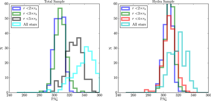
Figure 4. Plot of the PA0 distributions resulting from the 200 bootstrap/Monte Carlo runs with noise-added radial velocities. The left panel is for the total sample and the right panel is the Hydra-only sample. Differences in the number of stars and radii covered in each of these samples should be noted. The entire Hydra sample falls within  and the total combined sample extends out to
  . The all-stars histogram in the Hydra panel is therefore comparable to the
  histogram in the total combined panel on the left.
Download figure:
Standard image High-resolution imageIn Figure 5, we plot the amplitude and axis of rotation as a function of the max radius used to define each sample. The vertical error bars on each point represent the error in the fit parameters. The wide blue error bars on the top panel represent the standard deviation of the PA0 distributions resulting from the bootstrap/Monte Carlo analysis outlined in Section 3.2 and shown in Figure 4. The length of these error bars was equivalent when using the total combined sample or just the Hydra sample. For  , the standard deviations of the bootstrap distributions ranged from
  , and at larger radii they ranged from
  . Similar bootstrap error bars were not included on the Arot panel because they were equivalent to the error on the Arot fit (
 ).
).

Figure 5. Plot of the rotation-curve fit parameters determined using samples with different max radii rmax. The points mark the values listed in Table 2. The values determined using just the Hydra sample are shown as filled red circles and the values determined using the total sample are shown as empty circles. The thick blue error bars on the top panel represent the standard deviations of the PA0 distributions generated by our Monte Carlo technique.
Download figure:
Standard image High-resolution imageIn the bottom panel of Figure 5 we present a measure of the signal-to-noise ratio (S/N) of the strength of the rotation at each rmax value. We calculated this ratio by dividing  by the mean error on the
  values used in constructing the rotation curves. The mean error on
  was calculated as two times the standard deviation in
  as determined from our bootstrap analysis. At all radii, this value was
  . By calculating this S/N we are able to determine at which rmax values the internal rotation in the cluster is significant (S/N ≥ 1).
Figure 5 illustrates that there is a considerable change in the axis of rotation depending on the sample of stars being used. This characteristic suggests that assigning a global PA0 value for all stars at all radii in the cluster will not necessarily correspond to the strongest rotation signature. To further illustrate this point, we performed the rotation analysis on two subsets of the RV sample, one with all stars within 2rh, and another with all stars outside of 2rh. The rotation curves for each of these samples are shown in Figure 6. The number of stars, rotation amplitude, and axis of rotation for each sample are listed in Table 3. Figure 6 shows clearly that the rotation in the inner and outer regions of the cluster are defined by very different PAs, with the inner sample having  and the outer having
  (note that the direction of the angular momentum vectors of the inner and outer samples are, respectively, 126◦ and 266◦; see Figure 7). Interestingly, this analysis also illustrates that there is a signature of counter rotation between the inner and outer regions of M53 (see also Figure 8 below).

Figure 6. Left: plot of the rotation curve and fit resulting from using only those stars that fall within 2rh. Right: same as the left panel but using only stars that fall outside of 2rh. In each panel, the red line is the fit to the rotation curve with the sine function shown in Equation (1).
Download figure:
Standard image High-resolution image
Figure 7. Polar projection plot of the inner regions ( ) of M53. The dashed red circle marks 2rh. The axis of rotation defined by the total sample is shown by a dashed gray line, and the axis defined by the Hydra-only sample is shown by the solid gray line. The green arcs are the
  levels (
 ) of the
  PA0 bootstrap distributions shown in Figure 5. The stars on this plot are color coded according to the difference from the systemic velocity of the cluster, with red points being more positive and blue points being more negative. The size of the points is set by the absolute value of this difference (e.g., smaller points are closer to the systemic velocity and larger points are either more positive or more negative). The arrow indicates the direction of NGC 5053.
Download figure:
Standard image High-resolution image
Figure 8. Rotation profiles for the total ( ) and Hydra-only (
 ) sample. The error bars in the x direction are set to be the width of the bin (1
 25) used in constructing the rotation profile. The vertical error bars are the standard deviation of the RVs in a given bin. The dashed red line is a linear fit to the inner region of the rotation profile. The thick black lines are the rotation curves resulting from the fits to Equation (3).
Download figure:
Standard image High-resolution imageTable 3. Inner vs. Outer Rotation Parameters
| Sample | NTotal | Arot | PA0 |
|---|---|---|---|
( ) ) |
(deg) | ||
| (1) | (2) | (3) | (4) |
| Inner sample | 75 | 2.76 | 306.15 |
| Outer sample | 170 | 0.80 | 85.9 |
Download table as: ASCIITypeset image
We follow convention and use a single value for the PA0 defined by all stars at all radii in both the total sample and the Hydra-only sample, giving  and
and  , respectively. The implications of the change in PA0 will be further discussed in Section 5. In Figure 7, we present a polar representation of the positions of stars in our sample, their individual RV measurements, and where the stars fall relative to the axis of rotation.
4.2. Differential Rotation
The rotation-curve analysis clearly showed the signatures of differential rotation in the cluster, as illustrated in Figures 3 and 5 by the decrease in rotation amplitude with increasing radius. By constructing rotation profiles of the cluster, we can further illustrate and quantify the differential rotation in the cluster. We create overlapping bins along the axis that is perpendicular to the axis of rotation determined by fitting the rotation curves. We then calculate the difference between the average velocity in these cylindrical bins with the systemic velocity of the cluster. This results in a measurement of the rotation velocity of the cluster at different radii away from the axis of rotation. In Figure 8, we plot the rotation profiles of each sample using the PA0 determined by all of the stars in the total sample (318 65) and Hydra-only sample (
 ), respectively.
These rotation profiles show the strongest signature of rotation toward the cluster center. If we assume that the inner regions of the cluster follow solid-body rotation, we can model this portion of the rotation profile with a simple linear fit (y = mx). We only included the radial bins out to where the rotation profiles begin to turn over. For the total sample this position corresponded to  , and for the Hydra-only sample
  . The resulting linear fits are shown by a red dashed line in each panel of Figure 8. The slope of this line is
  for the total sample rotation profile, and
  for the Hydra-only sample. The rotational velocity given by this linear model at the turnover points listed above gives an estimate of the maximum rotational velocity in the cluster. By averaging the values of the linear model at the turnover points for each sample, we find the following rotational velocities:
  ,
, 
 . The rotational velocity for the Hydra sample is consistent with the values determined from the rotation-curve analysis presented in Figure 3. It is interesting that both rotation profiles do not converge to 0
  at large perpendicular distances from the axis of rotation. This feature might be another manifestation and consequence of the decoupling between the inner and outer rotation already suggested by the radial variation of the rotation axis. Additional data probing the kinematics of the outermost region would be necessary to further explore the significance of this feature.
We also performed an additional fit of the rotation profile using the following simple analytical model (as in, e.g., Lynden-Bell 1967; Hénault-Brunet et al. 2012; Mackey et al. 2013; Kacharov et al. 2014):

In this equation, vrot is the rotational velocity at a distance r from the cluster center measured perpendicularly from the axis of rotation, Apeak is the maximum amplitude of the rotational velocity, and rpeak is the distance from the rotation axis where vrot reaches the maximum value, Apeak.
When performing this fit we only included the bins between  away from the axis of rotation. This resulted in the following values for the different samples:
  ,
,  Apeak(Hydra) =
  , rpeak(Hydra) =
  . The peak of the rotation curve, located approximately at the cluster half-light radius, is in general agreement with the simulations presented in Vesperini et al. (2014), Tiongco et al. (2017), and M. A. Tiongco et al. (2017, in preparation).
4.3. Velocity Dispersion Profile
The total combined sample has extensive radial coverage in both the inner and outer regions of M53, allowing us to construct a velocity dispersion profile of the cluster. To do so, the sample was divided into six radial bins with approximately the same number of stars. The final bin was split in half an additional time because it covered such a large range in radii. In the top panel of Figure 9, we plot the RV of each star as a function of its radius in arcminutes. Along the top of this panel, we also show the radial extent of each sample as wide horizontal bars. The black diamond within each bar marks the median radial distance of each sample. The solid vertical lines mark the inner and outer radius limit of each bin. Within each bin, we use the maximum likelihood method described in Section 3.1 to get an estimate of the mean velocity and velocity dispersion ( ). This produces a measurement of the velocity dispersion as a function of radius, as shown in the bottom panel of Figure 9. The radius for each point in this panel marks the mean of the radii in a given bin. We fit a Plummer model (Plummer 1911) to the profile in the bottom panel of Figure 9 in order to get an estimate of the central velocity dispersion in the cluster. This was done using Equation (4) with the central velocity dispersion,
  , and scale radius, rs, being the free parameters:


Figure 9. Top: plot of the radial velocities of the individual stars as a function of their distance from the cluster center in arcminutes. The solid blue line marks the mean RV of the entire sample. The thick horizontal lines extending across each bin are the 3σ levels of radial velocity sample in that bin. Stars that fell outside of these levels were not included in the velocity dispersion calculations and are marked as red "x". Bottom: velocity dispersion as a function of radial distance from the cluster center. The number at the bottom of each bin indicates the number of stars it contains. The solid black line is the best-fit Plummer model to the dispersion profile. The best-fit central velocity dispersion and Plummer scale length are shown in the plot. The dashed black line shows the Plummer fit where rs was fixed to equal rh.
Download figure:
Standard image High-resolution imageThe resulting fit is shown as a solid black line in the bottom panel of Figure 9. From this fit, we find 
 and
and  (
( , assuming RSun = 17.9 kpc). These values are consistent with Lane et al. (2009) who found
 and
and  . We performed an additional fit to the velocity dispersion profile using a Plummer model with the scale radius (rs) fixed to the projected half-light radius (
 ). The result of this fit is shown as the dashed line in the bottom panel. This fit was calculated to test how well the Plummer model describes the dispersion profile given that it is expected that the scale radius is equivalent to the projected half-light radius (see Haghi et al. 2009; Lane et al. 2010b; Kacharov et al. 2014). The fit with a fixed scale radius produced a higher central velocity dispersion
 , although it does not fit the dispersion profile as well as the Plummer model where
  and rs are both free parameters. Although the Plummer model provides a convenient analytical model to determine the central velocity dispersion, this discrepancy clearly suggests that a complete characterization of all the dynamical properties of this cluster will require more sophisticated numerical or analytical models. Some of the peculiar dynamical features found in this study already provide a clear indication of the degree of dynamical complexity of this cluster.
5. Discussion and Conclusions
Our analysis of the kinematics of M53 has clearly shown that the inner regions of M53 exhibit a significant amount of internal rotation and revealed the presence of a radial gradient of the PA of the rotation axis (see also Bianchini et al. (2013) for a study revealing a similar radial gradient in the PA of the rotation axis in 47 Tuc and M15). Such a radial gradient suggests a decoupling between the cluster inner rotation imprinted by the cluster formation and early dynamics and that of the outer region which might instead be affected by the interaction of the cluster with the Milky Way tidal field (and, possibly, with the nearby cluster NGC 5053).
To illustrate this point, we show in Figure 10 the analysis of a snapshot of an N-body simulation of a rotating cluster starting with an inner rotation following the models introduced by Varri & Bertin (2012) and assuming a rotation axis lying on the cluster orbital plane around the center of the host galaxy combined with a solid-body rotation around an axis perpendicular to the orbital plane and initially synchronous with the cluster orbital motion. As the cluster evolves, angular momentum redistribution inside the cluster and loss through escaping stars result in the evolution of the initial rotational profile. A complete discussion of the dynamics of this and other models will be presented elsewhere M. A. Tiongco et al. (2017, in preparation) but here, in Figure 10, we show the analysis of a typical snapshot of our simulations. The top panel shows the radial variation of the angle between the total angular momentum in different spherical shells and an axis perpendicular to the cluster orbital plane as a function of the distance of the shell from the cluster center; in the bottom panel, we present the cumulative radial variation of the PA determined following the procedure used for the analysis of the observational data. We point out that the N-body simulation is not meant to provide a detailed model for M53; this figure serves to illustrate how complex structural and kinematical properties might lie behind the modest PA radial gradient found in the observational data. Velocity measurements for a larger sample of stars would be needed to carry out an observational study of the PA radial gradient in differential shells and further explore its strength and statistical significance.

Figure 10. Analysis of a snapshot of a rotating cluster N-body simulation (see Section 5) Top panel: radial gradient of the angle  between the angular momentum of stars within differential 3D spherical shells at distance r (normalized to the 3D half-mass radius rh) from the cluster center and an axis perpendicular to the cluster orbital plane around its host galaxy. Bottom panel: radial variation of the PA in cumulative radial shells calculated using the procedure followed for the analysis of observational data. The points (error bars) in this panel show the mean (error on the mean) of the PA for each shell calculated from 300 samples each containing 300 stars.
Download figure:
Standard image High-resolution imageOur various estimates of Vrot and the central velocity dispersion  determined using a Plummer model give us insight into how the internal rotation in M53 is affecting its morphological features. This is typically done by plotting the ratio
  as a function of the ellipticity
  of the cluster. In Figure 11, we plot this relationship for M53, and a sample of GCs taken from Fabricius et al. (2014) and Bellazzini et al. (2012). The data taken from Fabricius et al. (2014) are plotted as (
 . The product of the velocity gradient (
 ) and the cluster half-light radius (rh) is equivalent to the Vrot values determined using individual RVs as done in this study. Bellazzini et al. (2012) adopted the Arot values (instead of Arot/2) as a measure of the peak rotation amplitude to account for radial variation in the rotational velocity. We mention this to place our M53 results in the context of the different ways rotation velocities are reported in the literature.

Figure 11. Ratio of the rotation velocity Vrot to the central velocity dispersion  vs. ellipticity for a sample of GCs taken from Bellazzini et al. (2012) and Fabricius et al. (2014). The filled circle is the ratio value for M53 as found by Fabricius et al. (2014). Our results for M53 are included in this plot as green markers that correspond to our different estimates of Vrot. The filled square and triangle correspond to
  , respectively, as determined by fitting the analytical differential rotation model (Equation (3)) to the rotation profiles described in Section 4.2. The open square corresponds to
  , as determined from the maximum rotation amplitude from the rotation-curve analysis shown in Figure 3. For all of the M53 data points, we assumed
  , as determined from the Plummer model fit to the velocity dispersion where the scale radius was a free parameter. The blue curve marks the
  as defined for isotropic spherical rotators.
Download figure:
Standard image High-resolution imageFigure 11 also includes a simple model of isotropic oblate rotators (Kormendy 1982) assuming  (i.e., not corrected for inclination). All of our estimates of Vrot in M53 put it above this model. It is not surprising, however, that M53 shows deviations from the expected behavior of an isotropic oblate rotator. The emerging complexity of the velocity space of M53, as evidenced by the radial gradient in its axis of rotation, goes well beyond the stringent hypothesis of an isotropic oblate rotator. In addition, the only measurement currently available for M53 in the literature relies on the early study by White & Shawl (1987), as reported in the Harris catalog. Such an analysis was based on photographic plates and the bright limiting magnitude of their data did not allow them to measure the ellipticity at large cluster radii, making their measurements constrained to the inner regions of the clusters. It should also be noted that the few clusters for which a more detailed morphological study has been carried out (see Bianchini et al. (2013) and references therein) revealed a radial variation of the ellipticity and showed that more sophisticated dynamical models are necessary to describe their complex kinematical and morphological properties. This should be taken as further motivation to perform a complete characterization on the morphology of M53. Similarly to M53, the majority of the Fabricius et al. (2014) measurements, which also represent the maximum rotation velocities at small radii, fall on or above the isotropic rotator model. The Bellazzini et al. (2012) measurements (adopting Arot to account for the radial variation of Vrot) populate both the region above and below this curve. These differences further highlight the importance of using caution in the interpretation of this plot to draw conclusions concerning the role of different kinematical ingredients in determining a cluster morphology.
Bellazzini et al. (2012) found a relatively strong correlation between the cluster metallicity and  . It should be noted, however, that Kimmig et al. (2015) did not find a similar correlation. In Figure 12, we plot [Fe/H] as a function of
  for the Bellazzini et al. (2012) sample and the values determined for M53 in this study. Here we see that M53 follows the correlation found by Bellazzini et al. (2012) when
  is calculated from the differential rotation profile of the entire sample. The
  values determined from the Hydra-only sample and peak rotation amplitude of the inner cluster (
 ), however, deviate from the trend set by the other GCs shown in the figure. The locations of the different M53 measurements relative to this trend further highlight the impact of measuring cluster rotation over different radial ranges.

Figure 12. Cluster metallicity as a function of  for the Bellazzini et al. (2012) sample. Our values for M53 are shown as green markers whose shapes correspond to the different Vrot estimates as given in the caption of Figure 11.
Download figure:
Standard image High-resolution image
Lane et al. (2009) and Kimmig et al. (2015) also both produced measurements of the rotation in M53 using methods similar to what we have presented here. Lane et al. (2009) concluded that there was no rotation above  , and Kimmig et al. (2015) found a similar value of
  . Our analysis of the total combined sample leads to a similar conclusion as shown by the values at the bottom of Table 2 and final panels in Figure 3. Neither of these studies provided a measurement of the rotation axis given that the amplitude of rotation was found to be insignificant. What we have gained through this study, that was not possible with Lane et al. (2009) and Kimmig et al. (2015), is a detailed look at the inner (
 ) cluster regions, which clearly show a strong signature of internal rotation. Our results from this inner region are in agreement with the amount of rotation detected by the Fabricius et al. (2014) IFU study. Although that study focused on the very central regions of M53
  , they found
  , which is equivalent to what we measure when deriving Vrot from the amplitude of the rotation curves.
The results of our study show that M53 clearly exhibits strong internal rotation in its central regions with a complex radial profile, characterized by a differential distribution of the angular momentum as well as a radial variation of the PA of the principal axis of rotation. In the presence of such rich internal kinematics, a detailed morphological analysis by means of deep wide-field photometry over the entire radial extent of the cluster is essential in order to provide a complete interpretative picture of the dynamical properties of this unique object. The data currently available in the literature are too limited to allow such a characterization, which has motivated the next step in our comprehensive analysis of this cluster system. The photometry we have already collected will also allow us to investigate the structural properties of the outskirts and to identify possible morphological features resulting from the perturbations induced by the external tidal field, such as tails or bridges.
The observational results we presented here will be of crucial importance to enrich the traditional picture of the long-term evolution of collisional stellar systems, especially regarding the study of the largely unexplored interplay between internal rotation and external tidal field (see Tiongco et al. 2016, 2017, and M. A. Tiongco et al. 2017, in preparation).
We would like to thank the referee for their detailed report and insightful suggestions that expanded and improved the analysis in our study.
Footnotes
- 3
The WIYN Observatory is a joint facility of the University of Wisconsin-Madison, Indiana University, the National Optical Astronomy Observatory, and the University of Missouri.