


Abstract
We model the long-term X-ray and ultraviolet (XUV) luminosity of TRAPPIST-1 to constrain the evolving high-energy radiation environment experienced by its planetary system. Using a Markov Chain Monte Carlo (MCMC) method, we derive probabilistic constraints for TRAPPIST-1's stellar and XUV evolution that account for observational uncertainties, degeneracies between model parameters, and empirical data of low-mass stars. We constrain TRAPPIST-1's mass to m⋆ = 0.089 ± 0.001 M⊙ and find that its early XUV luminosity likely saturated at  . From the posterior distribution, we infer that there is a ∼40% chance that TRAPPIST-1 is still in the saturated phase today, suggesting that TRAPPIST-1 has maintained high activity and LXUV/Lbol ≈ 10−3 for several gigayears. TRAPPIST-1's planetary system therefore likely experienced a persistent and extreme XUV flux environment, potentially driving significant atmospheric erosion and volatile loss. The inner planets likely received XUV fluxes ∼103–104 times that of the modern Earth during TRAPPIST-1's ∼1 Gyr long pre-main-sequence phase. Deriving these constraints via MCMC is computationally nontrivial, so scaling our methods to constrain the XUV evolution of a larger number of M dwarfs that harbor terrestrial exoplanets would incur significant computational expenses. We demonstrate that approxposterior, an open source Python machine learning package for approximate Bayesian inference using Gaussian processes, accurately and efficiently replicates our analysis using 980 times less computational time and 1330 times fewer simulations than MCMC sampling using emcee. We find that approxposterior derives constraints with mean errors on the best-fit values and 1σ uncertainties of 0.61% and 5.5%, respectively, relative to emcee.
Export citation and abstract BibTeX RIS
1. Introduction
The James Webb Space Telescope (JWST) is poised to detect and characterize the first terrestrial exoplanet atmospheres via transmission spectroscopy. This search will likely focus on planets orbiting nearby M dwarfs given their favorable relative transit depths, the potential buildup of biosignature gases due to ultraviolet-driven photochemistry (Segura et al. 2005), and the large occurrence rates of M dwarf planets (Dressing & Charbonneau 2015). The correct interpretation of those observations, however, is predicated on understanding the system's long-term evolution, most importantly processes that could affect the planet's atmospheric state and habitability, such as atmospheric escape, water loss, and the potential buildup of an abiotic O2 atmosphere (Watson et al. 1981; Lammer et al. 2003; Murray-Clay et al. 2009; Luger & Barnes 2015). These volatile escape mechanisms are partially driven by the host star's XUV luminosity (X-ray and extreme ultraviolet emission ranging over approximately 1–1000 Å), and therefore characterizing the long-term stellar XUV evolution of late M dwarfs is critical to assessing the present state of their planets, including habitability.
High-energy stellar radiation originates from the corona via the heating of magnetically confined plasma (Vaiana et al. 1981). The stellar magnetic field is likely generated via differential rotation within the stellar convective envelope (Parker 1955), linking rotation to stellar activity and XUV emission. Stellar rotation rates slow over time because of magnetic braking (Skumanich 1972), causing XUV emission to decline with time. The X-ray luminosity (LX) of FGK stars, for example, has been empirically shown to monotonically decrease with age (Jackson et al. 2012). This trend has also been observed for commonly used proxies for stellar age, rotation period, and Rossby number (Ro = Prot/τ for convective turnover timescale τ; Pizzolato et al. 2003; Wright et al. 2011).
Stellar activity evolution is characterized by two distinct phases. First, in the saturated phase, young, rapidly rotating stars (Ro ≲ 0.1) maintain a constant LX/Lbol ≈ 10−3 (Wright et al. 2011; Jackson et al. 2012). Then, at longer rotation periods and larger Ro, stars transition to the unsaturated phase in which LX/Lbol exponentially decays over time (Pizzolato et al. 2003; Ribas et al. 2005). Recent work has shown that the stellar dynamo processes that generate magnetic fields and drive XUV emission in fully convective M dwarfs follow the same evolution with Ro as described above for solar-type stars (Wright & Drake 2016; Wright et al. 2018). We can therefore apply this model to examine the XUV evolution of individual fully convective stars.
TRAPPIST-1 (Gillon et al. 2016, 2017), an ultracool dwarf located 12 pc from Earth, harbors seven approximately Earth-sized transiting planets that are prime targets for JWST transmission spectroscopy observations (Morley et al. 2017; Lincowski et al. 2018; Lustig-Yaeger et al. 2019). TRAPPIST-1's high observed LX (Wheatley et al. 2017), short photometric rotation period (3.3 days, Luger et al. 2017), and low Rossby number (Ro ≈ 0.01, Roettenbacher & Kane 2017) suggest that TRAPPIST-1 is still saturated today (Pizzolato et al. 2003; Wright et al. 2011, 2018). Both Roettenbacher & Kane (2017) and Morris et al. (2018) suggest that the photometrically determined rotation period is inaccurate, with the latter study proposing that the 3.3 day period corresponds to a characteristic timescale for active regions on the stellar surface. TRAPPIST-1's v sini = 6 km s−1 (Barnes et al. 2014), however, implies a rotation period of ∼1 day for i = 90°, providing evidence that TRAPPIST-1's rapid rotation is physical and consistent with saturation (Prot ≲ 20 days, Wright et al. 2018).
The TRAPPIST-1 planetary system currently receives significant high-energy fluxes (Bourrier et al. 2017b; Wheatley et al. 2017; Peacock et al. 2019), possibly a consequence of TRAPPIST-1 remaining in the saturated regime. These fluxes were likely more extreme during the pre-main-sequence, driving significant water loss and potentially rendering the planets uninhabitable (Bolmont et al. 2017; Bourrier et al. 2017a). Here, we model the long-term stellar and XUV evolution of TRAPPIST-1 to characterize the evolving XUV environment of its planetary system. We use a Markov Chain Monte Carlo (MCMC) method to derive probability distributions for our model parameters that describe the XUV evolution that are consistent with TRAPPIST-1's observed properties and their uncertainties.
TRAPPIST-1 is not the only system that merits this modeling, however, as the Transiting Exoplanet Survey Satellite will likely discover additional transiting planets orbiting in the habitable zone of nearby M dwarfs (Barclay et al. 2018), some of which may be suitable targets for atmospheric characterization with JWST. In this work, we show that stellar XUV histories can be accurately inferred using machine learning (approxposterior, Fleming & VanderPlas 2018), but using 980 times less computational resources than traditional MCMC methods. This speed-up enables our methods to scale to additional stars that host potential targets for atmospheric characterization and is generalizable to a large number of applications, potentially enabling Bayesian statistical analyses that are otherwise intractable with traditional MCMC approaches, such as emcee (Foreman-Mackey et al. 2013).
We describe our model and statistical methods in Section 2. We present our results and demonstrate the ability of machine learning to reproduce our analysis in Appendix 3, and we discuss the implications of our results in Section 4. In Appendix A, we describe the approxposterior algorithm and discuss its convergence properties.
2. Methods
2.1. Simulating XUV Evolution with VPLanet
We simulate TRAPPIST-1's stellar evolution using the STELLAR module in VPLanet6 (Barnes et al. 2020), which performs a bicubic interpolation over mass and age of the Baraffe et al. (2015) stellar evolution tracks. The Baraffe et al. (2015) models (also employed by both Burgasser & Mamajek 2017 and Van Grootel et al. 2018 to constrain TRAPPIST-1's stellar properties) were computed for solar-metallicity stars and hence are suitable for TRAPPIST-1, whose [Fe/H] is consistent with solar (Gillon et al. 2016; see also Burgasser & Mamajek 2017).
We assume TRAPPIST-1's LXUV evolution traces that of LX and use the Ribas et al. (2005) model,

where fsat is the constant ratio of stellar XUV to bolometric luminosity during the saturated phase, tsat is the duration of the saturated phase, and βXUV is the exponent that controls how steeply LXUV decays after saturation.
Note that each VPLanet simulation (and hence likelihood calculation, see Section 2.4) in principle only requires interpolating the Baraffe et al. (2015) Lbol tracks and evaluating an explicit function of time to compute LXUV, both computationally cheap tasks. VPLanet, however, is a general-purpose code designed to simulate the evolution of an exoplanetary system and its host star by simultaneously integrating coupled ordinary differential equations and explicit functions of time that describe the evolution. This generalized structure requires numerous steps to facilitate physical couplings, such as validation steps and a host of intermediate calculations (for more details, see Barnes et al. 2020). Moreover, STELLAR simultaneously evolves a star's radius, effective temperature, radius of gyration, LXUV, and rotation rate in addition to Lbol, adding computational overhead. Each VPLanet simulation using STELLAR lasts about 10 s.
2.2. Markov Chain Monte Carlo Analysis
We use emcee, a Python implementation of the affine-invariant Metropolis–Hastings MCMC sampling algorithm (Foreman-Mackey et al. 2013), to infer posterior probability distributions for our model parameters that describe the evolution of TRAPPIST-1. These distributions are conditioned on observations of TRAPPIST-1 and the activity evolution of late-type stars, and they account for both observational uncertainties and correlations between parameters. Our model parameters that we fit for via MCMC comprise the state vector

where m⋆ and age are the stellar mass and age, respectively, and the other parameters are defined by Equation (1). All of the code used to perform the simulations and analysis in this work is publicly available online.7
2.3. Prior Probability Distributions
Since we have few available observable properties of TRAPPIST-1 to use to condition our analysis (Lbol and LXUV/Lbol; see Section 2.4), our prior probability distributions will strongly impact our results. We use previous studies and empirical data of late M dwarfs to assemble the best available constraints to serve as priors for our MCMC analysis. We list our adopted prior probability distributions in Table 1.
Table 1. Prior Distributions
| Parameter (units) | Prior | Notes |
|---|---|---|
| m⋆ (M⊙) |

|
⋯ |
| fsat |

|
Wright et al. (2011) |
| tsat (Gyr) |

|
⋯ |
| Age (Gyr) |

|
Burgasser & Mamajek (2017) |
| βXUV |

|
Jackson et al. (2012) |
Download table as: ASCIITypeset image
Following Van Grootel et al. (2018), we rely on TRAPPIST-1's luminosity and age to constrain its mass. We therefore adopt a simple uniform prior of  M⊙. For the age, we use the empirical estimate for TRAPPIST-1 derived by Burgasser & Mamajek (2017), age
  Gyr, as their thorough analysis considered both observations of TRAPPIST-1 and a host of empirical age indicators for ultracool dwarfs. This age distribution is consistent with Gonzales et al. (2019), who conclude that TRAPPIST-1 is a field-age dwarf based on their spectral energy distribution modeling. We cap the maximum age we consider at 12 Gyr. Younger ages have been suggested based on TRAPPIST-1's activity (e.g., ≳500 Myr, Bourrier et al. 2017b), but here we argue that the behavior is consistent with an extended saturation timescale.
We construct an empirical  distribution from the sample of fully convective, saturated M dwarfs with observed LX from Wright et al. (2011). For each star in the Wright et al. (2011) sample, we follow Wheatley et al. (2017) and estimate LXUV as a function of LX using Equation (2) from Chadney et al. (2015). We find that the distribution is well approximated by a normal distribution,
  , and we adopt it as our prior.
The duration of the saturated phase is estimated to be tsat ≈ 100 Myr for FGK stars (Jackson et al. 2012). Studies of stellar activity of late-type stars as a function of stellar age, or its proxy rotation period, indicate that the activity lifetime, and hence duration of the saturated phase, is likely longer for later-type stars (Wright et al. 2011; Shkolnik & Barman 2014; West et al. 2015), with fully convective M dwarfs potentially remaining active throughout their lifetimes (tsat ≳ 7 Gyr, West et al. 2008; Schneider & Shkolnik 2018). Furthermore, the spin-down timescales of late M dwarfs increase with decreasing stellar mass (Delfosse et al. 1998), with late M dwarfs retaining rapid rotation longer than earlier-type stars and hence remaining active for up to Prot ≈ 86 days (West et al. 2015), much longer than TRAPPIST-1's estimated rotation period. Given these constraints, we adopt a broad uniform tsat prior distribution capped by the maximum age we consider,  Gyr.
Gyr.
In the unsaturated phase, LX, and hence LXUV, decay exponentially with power-law slope βXUV (Ribas et al. 2005). Jackson et al. (2012) find that βXUV does not significantly vary with stellar mass in their sample of FGK stars. Since Wright & Drake (2016) found that the X-ray evolution of fully convective stars is qualitatively similar to that of partially convective FGK stars, we adopt the βXUV distribution of late K dwarfs from the Jackson et al. (2012) sample as our prior,  .
.
2.4. Likelihood Function and Convergence
We further condition our analysis on TRAPPIST-1's observed bolometric luminosity,  (Van Grootel et al. 2018, but see also Gonzales et al. 2019), and LXUV/Lbol = 7.5 ± 1.5 × 10⁻⁴ (Wheatley et al. 2017). In other words, we require that our forward models (VPLanet simulations) yield results that are consistent with the observations of TRAPPIST-1 and their uncertainties.
For a given state vector  , we define the natural logarithm of our likelihood function,
  , as
, as
where Lbol, LXUV/Lbol and Lbol( ), LXUV/Lbol(
 ) are the observed values and VPLanet outputs given
  , respectively, and
  and
and  are the observational uncertainties. For each
  , we compute the natural logarithm of the posterior probability at
  , or "lnprobability," required for ensemble MCMC sampling as
  . We use the distributions described in Section 2.3 to calculate the natural logarithm of the prior probability of
  ,
,  .
.
We run our MCMC with 100 parallel chains for 10,000 iterations, initializing each chain by randomly sampling each element of  from their respective prior distributions. During each step of the MCMC chain, VPLanet takes
  as input and simulates TRAPPIST-1's evolution up to the age in
  , predicting Lbol and LXUV/Lbol to evaluate
  . We discard the first 500 iterations as burn-in and assess the convergence of our MCMC chains by computing the integrated autocorrelation length and acceptance fraction for each chain. We find a mean acceptance fraction of 0.48 and a minimum and mean number of iterations per integrated autocorrelation length of 93 and 132, respectively, indicating that our chains have converged (Foreman-Mackey et al. 2013). Given our integrated autocorrelation lengths, our MCMC chain yielded about 10,000 effective samples from the posterior distribution.
2.5. Inference with approxposterior
The methods presented above can be applied to any late-type star to constrain its LXUV history, given suitable priors and observational constraints. Our MCMC analysis, however, required 4070 core hours on the University of Washington's Hyak supercomputer to converge. The main computational cost is incurred by running a ∼10 s VPLanet simulation each MCMC step to evaluate  , requiring ∼1,000,000 simulations in total for the full MCMC analysis. Assuming similar convergence properties, repeating this analysis for even a modest sample of 30 stars would require ∼122,000 core hours, a significant computational expense. Moreover, performing a similar analysis with a more computationally expensive model would only exacerbate this issue.
To mitigate the computational cost, we apply approxposterior,8 an open source Python machine learning package (Fleming & VanderPlas 2018), to compute an accurate approximation to the true MCMC-derived posterior distribution for TRAPPIST-1's XUV evolution. approxposterior, a modified implementation of the "Bayesian Active Learning for Posterior Estimation" (BAPE) algorithm of Kandasamy et al. (2017), trains a Gaussian process (GP; see Rasmussen & Williams 2006) replacement for the lnprobability evaluation, learning on the results of VPLanet simulations. The GP is then used within an MCMC sampling algorithm, such as emcee, to quickly obtain the posterior distribution. In our case, predicting the lnprobability using the GP (∼130 μs) is 80,000 times faster than running VPLanet (10 s) for each lnprobability evaluation, yielding a massive reduction in computational cost.
Following Kandasamy et al. (2017), approxposterior iteratively improves the GP's predictive ability by identifying high-likelihood regions in parameter space, and hence high-posterior-density regions, where the GP predictions are uncertain. approxposterior then evaluates VPLanet in those regions to supplement the training set, improving the GP's predictive ability in the relevant regions of parameter space, while minimizing the number of forward-model evaluations required for suitable predictive accuracy. Similar techniques using a GP surrogate model have been shown to rapidly and accurately infer Bayesian posterior distributions for computationally expensive cosmology studies (e.g., Bird et al. 2019; McClintock & Rozo 2019).
To model the covariance between points in the GP training set, we use a squared exponential kernel,

where xi and xj are two arbitrary points in parameter space and l is a hyperparameter that controls the scale length of the correlations. We assume correlations in each dimension have different scale lengths and fit for each l by optimizing the GP's marginal likelihood of the training set data using Powell's method (Powell 1964), randomly restarting this optimization 10 times to mitigate the influence of local extrema. To ensure our solution is numerically stable, we add a small white-noise term of  to the diagonal of the GP covariance matrix.
We initially trained the GP on a set of 50 VPLanet simulations with initial conditions sampled from our prior distributions. We then ran approxposterior until it converged after seven iterations. For each iteration, approxposterior selected 100 new training points according to the Kandasamy et al. (2017) point selection criterion. approxposterior ran VPLanet at each point for a total of 750 training samples. The trained GP was then used within emcee to quickly obtain the approximate posterior distribution following the same MCMC sampling procedure described above. In Appendix A, we provide additional information about the approxposterior algorithm and its convergence properties.
3. Results
3.1. The Evolution of TRAPPIST-1
In Figure 1, we display the posterior probability distributions for our model parameters derived using MCMC with VPLanet and emcee. We adopt the median values of the marginal distributions as our best-fit solutions and derive the lower and upper uncertainties using the 16th and 84th percentiles, respectively. We list these values in Table 2.

Figure 1. Updated joint and marginal posterior probability distributions for the TRAPPIST-1 stellar parameters given in Equation (2) made using corner (Foreman-Mackey 2016). The black vertical dashed lines on the marginal distributions indicate the median values and lower and upper uncertainties from the 16th and 84th percentiles, respectively. The blue curves superimposed on the marginal distributions display the adopted prior probability distribution for each parameter. From the posterior, we infer that there is a 40% chance that TRAPPIST-1 is still in the saturated phase today.
Download figure:
Standard image High-resolution imageTable 2. Updated Parameter Constraints and Errors
| Parameter (units) | VPLanet-emcee MCMC | approxposterior MCMC | approxposterior Relative Error | Monte Carlo Error |
|---|---|---|---|---|
| m⋆ (M⊙) |

|

|

|
3.41 × 10⁻⁶ |
| fsat |

|

|
<0.1% | 1.23 × 10⁻³ |
| tsat (Gyr) |

|

|
1.81% | 2.0 × 10⁻² |
| Age (Gyr) |

|

|
1.47% | 1.30 × 10⁻³ |

|

|

|
0.86% | 2.12 × 10⁻³ |
| P(saturated) | 0.40 | 0.39 | 2.5% | 3.30 × 10⁻³ |
Note. Best-fit values and uncertainties are derived using the medians and 16th and 84th percentiles from the marginal posterior distributions, respectively. P(saturated) indicates the posterior probability that TRAPPIST-1 is still in the saturated regime today. The relative errors are computed as the absolute percent difference between the best-fit values derived by emcee and approxposterior. The approxposterior-derived results are in good agreement with the fiducial emcee MCMC.
Download table as: ASCIITypeset image
TRAPPIST-1 likely maintained a large LXUV throughout its lifetime as we find  and
and  Gyr, consistent with the observed LXUV/Lbol and long activity lifetimes of late M dwarfs (West et al. 2008; Wright et al. 2018). The long upper tail in the marginal fsat distribution arises from the combination of the degeneracy between fsat and tsat and from our strong empirical fsat prior that disfavors fsat ≳ −2.5. The degeneracy stems from our model attempting to match TRAPPIST-1's observed LXUV/Lbol. For example, larger values of fsat produce high initial LXUV/Lbol, requiring shorter tsat, and hence an earlier transition to unsaturated LXUV/Lbol decay, to decrease LXUV/Lbol to its observed value, and vice versa.
Although our tsat prior distribution, based on empirical measurements of late M dwarfs (see Section 2.3), equally favors both short and long saturation timescales, the marginal posterior density for tsat steeply declines for tsat ≲ 4 Gyr. This decline implies that ultracool dwarfs like TRAPPIST-1 likely remain saturated for many gigayears. Our analysis strongly disfavors short saturation timescales, with only a 0.5% chance that tsat ≤ 1 Gyr, the saturation timescale adopted by Luger & Barnes (2015) in their analysis of water loss from exoplanets orbiting in the habitable zone of late M dwarfs and in Lincowski et al. (2018). From the posterior distribution, we infer that there is a 40% chance that TRAPPIST-1 is still in the high-LXUV/Lbol saturated phase today, suggesting that the TRAPPIST-1 planets could have undergone prolonged volatile loss.
The marginal age and βXUV posterior distributions reflect their prior distributions as for the former, and Lbol is not sufficient to constrain TRAPPIST-1's age beyond our adopted prior because the luminosities of ultracool dwarfs do not significantly change during the main sequence (Baraffe et al. 2015). The marginal posterior for βXUV does not vary from the prior because our XUV model is overparameterized with three parameters to fit two observations, although all are motivated by empirical data and hence merit inclusion. Our model prefers to exploit the degeneracy between fsat and tsat to match TRAPPIST-1's observed LXUV in our MCMC instead of varying the slope of the unsaturated LXUV decay. Even though our model is overparameterized, the observations of TRAPPIST-1 used to condition our probabilistic model do in fact influence the posterior distribution because the reduction in posterior variance relative to the prior can be seen in the joint posterior and marginal distributions of Figure 1 for m⋆, fsat, and tsat.
In the joint posterior distribution, age and βXUV weakly correlate with fsat, requiring a narrow spread of fsat ≈ −3.05 for young ages and steeper βXUV, respectively. Note that βXUV and tsat are uncorrelated, except at short tsat, where steep βXUV values are disfavored as this evolution would underpredict the observed LXUV. We constrain TRAPPIST-1's mass to m⋆ = 0.089 ± 0.001 M⊙, in good agreement with and six times more precise than the value derived by Van Grootel et al. (2018). In Section 3.3, we consider how this mass constraint affects TRAPPIST-1's predicted radius.
Finally, we estimate the Monte Carlo standard error (MCSE) for each model parameter. The MCSE does not reflect the inherent probabilistic uncertainty in our model that arises from conditioning on data with uncertainties, but rather it approximates the error incurred by estimating parameters using an ensemble of MCMC chains of finite length. Using the batch means method (Flegal et al. 2008; Flegal & Jones 2010), we find MCSEs for m⋆, fsat, tsat, age, and βXUV of 3.41 × 10⁻⁶, 1.23 × 10⁻³, 2.0 × 10⁻², 1.30 × 10⁻², and 2.12 × 10⁻³, respectively. These errors are much less than the posterior uncertainty and can be safely ignored.
3.2. Comparison with approxposterior
We compare the approximate posterior distribution derived using approxposterior with our previous results (referred to as the fiducial MCMC). We display the approximate joint and marginal posterior distributions in Figure 2 and list the marginal constraints derived by both methods in Table 2.
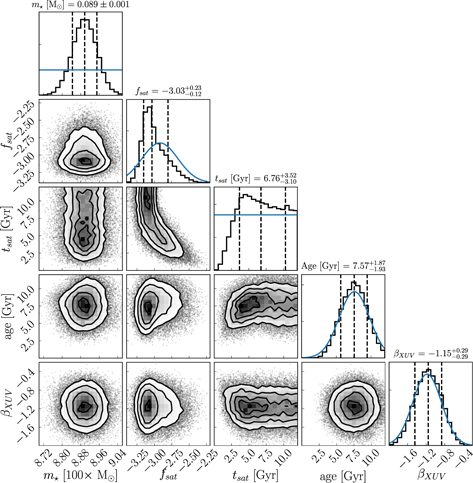
Figure 2. Same format as Figure 1, but derived by approxposterior. approxposterior-recovered constraints and parameter correlations are in good agreement with the emcee MCMC, but require 980 times less computational resources.
Download figure:
Standard image High-resolution imageAs seen in Figure 2, approxposterior recovers the nontrivial correlations between model parameters seen in the fiducial MCMC posterior distribution. We emphasize this good agreement by overplotting the approxposterior estimated posterior distribution (blue) on top of the fiducial MCMC results (black) in Figure 3.

Figure 3. New figure: same format as Figure 1, but with the fiducial posterior distribution in black and the approxposterior-derived posterior distribution in blue. The joint and marginal posterior distributions estimated by approxposterior are in excellent agreement with our fiducial emcee-derived results.
Download figure:
Standard image High-resolution imageOur parameter constraints derived using approxposterior are in good agreement with those inferred using emcee. We find average errors in parameter medians and 1σ uncertainties of 0.61% and 5.5%, respectively, relative to the constraints derived using emcee. These differences are larger than the MCSEs because the GP employed by approxposterior is an accurate, yet imperfect, surrogate for the lnprobability calculation. approxposterior tends to underestimate parameter uncertainties by a few percent because its algorithm preferentially selects high-likelihood points to expand its training set (see Appendix A.1). This concentration of high-likelihood points slightly biases the inferred GP scale lengths, l, toward smaller values, effectively overfitting. The smaller values of l shrink the estimated posterior distribution, producing the underestimated parameter uncertainties. We mitigate this effect by adding a small white-noise term to the diagonal of the GP covariance matrix.
Not only can approxposterior accurately recover Bayesian parameter constraints and correlations, but it does so extremely quickly. approxposterior requires only about 4 core hours to estimate the approximate posterior distribution, a factor of 980 times faster than our fiducial MCMC. Moreover, approxposterior used 1330 times fewer VPLanet simulations to build its training set than the ∼106 simulations ran by the fiducial MCMC for likelihood evaluations. This reduction in computational expense arises from a combination of approxposterior's GP-based lnprobability predictions only taking ∼130 μs, compared to the much longer 10 s per VPLanet simulation, and its intelligent iterative training set augmentation algorithm. approxposterior's efficient selection of the GP's training set focuses on high-likelihood regions to improve the GP's predictive ability in relevant regions of parameter space while minimizing the training set size.
Our findings demonstrate that approxposterior can be used to estimate accurate approximations to the posterior probability distributions of the parameters that control stellar XUV evolution in late M dwarfs, but significantly faster than traditional MCMC methods. Note that approxposterior is agnostic to the underlying forward model it learns on and enables Bayesian parameter inference with computationally expensive forward models.
3.3. TRAPPIST-1's Evolutionary History and Its Planets' XUV Environment
Here we consider plausible stellar evolutionary histories for TRAPPIST-1 by simulating 100 samples from the posterior distribution. We plot the evolution of TRAPPIST-1's Lbol, LXUV, and radius in Figure 4 and compare our models to the measured values.

Figure 4. Updated plausible evolutionary histories of TRAPPIST-1's Lbol (left), LXUV (center), and radius (right) using 100 samples drawn from the posterior distribution and simulated with VPLanet. In each panel, the blue shaded regions display the 1, 2, and 3σ uncertainties. The insets display the marginal distributions (black) evaluated at the age of the system, with the blue dashed lines indicating the observed value and ±1σ uncertainties. The radius, Lbol, and LXUV constraints are adopted from Van Grootel et al. (2018) and Wheatley et al. (2017), respectively, by convolving the Van Grootel et al. (2018) Lbol measurement with the LXUV/Lbol constraints from Wheatley et al. (2017).
Download figure:
Standard image High-resolution imageTRAPPIST-1 remains saturated throughout its 1 Gyr pre-main-sequence, with both LXUV and Lbol decreasing by a factor of ∼40 before stabilizing on the main sequence. TRAPPIST-1's radius likely shrank by roughly a factor of four along the pre-main-sequence. We derive a present-day radius R⋆ = 0.112 ± 0.001 R⊙ from the posterior distribution, a value that is ∼7% smaller than the Van Grootel et al. (2018) constraint, R⋆ = 0.121 ± 0.003 R⊙, that was computed from their inferred mass and TRAPPIST-1's density (Delrez et al. 2018). This difference arises from the likely underprediction of TRAPPIST-1's radius by the Baraffe et al. (2015) models, consistent with stellar evolution models often underestimating the radii of late M dwarfs (Reid & Hawley 2005; Spada et al. 2013).
An alternate explanation to account for its inflated radius is that TRAPPIST-1 has supersolar metallicity (Burgasser & Mamajek 2017; Van Grootel et al. 2018), but Van Grootel et al. (2018) found in their modeling that TRAPPIST-1 required a metallicity of [Fe/H] = 0.4 to reproduce its density and radius. Van Grootel et al. (2018) show that this result is 4.5σ from the best-fit value from Gillon et al. (2016), who found [Fe/H] = 0.04 ± 0.08. The supersolar hypothesis is therefore strongly disfavored by the observational data. If we instead compute the radius from our marginal stellar mass posterior distribution and the observed density (Delrez et al. 2018), we obtain R⋆ = 0.120 ± 0.002 R⊙, in agreement with Van Grootel et al. (2018), who used the same procedure.
Because TRAPPIST-1 could still be saturated today, its planetary system has likely experienced a persistent, extreme XUV environment. In Figure 5, we probe the distribution of XUV fluxes, FXUV, derived from our posterior distributions for each TRAPPIST-1 planet when the system was 0.01, 0.1, and 1 Gyr old. We normalize these values by the FXUV received by Earth during the mean solar cycle (FXUV, ⊕ = 3.88 erg s−1 cm−2, Ribas et al. 2005) and assume the planets remained near their current semimajor axes after migration in the natal protoplanetary disk halted (Luger et al. 2017).
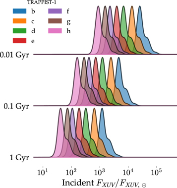
Figure 5. Updated  for each TRAPPIST-1 planet derived from samples drawn from the posterior distribution and simulated using VPLanet when the system was 0.01, 0.1, and 1 Gyr old. The latter age corresponds to the approximate age at which TRAPPIST-1 entered the main sequence. The TRAPPIST-1 planetary system has likely endured a long-lasting, extreme XUV environment.
Download figure:
Standard image High-resolution imageWe infer that TRAPPIST-1b likely received extreme  during the early pre-main-sequence before decaying to the present-day
  , consistent with estimates from Wheatley et al. (2017). The extended upper tail of the FXUV distributions corresponds to the large fsat values permitted by the posterior distributions. The likely habitable-zone planets, e, f, and g, similarly experienced severe XUV fluxes ranging in
  throughout the pre-main-sequence. Even today, e, f, and g receive
  , far in excess of the modern Earth, due to TRAPPIST-1's large present LXUV, its extended saturated phase, and the close proximity of M dwarf habitable-zone planets to their host star. These significant high-energy fluxes likely drove an extended epoch of substantial atmospheric escape and water loss from the TRAPPIST-1 planets, potentially producing substantial abiotic O2 atmospheres (Luger & Barnes 2015; Bolmont et al. 2017; Bourrier et al. 2017a).
4. Discussion and Conclusions
Here we used MCMC to derive probabilistic constraints for TRAPPIST-1's stellar and LXUV evolution to characterize the evolving XUV environment of its planetary system. We inferred that TRAPPIST-1 likely maintained high LXUV/Lbol ≈ 10−3 throughout its lifetime, with a 40% chance that TRAPPIST-1 is still in the saturated regime today. Our results indicate that at least some ultracool dwarfs can sustain large LXUV in the saturated regime for gigayears, consistent with the activity lifetimes of late M dwarfs (West et al. 2008). We suggest that studies of volatile loss from planets orbiting ultracool dwarfs model the long-term LXUV evolution of the host star, or at least assume saturation timescales of tsat ≳ 4 Gyr. Our choice of prior distributions strongly affects our results as our inference hinges on only two measured properties of TRAPPIST-1, LXUV and Lbol. To mitigate this effect, we consulted previous studies and empirical observations of the activity evolution of late M dwarfs to construct realistic prior distributions.
The TRAPPIST-1 planets likely experienced significant XUV fluxes during the pre-main-sequence, potentially driving extreme atmospheric erosion and water loss (Bolmont et al. 2017; Bourrier et al. 2017a). The high-energy fluxes incident on the innermost planets throughout this phase were probably large enough for atmospheric mass loss to be recombination-limited (FUV ≳ 104 g s−1 cm−2) and scale as  (Murray-Clay et al. 2009), as opposed to the oft-assumed energy-limited escape (
 , Watson et al. 1981; Lammer et al. 2003), potentially inhibiting volatile loss. If the TRAPPIST-1 planets did lose significant amounts of water as our estimates suggest, they must have formed with a large initial volatile inventory to account for their observed low densities (Grimm et al. 2018).
We demonstrated that the open source Python machine learning package approxposterior (Fleming & VanderPlas 2018) can efficiently compute an accurate approximation to the posterior distribution using an adaptive-learning GP-based method, requiring 1330 times fewer VPLanet simulations and a factor of 980 times less core hours than traditional MCMC approaches. The posterior distributions derived by approxposterior reproduced the nontrivial parameter correlations and best-fit values uncovered by our fiducial MCMC analysis. We find that approxposterior recovers the best-fit values and 1σ uncertainties of our model parameters with an average error of 0.61% and 5.5%, respectively, relative to our constraints derived using emcee. If future observations of TRAPPIST-1 refine its fundamental parameters, and possibly LXUV/Lbol, approxposterior can be used to rapidly and accurately replicate our analysis to update our constraints.
Finally, we note that our methodology constrains parameters that describe the long-term XUV evolution of TRAPPIST-1, conditioned on measurements. In principle, this approach can be extended to obtain evolutionary histories of planetary systems in general. For example, in Figures 4 and 5, we examined the long-term evolution of TRAPPIST-1 and the evolving XUV fluxes received by its planetary system, respectively, with samples drawn from the posterior distribution. Future research can combine those results with additional physical effects, for example, water loss or tidal dissipation, to build a probabilistic model for the long-term evolution of the planetary system, given our model for the underlying physics, to characterize its present state. In other words, we could infer the evolutionary history of a planet or planetary system given suitable observational constraints. While simulating additional physical effects will inevitably increase the computational expense, we have demonstrated that approxposterior can enable such efforts and provide insight into the histories of stars and their planets.
We thank the anonymous referee for their careful reading of our manuscript and insightful comments. This work was facilitated through the use of advanced computational, storage, and networking infrastructure provided by the Hyak supercomputer system and funded by the Student Technology Fund at the University of Washington. D.P.F. was supported by NASA Headquarters under the NASA Earth and Space Science Fellowship Program, grant 80NSSC17K0482. This work was supported by the NASA Astrobiology Program grant No. 80NSSC18K0829 and benefited from participation in the NASA Nexus for Exoplanet Systems Science research coordination network.
Software: approxposterior: Fleming & VanderPlas (2018), corner: Foreman-Mackey (2016), emcee: Foreman-Mackey et al. (2013), george: Ambikasaran et al. (2015), VPLanet: Barnes et al. (2020).
Appendix
approxposterior is an implementation of the "Bayesian Active Posterior Estimation" (BAPE) algorithm developed by Kandasamy et al. (2017), but with several modifications to afford the user more control over the inference. Below, we qualitatively describe this algorithm, define parameters, and suggest typical values. We then discuss approxposterior's convergence scheme.
Appendix A: approxposterior Algorithm and Convergence
Qualitatively, the approxposterior algorithm is as follows. First, assume a forward model with d input parameters that is designed to reproduce some set of observations. In our case, d, the dimensionality of parameter space, is five. The model parameters have an input domain, D, that is defined by the user. The parameters are further described by a prior probability distribution based on the user's prior belief for how the model parameters are distributed. Next, the user generates a training set, T, consisting of m0 forward-model simulations distributed across the parameter space. The user chooses how the m0 samples are distributed throughout parameter space according to their preferred experimental design. approxposterior then trains a GP on T to construct a nonparametric model (sometimes called a "surrogate model") that represents the outcomes of the forward model over the parameter space. Crucially, GPs also generate an uncertainty for the surrogate model at every point in parameter space.
approxposterior then identifies m more locations in parameter space to apply the forward model and add to T. The new locations are selected by determining the regions that the GP has identified as having both a high lnprobability, that is, a high posterior density, and a high predictive uncertainty. This selection is accomplished by maximizing a utility function (u, described below) that quantifies where the GP predicts a high posterior density and high uncertainty in parameter space, focusing resources on parameter combinations that are likely to be consistent with the observations. approxposterior retrains the GP with the augmented T. The GP is then passed to an MCMC algorithm, emcee, that samples the parameter space to obtain the approximate posterior distributions of the model parameters.
At the end of each iteration, approxposterior checks if a convergence condition (described in Appendix A.2) has been met. If the algorithm has not yet converged, approxposterior selects an additional m new points to add to T, retrains the GP, and again estimates the posterior distribution. This process repeats until convergence or until approxposterior has run the maximum number of iterations, nmax, set by the user. In Algorithm 1, we list the aforementioned steps that comprise this algorithm.
Algorithm 1. approxposterior Approximate Inference Pseudo Code
Download table as:
ASCIITypeset image
Assume an input domain D, GP prior on f(x)
Generate a training set, T, consisting of m0 pairs of

for

for

Find x+ = argmax

Compute

Append
 to T
to T
Retrain GP, optimize GP hyperparameters given augmented T
end
Use MCMC to obtain approximate posterior distribution with GP surrogate for

if
 break
break
end
end
where  +
+  , that is, the lnprobability function used for MCMC sampling with emcee, and x+ is the point in parameter space selected by maximizing u. For our application, evaluating
  requires running a VPLanet simulation to compute
  (see Section 2.4).
By placing a GP prior with a squared exponential kernel on  , we assume that the function is smooth and continuous, both reasonable assumptions for modeling the posterior density. For inference problems that are likely to violate these assumptions, other kernels, such as the Ornstein–Uhlenbeck kernel, may be more appropriate (we refer the reader to Rasmussen & Williams 2006 for detailed descriptions of common GP kernels and their mathematical properties). approxposterior uses george (Ambikasaran et al. 2015) for all GP calculations, and hence users can apply any kernels implemented in that software package.
approxposterior has several free parameters that can be set by the user: m0, the size of the initial training set (50 in our case);  , the maximum number of iterations (15); m, the number of new points to select each iteration where the forward model will be evaluated (50 per iteration); and
  , the convergence threshold (0.1). Typically, we find that
  ,
,  , and
, and  work well in practice, although performance may vary depending on the use case. For a complete list of approxposterior parameters, we refer the reader to the online documentation.9
Note that approxposterior does not linearly transform the parameter space to the unit hypercube as did Kandasamy et al. (2017). Moreover, approxposterior does not fix the covariance scale lengths, instead opting to estimate all GP kernel hyperparameters by maximizing the marginal likelihood of the GP, given its training set, at a user-specified cadence. In Algorithm 1, we optimize the GP hyperparameters each time a new point is added to the training set, but in practice we found this is unnecessary, especially at later iterations when the GP has developed a reasonable approximation of the posterior. The authors prefer to optimize the GP hyperparameters twice per iteration, once after half of the m new points have been selected, and again after all m points have been selected.
A.1. Augmenting the Training Set
Each iteration, approxposterior selects m new points to add to the GP's training set by maximizing the utility function, u. To motivate the choice of u, consider the following argument based on Kandasamy et al. (2017): approxposterior assumes that the forward model the GP learns on, here VPLanet via  , is computationally expensive to run, and hence approxposterior seeks to minimize the number of forward-model evaluations required to build its training set. For inference problems, it is natural to select high-lnprobability regions in parameter space to augment the GP training set as this is where the posterior density is large. Furthermore, selecting regions in parameter space where the GP's predictive uncertainty is already small offers little value, compared to regions where its predictions are more uncertain, as additional points in low-uncertainty regions are unlikely to alter the GP's predictions.
With these considerations in mind, Kandasamy et al. (2017) leverage the analytic properties of GPs to derive the "exponentiated variance" utility function, given by their Equation (5):

where  and
and  are the mean and variance of the GP's predictive conditional distribution evaluated at
  , respectively, for the tth approxposterior iteration. To select each point, we maximize Equation (5) using the Nelder–Mead method (Nelder & Mead 1965). Note that this optimization is rather cheap because it only requires evaluating the GP's predictive conditional distribution, so this task is not a significant computational bottleneck. We restart this optimization five times to reduce the influence of local extrema. Note that in practice, we optimize the natural logarithm of the utility function to ensure numerical stability.
As demonstrated in Kandasamy et al. (2017), Equation (5) identifies high-likelihood points where the GP's predictions are uncertain, significantly reducing the cost of training an accurate GP surrogate model. We highlight this behavior for our own application in Figure 6 by displaying the approximate posterior distribution derived by approxposterior from Figure 2 overplotted with the initial training set in orange and the points selected by sequentially maximizing Equation (5) in blue. Given the small initial training set, approxposterior successfully selects high-posterior-density points in parameter space to augment the GP's training set. Some points are selected in low-likelihood regions early on, typically near the edges of parameter space where the GP's uncertainty was initially large.
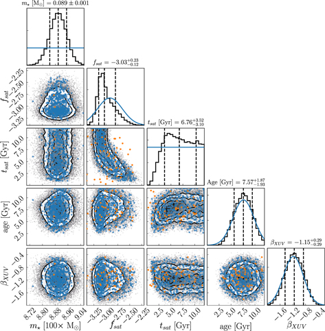
Figure 6. Same as Figure 2, but overplotted with the training set for approxposterior's GP. The orange points display the initial training points, whereas the blue points display the points iteratively selected by maximizing the Kandasamy et al. (2017) utility function, Equation (5). By design, approxposterior selected points to expand its training set in regions of high posterior density, improving its GP's predictive accuracy in the most relevant regions of parameter space while seldom wasting computational resources in the low-likelihood regions.
Download figure:
Standard image High-resolution imageA.2. Convergence
We assess the convergence of the approxposterior algorithm by comparing the means of the approximate marginal posterior distributions over successive iterations. We consider an approxposterior run "converged" if the differences between the marginal posterior means, relative to the widths of the marginal posteriors, are less than a tolerance parameter, , for kmax consecutive iterations. Effectively, this criterion checks if the expected value of each model parameter over the posterior distribution varies by  standard deviations from the previous iteration's expected values. That is, we require the approxposterior convergence diagnostic
  for all j, where

and μt,j and σt,j are the mean and standard deviation of the approximate marginal posterior distribution for the tth iteration and the jth parameter. This quantity is analogous to the "z-score" commonly used in many statistical tests. Following Wang & Li (2018), we require this condition to be satisfied for kmax consecutive iterations to ensure approxposterior is producing a consistent result. With this scheme, approxposterior tolerates deviations from the previous estimate that are less than, or at least consistent with, the previous values, given the inherent uncertainty implied by the width of the posterior distribution. For our application, we adopted conservative choices of = 0.1 and kmax = 5. For each approxposterior iteration, we also visually inspected the estimated posterior distribution to ensure convergence.
In Figure 7, we display the convergence diagnostic quantity, zt, as a function of iteration for each model parameter for the approxposterior run presented in the main text. approxposterior quickly finds a consistent result as zt decreases below our convergence threshold within the first few iterations. For each parameter, zt continues to decrease until iteration 3 before stabilizing. The evolution of zt is not monotonic, however, owing to the stochastic nature of GPs, our hyperparameter optimization scheme, and MCMC sampling that can cause these values to occasionally be slightly worse than previous iterations. Requiring convergence over kmax consecutive iterations mitigates the impact of this stochasticity.

Figure 7. The approxposterior convergence diagnostic, zt, as a function of iteration for the run presented in the main text. Note that in approxposterior, the initial iteration is iteration 0. The black dashed line indicates our adopted convergence threshold of = 0.1. approxposterior quickly converges to a consistent and accurate result.
Download figure:
Standard image High-resolution image
Footnotes
- 6
VPLanet is publicly available at https://github.com/VirtualPlanetaryLaboratory/vplanet.
- 7
- 8
approxposterior is publicly available at https://github.com/dflemin3/approxposterior.
- 9