


Abstract
We study the  luminosity line ratio in a sample of nearby (z < 0.05) galaxies: 25 star-forming galaxies (SFGs) from the xCOLD GASS survey, 36 hard X-ray-selected active galactic nucleus (AGN) host galaxies from the BAT AGN Spectroscopic Survey, and 37 infrared-luminous galaxies from the SCUBA Local Universe Galaxy Survey. We find a trend for r31 to increase with star formation efficiency (SFE). We model r31 using the UCL-PDR code and find that the gas density is the main parameter responsible for the variation of r31, while the interstellar radiation field and cosmic-ray ionization rate play only a minor role. We interpret these results to indicate a relation between SFE and gas density. We do not find a difference in the r31 value of SFGs and AGN host galaxies, when the galaxies are matched in SSFR (〈r31〉 = 0.52 ± 0.04 for SFGs and 〈r31〉 = 0.53 ± 0.06 for AGN hosts). According to the results of the UCL-PDR models, the X-rays can contribute to the enhancement of the CO line ratio, but only for strong X-ray fluxes and for high gas density (nH > 104 cm−3). We find a mild tightening of the Kennicutt–Schmidt relation when we use the molecular gas mass surface density traced by CO(3–2) (Pearson correlation coefficient R = 0.83), instead of the molecular gas mass surface density traced by CO(1–0) (R = 0.78), but the increase in correlation is not statistically significant (p-value = 0.06). This suggests that the CO(3–2) line can be reliably used to study the relation between SFR and molecular gas for normal SFGs at high redshift and to compare it with studies of low-redshift galaxies, as is common practice.
Export citation and abstract BibTeX RIS
1. Introduction
Star formation in galaxies is closely related to their gas content. This has been found in the correlation between the star formation rate (SFR) surface density and gas mass surface density (Kennicutt–Schmidt (KS) relation; Kennicutt 1998). The relation between SFR and molecular gas content is stronger than with the total gas content (Bigiel et al. 2008; Leroy et al. 2008; Saintonge et al. 2017). However, there is some scatter in this relation: the SFR surface density can vary by an order of magnitude for the same molecular gas mass surface density, measured from the CO(1–0) luminosity (Saintonge et al. 2012). A possible explanation is that CO(1–0) is a good tracer of the total molecular gas in massive galaxies, but it does not accurately trace the amount of gas located in the dense molecular cores where the formation of stars takes place (e.g., Solomon et al. 1992; Kohno et al. 2002; Shibatsuka et al. 2003). Because stars form in dense molecular clouds, it is reasonable to expect the SFR to correlate better with the amount of dense molecular gas than with the total (dense and diffuse) molecular gas. Commonly used tracers of dense gas are HCN, HCO+, or CS (e.g., Gao & Solomon 2004a, 2004b; Wu et al. 2010; Zhang et al. 2014; Tan et al. 2018).
Observations have shown that the HCN(1–0)/CO(1–0) ratio is enhanced in galaxies with high star formation efficiency (SFE = SFR/ ), like luminous infrared galaxies (LIRGs; Gao & Solomon 2004a; Gracia-Carpio et al. 2008; García-Burillo et al. 2012). However, the HCN(1–0) line flux is usually fainter than CO by more than an order of magnitude, making surveys of large samples of normal star-forming galaxies (SFGs) very time consuming. Another option is to use higher CO transitions to trace the mass of dense molecular gas. The ideal transition is CO(3–2): it does not trace low-density gas (critical density ncrit = 3.6 × 104 cm−3, calculated under the optically thin assumption; Carilli & Walter 2013) like the CO(1–0) and CO(2–1) transitions, and at the same time it does not require high temperatures to populate it (the minimum gas temperature needed for significant excitation is Tmin = 33 K; Mauersberger et al. 1999; Yao et al. 2003; Wilson et al. 2009). If the gas density is the key quantity regulating the relation between molecular gas mass and SFR, then we expect to see a correlation between the SFE and the r31
 luminosity line ratio, which can be interpreted as an indicator of the gas density.
The r31 value has been measured in samples of LIRGs (Leech et al. 2010; Papadopoulos et al. 2012), in the central regions of nearby galaxies (Mauersberger et al. 1999; Mao et al. 2010), in submillimeter galaxies (SMGs; Harris et al. 2010), and in nearby galaxies (Wilson et al. 2012). Yao et al. (2003) and Leech et al. (2010) found a trend where r31 increases with increasing SFE in samples of infrared-luminous galaxies and LIRGs. This trend has also been found in spatially resolved observations of M83, NGC 3627, and NGC 5055 (Muraoka et al. 2007; Morokuma-Matsui & Muraoka 2017). Sharon et al. (2016) found a similar trend in a sample of submillimeter galaxies and AGN hosts at redshifts z = 2–3. Most studies of the r31 line ratio focused on extreme objects, like LIRGs, or are limited to small samples. In this work, we collect CO observations for a homogeneous sample of main-sequence galaxies to investigate the r31 line ratio in more "normal" SFGs.
We also analyze a sample of galaxies hosting active galactic nuclei (AGN) to investigate if AGN have an effect on the r31 line ratio of their host galaxy. Several studies of the CO spectral line energy distribution (SLED) of AGN focused on the high-J rotational transition levels. For instance, Lu et al. (2017) studied the CO SLED in the GOALS sample (The Great Observatories All-Sky LIRG Survey; Armus et al. 2009) and found that the presence of an AGN influences only the very high J levels (J > 10). Mashian et al. (2015) found that the CO SLED is not the same in all AGN and that the shape of the CO SLED of a galaxy is more related to the content of warm and dense molecular gas than to the excitation mechanism. Rosenberg et al. (2015) analyzed the CO ladder of 29 objects from the Herschel Comprehensive ULIRG Emission Survey (HerCULES). They find that in objects with a large AGN contribution, the CO ladder peaks at higher J levels, which means that in these objects, the CO excitation is influenced by harder radiation sources (X-rays or cosmic rays). These studies focus mostly on the high J levels (J > 4). Rosario et al. (2018) studied the molecular gas properties, traced by CO(2–1), of a sample of 20 nearby (z < 0.01) hard X-ray-selected AGN hosts from the LLAMA survey and compared it with a control sample of SFGs. They found similar molecular gas fraction and SFE in the central region of AGN and in the control galaxies. Sharon et al. (2016) also compared the r31 values of 15 SMGs and 13 AGN host galaxies at redshifts z = 2–3 and did not find a significant difference.
In this paper, we study the r31 luminosity line ratio in a sample of nearby (z < 0.05) SFGs and AGN. In Sections 2 and 3, we describe the sample and the CO observations. In Section 4, we present the r31 values and analyze the correlation with SFR, SSFR, and SFE. We also compare the r31 values for AGN and SFGs. In Section 5, we use the modeling of the line ratio using a PDR (photodissociation region) code to test which parameters regulate the CO line ratios. Finally, in Section 6, we compare the KS relation with molecular gas masses derived using the CO(1–0) and CO(3–2) line emission.
Throughout this work, we assume a cosmological model with Ωλ = 0.7, ΩM = 0.3 , and H0 = 70 km s−1 Mpc−1.
2. Sample
2.1. Star-forming Galaxies: xCOLD GASS
The xCOLD GASS survey (Saintonge et al. 2011a, 2017) was designed to observe the CO(1–0) emission for ∼500 galaxies in order to establish the first unbiased scaling relations between the cold gas (atomic and molecular) contents of galaxies and their stellar, structural, and chemical properties. A sample of 25 galaxies from xCOLD GASS also has JCMT observations of the CO(3–2) emission line. The sample was selected based on the following criteria:
- 1.Good detection of the CO(1–0) line (signal-to-noise of the line >3).
- 2.CO(3–2) luminosity high enough to require less than two hours of integration time with the JCMT in band 3 (opacity
 ). Assuming r31 = 0.5, this requirement corresponds to CO(1–0) luminosities K km s−1 pc2.
 - 3.The targets were selected to span a broad range of specific star formation rates (, ) and SFEs (/, ).


The galaxies in the sample are in the redshift interval 0.026 < z < 0.049. They have stellar masses in the range 10 < log M*/M⊙ < 11 and SFRs in the range ![$-0.05\,\lt \mathrm{logSFR}/[{M}_{\odot }{\mathrm{yr}}^{-1}]\lt 1.54$](https://content.cld.iop.org/journals/0004-637X/889/2/103/revision1/apjab6221ieqn12.gif) .
.
All the galaxy properties are taken from the xCOLD GASS catalog (Saintonge et al. 2017). In particular, SFRs are calculated by combining the IR- and UV-based SFR components obtained from Wide-field Infrared Survey Explorer (WISE) and GALEX photometry, as described in Janowiecki et al. (2017). Stellar masses come from the Sloan Digital Sky Survey (SDSS) DR7 MPA/JHU catalog.11 The 25 galaxies with CO(3–2) observations are not classified as AGN by the optical emission-line diagnostics BPT diagram (Baldwin et al. 1981; Kewley et al. 2001; Kauffmann et al. 2003). Four objects are classified as composite, one as a LINER, and the remaining galaxies are classified as star-forming. The properties of the sample are summarized in Table 1.
Table 1. Properties of the xCOLD GASS Sample
| Index | R.A. | Decl. | z | D25 | log M* | log SFR | 
|
log M(H2) |
|---|---|---|---|---|---|---|---|---|
| (deg) | (deg) | (arcsec) | (log  ) ) |
(log  yr−1) yr−1) |

|
(log  ) ) |
||
| 522 | 171.07767 | 0.64373 | 0.02637 | 51.7 | 10.08 | 0.40 | 4.35 | 9.13 |
| 1115 | 214.56213 | 0.89111 | 0.02595 | 69.3 | 10.11 | 0.76 | 4.35 | 9.61 |
| 1137 | 215.81121 | 0.97835 | 0.04007 | 38.8 | 10.28 | 0.56 | 4.35 | 9.42 |
| 1221 | 218.85558 | 0.33433 | 0.03455 | 23.4 | 10.20 | 0.84 | 4.35 | 9.73 |
| 3819 | 25.42996 | 13.67579 | 0.04531 | 27.7 | 10.67 | 1.03 | 4.35 | 9.98 |
| 3962 | 30.99646 | 14.31038 | 0.04274 | 46.3 | 10.90 | 0.80 | 4.35 | 10.06 |
| 4045 | 32.88983 | 13.91716 | 0.02651 | 43.5 | 10.47 | 0.66 | 4.35 | 9.71 |
| 7493 | 216.83387 | 2.83838 | 0.02644 | 46.1 | 10.56 | 0.41 | 4.35 | 9.64 |
| 9551 | 216.88492 | 4.82163 | 0.02688 | 60.3 | 10.91 | 0.28 | 4.35 | 9.97 |
| 11112 | 345.66796 | 13.32907 | 0.02765 | 51.6 | 10.81 | 0.46 | 4.35 | 9.85 |
| 11223 | 346.56850 | 13.98231 | 0.03554 | 33.6 | 10.64 | 0.67 | 4.35 | 9.94 |
| 11408 | 350.61417 | 13.81586 | 0.026 | 45.4 | 10.05 | 0.08 | 4.35 | 9.12 |
| 14712 | 139.74192 | 5.88840 | 0.03827 | 35.5 | 10.55 | 0.63 | 4.35 | 9.82 |
| 15155 | 160.22996 | 5.99141 | 0.02773 | 79.6 | 10.19 | 0.57 | 4.35 | 9.88 |
| 22436 | 139.97725 | 32.93328 | 0.04916 | 58.8 | 10.42 | 1.54 | 1.00 | 9.75 |
| 23194 | 158.38929 | 11.87138 | 0.03404 | 41.0 | 10.59 | 0.70 | 1.00 | 9.22 |
| 23245 | 160.91283 | 12.06066 | 0.02623 | 42.9 | 10.11 | −0.05 | 4.35 | 8.76 |
| 24973 | 218.82654 | 35.11868 | 0.0285 | 47.5 | 10.61 | 1.09 | 1.00 | 9.33 |
| 25327 | 203.10100 | 11.10636 | 0.03144 | 41.6 | 10.03 | 1.40 | 1.00 | 9.72 |
| 25763 | 135.79688 | 10.15197 | 0.02962 | 54.0 | 10.11 | 0.22 | 4.35 | 9.39 |
| 26221 | 154.15996 | 12.57738 | 0.03166 | 75.5 | 10.98 | 0.57 | 4.35 | 10.07 |
| 28365 | 235.34412 | 28.22975 | 0.03209 | 56.1 | 10.36 | 0.60 | 4.35 | 9.65 |
| 40439 | 196.06267 | 9.22346 | 0.03501 | 70.8 | 10.95 | 0.73 | 4.35 | 9.89 |
| 42013 | 229.01862 | 6.84763 | 0.03681 | 39.7 | 10.77 | 0.70 | 4.35 | 9.96 |
| 48369 | 167.80421 | 28.71190 | 0.02931 | 20.2 | 10.32 | 0.67 | 1.00 | 9.42 |
Download table as: ASCIITypeset image
2.2. Active Galactic Nuclei: BASS
We include in our study a sample of AGN selected in the hard X-ray from the Swift/BAT 70 Month survey (Baumgartner et al. 2013). We have CO(3–2) observations of 46 BAT AGN at redshift <0.04. In our analysis, we focus on sources for which we also have observations of the CO(2–1) transition. Additionally, we discard from our sample three AGN for which Herschel FIR observations are not available and thus we cannot infer their SFR. Thus, the final BASS sample that we use in our analysis consists of 36 objects. These sources are part of the BAT AGN Spectroscopic Survey (BASS12 ), for which ancillary information from optical and X-ray spectroscopic analysis is available (Koss et al. 2017; Ricci et al. 2017). The AGN are in the redshift range 0.002 < z < 0.040.
The SFR is inferred from the total (8–1000 μm) infrared (IR) luminosity due to star formation given in Shimizu et al. (2017), which was measured by decomposing the IR spectral energy distribution (SED) in the AGN and host galaxy component. We use the following conversion from total IR luminosity (3–1100 μm range) to SFR, calculated assuming a Kroupa IMF (Hao et al. 2011; Murphy et al. 2011; Kennicutt & Evans 2012):

where the SFR is in units of M⊙ yr−1 and LIR is the total IR luminosity in erg s−1.
We use stellar masses measured for BAT AGN host galaxies from N. Secrest et al. (2020, in preparation). They are derived by spectrally deconvolving the AGN emission from stellar emission via SED decomposition, combining near-IR data from the Two Micron All Sky Survey (2MASS), which is more sensitive to stellar emission, with mid-IR data from the AllWISE catalog (Wright et al. 2010), which is more sensitive to AGN emission. The galaxies in the sample have stellar masses in the range  and SFR in the range
 ![$-0.83\lt \mathrm{logSFR}/[{M}_{\odot }{\mathrm{yr}}^{-1}]\lt 1.75$](https://content.cld.iop.org/journals/0004-637X/889/2/103/revision1/apjab6221ieqn19.gif) . Table 2 lists the properties of this sample.
. Table 2 lists the properties of this sample.
Table 2. Properties of the BASS Sample
| BAT | Name | R.A. | Decl. | z | Rk20 | log M* | log SFR | 
|
log M(H2) |
|---|---|---|---|---|---|---|---|---|---|
| Index | (deg) | (deg) | (arcsec) | (log  ) ) |
(log  yr−1) yr−1) |

|
(log  ) ) |
||
| 144 | NGC 1068 | 40.66960 | −0.01330 | 0.00303 | 95.0 | 10.54 | ⋯ | 4.35 | 9.79 |
| 173 | NGC 1275 | 49.95070 | 41.51170 | 0.01658 | 62.9 | 11.13 | ⋯ | 4.35 | ⋯ |
| 228 | Mrk 618 | 69.09300 | −10.37600 | 0.03464 | 18.1 | 10.62 | 1.19 | 4.35 | 10.19 |
| 308 | NGC 2110 | 88.04740 | −7.45620 | 0.00739 | 54.9 | 10.56 | 0.15 | 4.35 | 8.62 |
| 310 | MCG +08-11-011 | 88.72340 | 46.43930 | 0.02019 | 54.8 | 10.72 | −0.43 | 4.35 | 9.84 |
| 316 | IRAS 05589 + 2828 | 90.54365 | 28.47205 | 0.03309 | 0.0 | 10.57 | 0.35 | 4.35 | 9.75 |
| 337 | VIIZW 073 | 98.19654 | 63.67367 | 0.04042 | 34.3 | 10.46 | 1.13 | 4.35 | 9.98 |
| 382 | Mrk 79 | 115.63670 | 49.80970 | 0.02213 | 30.9 | 10.49 | 0.46 | 4.35 | ⋯ |
| 399 | 2MASX J07595347 + 2323241 | 119.97280 | 23.39010 | 0.02894 | 21.1 | 10.72 | ⋯ | 4.35 | 10.32 |
| 400 | IC 0486 | 120.08740 | 26.61350 | 0.02656 | 19.9 | 10.57 | 0.49 | 4.35 | 9.75 |
| 404 | Mrk 1210 | 121.02440 | 5.11380 | 0.01354 | 15.2 | 9.93 | −0.18 | 4.35 | ⋯ |
| 405 | MCG +02-21-013 | 121.19330 | 10.77670 | 0.03486 | 19.6 | 10.76 | 0.33 | 4.35 | 10.28 |
| 439 | Mrk 18 | 135.49300 | 60.15200 | 0.01101 | 18.0 | 9.74 | 0.01 | 4.35 | 8.73 |
| 451 | IC 2461 | 139.99200 | 37.19100 | 0.00753 | 40.5 | 10.06 | −0.45 | 4.35 | 9.20 |
| 471 | NGC 2992 | 146.42520 | −14.32640 | 0.00757 | 50.9 | 10.22 | 0.34 | 4.35 | 9.30 |
| 480 | NGC 3081 | 149.87310 | −22.82630 | 0.00763 | 54.3 | 9.96 | −0.33 | 4.35 | 8.85 |
| 497 | NGC 3227 | 155.87740 | 19.86510 | 0.00329 | 92.6 | 10.06 | 0.35 | 4.35 | 9.74 |
| 517 | UGC 05881 | 161.67700 | 25.93130 | 0.02048 | 14.5 | 10.17 | 0.42 | 4.35 | 9.42 |
| 530 | NGC 3516 | 166.69790 | 72.56860 | 0.00871 | 40.8 | 10.65 | −0.28 | 4.35 | 8.73 |
| 532 | IC 2637 | 168.45700 | 9.58600 | 0.02915 | 18.1 | 10.60 | 1.04 | 4.35 | 10.10 |
| 548 | NGC 3718 | 173.14520 | 53.06790 | 0.00279 | 75.5 | 10.03 | −0.83 | 4.35 | 8.49 |
| 552 | Mrk 739E | 174.12200 | 21.59600 | 0.02945 | 20.4 | 10.60 | 0.89 | 4.35 | 9.98 |
| 560 | NGC 3786 | 174.92700 | 31.90900 | 0.00897 | 49.0 | 10.32 | −0.06 | 4.35 | 9.52 |
| 585 | NGC 4051 | 180.79010 | 44.53130 | 0.00203 | 102.6 | 9.82 | 0.17 | 4.35 | 9.80 |
| 588 | UGC 07064 | 181.18060 | 31.17730 | 0.02508 | 21.9 | 10.60 | 0.76 | 4.35 | 10.10 |
| 590 | NGC 4102 | 181.59630 | 52.71090 | 0.00185 | 68.6 | 10.18 | 0.54 | 4.35 | 9.57 |
| 599 | NGC 4180 | 183.26200 | 7.03800 | 0.00700 | 40.0 | 9.96 | 0.17 | 4.35 | ⋯ |
| 608 | Mrk 766 | 184.61050 | 29.81290 | 0.01292 | 25.6 | 10.11 | 0.35 | 4.35 | 9.26 |
| 609 | M106 | 184.73960 | 47.30400 | 0.00168 | 263.9 | 10.22 | −0.10 | 4.35 | 9.29 |
| 615 | NGC 4388 | 186.44480 | 12.66210 | 0.00834 | 92.9 | 10.08 | −0.09 | 4.35 | 7.91 |
| 631 | NGC 4593 | 189.91430 | −5.34430 | 0.00835 | 80.6 | 10.46 | ⋯ | 4.35 | 9.24 |
| 669 | NGC 5100NED02 | 200.24830 | 8.97830 | 0.03259 | 21.9 | 10.71 | 1.19 | 4.35 | ⋯ |
| 670 | MCG -03-34-064 | 200.60190 | −16.72860 | 0.01682 | 25.3 | 10.47 | 0.68 | 4.35 | 9.34 |
| 688 | NGC 5290 | 206.32990 | 41.71260 | 0.00854 | 89.0 | 10.39 | −0.03 | 4.35 | 9.86 |
| 703 | Mrk 463 | 209.01200 | 18.37210 | 0.05015 | 14.0 | 10.59 | ⋯ | 4.35 | ⋯ |
| 712 | NGC 5506 | 213.31190 | −3.20750 | 0.00609 | 74.6 | 9.92 | −0.26 | 4.35 | 8.84 |
| 723 | NGC 5610 | 216.09540 | 24.61440 | 0.01691 | 39.4 | 10.34 | 0.70 | 4.35 | 9.91 |
| 739 | NGC 5728 | 220.59970 | −17.25320 | 0.00990 | 80.4 | 10.31 | 0.19 | 4.35 | 9.34 |
| 766 | NGC 5899 | 228.76350 | 42.04990 | 0.00844 | 67.8 | 10.37 | 0.54 | 4.35 | 9.74 |
| 772 | MCG -01-40-001 | 233.33630 | −8.70050 | 0.02285 | 43.7 | 10.57 | 0.81 | 4.35 | 9.84 |
| 783 | NGC 5995 | 237.10400 | −13.75780 | 0.02442 | 24.3 | 10.87 | 1.04 | 4.35 | 10.18 |
| 841 | NGC 6240 | 253.24540 | 2.40090 | 0.02386 | 39.9 | 11.02 | 1.75 | 1.00 | 10.07 |
| 1042 | 2MASX J19373299–0613046 | 294.38800 | −6.21800 | 0.01036 | 19.8 | 9.97 | −0.17 | 4.35 | 9.29 |
| 1046 | NGC 6814 | 295.66940 | −10.32350 | 0.00576 | 71.7 | 10.32 | 0.14 | 4.35 | 9.16 |
| 1133 | Mrk 520 | 330.17242 | 10.55221 | 0.02753 | 14.4 | 10.33 | ⋯ | 4.35 | ⋯ |
| 1184 | NGC 7479 | 346.23610 | 12.32290 | 0.00705 | 87.9 | 10.41 | 0.57 | 4.35 | 9.86 |
Download table as: ASCIITypeset image
2.3. Infrared-luminous Galaxies: SLUGS
We also include in our analysis a sample of IR-luminous galaxies ( ) from the SCUBA Local Universe Galaxy Survey (SLUGS; Dunne et al. 2000). We include this sample in order to extend the parameter range to galaxies with higher SFRs. We chose this sample over other samples available in the literature because it has beam-matched observations and information about how to scale the total SFR to the SFR within the beam.
We select the 38 SLUGS galaxies with observations of both CO(3–2) and CO(1–0) available in Yao et al. (2003). These galaxies are in the redshift range 0.006 < z < 0.048. Stellar masses from the SDSS DR7 MPA/JHU catalog are available for only 22 galaxies of this sample and are in the range  .
.
We use the optical emission-line diagnostic (Baldwin et al. 1981; Kewley et al. 2001; Kauffmann et al. 2003) from SDSS DR12 to distinguish between AGN and SFGs. Of the 22 galaxies with stellar masses from SDSS, two are classified as Seyferts (IRAS 10173+0828 and Arp 220), seven as Composite, and 13 as SFGs. We include the galaxies classified as Composite in the SFG sample.
The total SFRs are derived from the total IR luminosities LIR using Equation (1). We measure LIR by integrating the SED, approximated by a modified blackbody (MBB), in the range 8–1000 μm. The parameters of the MBB model are given in Dunne et al. (2000). We calculate the uncertainties on LIR by propagating the uncertainties on the MBB parameters given in Dunne et al. (2000). The SFRs are in the range 0.18 < log SFR/[ yr−1] < 2.15. Yao et al. (2003) also provide the FIR luminosity and SFR corresponding to the 15'' central part of the galaxy (equivalent to the size of the CO beam), obtained by applying a scale factor to the total FIR luminosity. This factor is derived from the original 850 μm SCUBA-2 images. To calculate the SFE, we use the SFR in the 15'' central part of the galaxy, as it matches the beam size of the CO observations.
We note that for this sample the molecular gas mass  , and consequently also the SFE, represents only the value in the central 15'' region of the galaxy, as no correction has been applied to extrapolate from the beam area to the total
  .
.
2.4. Samples in the SFR–M* Plane
Figure 1 shows the distribution of the xCOLD GASS, BASS, and SLUGS samples in the SFR–M* plane. The position of the star formation main sequence (Saintonge et al. 2016) is shown by the dashed line, and the dotted lines show the 0.4 dex dispersion. The "full xCOLD GASS" sample is shown by the gray points for reference. The three samples cover a similar range in stellar masses. All galaxies from the xCOLD GASS sample are on the main sequence or above, while the IR-luminous galaxies from the SLUGs sample are mostly above the main sequence. The BASS sample spans a broad range of specific star formation rate (SSFR), with ∼8 AGN below the main sequence and the rest of the sample overlapping in the parameter space with the xCOLD GASS galaxies. The right panel of Figure 1 shows the SSFR versus the SFE. The three samples span a similar range of SSFRs (−11 < log SSFR/[yr−1] < −8.5). The galaxies of the xCOLD GASS sample have slightly higher SFEs than the BASS galaxies at the same SSFR, but there is a good overlap with the BASS sample. The IR-luminous galaxies from SLUGS have in general high SSFR and high SFE.

Figure 1. Left: distribution of the xCOLD GASS, BASS, and SLUGS samples in the SFR–M* plane. The position of the star formation main sequence (Saintonge et al. 2016) is shown by the dashed line; the 0.4 dex dispersion is shown by dotted lines. The full xCOLD GASS sample is shown by the gray points, while the subsample with CO(3–2) observations is shown in magenta. Right: SSFR vs. star SFE (SFE = SFR/ ). Galaxies from the BASS sample have in general lower SFE than the xCOLD GASS galaxies at the same SSFR. For the SLUGS sample, we plot only the galaxies with angular diameter D < 100'', as their SFE is measured within the beam, while the SSFR is the total value.
Download figure:
Standard image High-resolution image3. CO Data, Observations, and Data Reduction
3.1. xCOLD GASS
3.1.1. xCOLD GASS: CO(1–0) Data from the Literature
The CO(1–0) line luminosities  are taken from the xCOLD GASS catalog (Saintonge et al. 2017). The CO(1–0) line fluxes are observed with the IRAM 30 m telescope (beam size: 22''). The 25 galaxies from xCOLD GASS selected for the CO(3–2) observations all have signal-to-noise ratio (S/N) > 3 in CO(1–0). We refer to Saintonge et al. (2017) for information about the observations and data reduction.
3.1.2. xCOLD GASS: CO(3–2) Observations
The CO(3–2) observations are taken with the HARP instrument (Heterodyne Array Receiver Program, beam size: 14''; Buckle et al. 2009) on the James Clerk Maxwell Telescope (JCMT; observing program M14AU21, PI: A. Saintonge). These observations took place between January and June 2014. Each CO(3–2) spectrum was observed in a single HARP pointing in "hybrid" mode, which produces two spectra for every scan (in two spectral windows). The spectra were reduced using the Starlink software (Currie et al. 2014). First, the two spectra within each scan were combined, after correcting for any baseline difference, and then all scans were combined together. A linear fit to the continuum was used to remove the baseline and then the spectrum was binned to a resolution of 40 km s−1.
The HARP instrument has 4 × 4 receptors (pixels), each one with a half-power beam width of 14''. We extract the CO(3–2) spectrum only from the pixel that is centered on the galaxy. The technique used to measure the flux from the reduced spectrum is the same used for the main xCOLD GASS survey (Saintonge et al. 2017). We convert the antenna temperature to flux units by applying the point source sensitivity factor 30 Jy K−1 recommended for HARP.13 We measure the velocity-integrated line flux SCO in Jy km s−1 by adding the signal within a spectral window. We initially set the width of the spectral window (WCO) equal to the FWHM of the CO(1–0) given in the xCOLD GASS catalog. In case the CO(3–2) line is clearly wider, we extend WCO to cover the total line emission. We determine the center of the line based on the SDSS spectroscopic redshift. In two cases where the CO(3–2) is clearly shifted with respect to the position determined from the SDSS redshift, we use the redshift of the CO(1–0) line, which is shifted in the same direction as the CO(3–2) line, to center the CO(3–2) line. We measure the baseline rms noise of the line-free channels (σCO) per 40 km s−1 channel in the spectral regions around the CO line.
The beam-integrated CO(3–2) line luminosity in units of K km s−1 pc2 is defined following Solomon et al. (1997) as

where  is the velocity-integrated CO(3–2) line flux within the HARP beam in units of Jy km s−1, νobs is the observed frequency of the CO(3–2) line in GHz, and DL is the luminosity distance in Mpc. The error on the line flux is defined as
where σCO is the rms noise achieved around the CO(3–2) line in spectral channels with width Δwch = 40 km s−1 and WCO the width (in km s−1) of the spectral window where we integrate the CO(3–2) line flux.
We use a detection threshold of S/N > 3, defined as S/N  , which is the same adopted for the main xCOLD GASS catalog. In 7 of 25 galaxies, the CO(3–2) line is not detected and we use conservative upper limits equal to five times the error:
  . The 5σ upper limits correspond to a "false negative" fraction of 2%, which is the probability that a source with "true" flux higher than this upper limit is not detected. To calculate
  we use the FWHM of the CO(1–0) line as an approximation for the width of the CO(3–2) line (
 ). All of the CO(3–2) spectra from xCOLD GASS are shown in the Appendix (Figure 8) and the measured line properties in Table 3.
Table 3. CO(3–2) Measurements for the xCOLD GASS Sample
| Index |
 rms rms |
S/N
|
flag
|

|

|

|
r31 | Beam Corr. |
|---|---|---|---|---|---|---|---|---|
| (mK) | (Jy km s−1) | (log K km s−1 pc2) | (log K km s−1 pc2) | 14'' to 22'' | ||||
| (1) | (2) | (3) | (4) | (5) | (6) | (7) | (8) | (9) |
| 522 | 3.00 | 3.47 | 1 | 22.63 ± 3.67 | 7.90 ± 0.13 | 8.34 ± 0.07 | 0.54 ± 0.18 | 1.48 |
| 1115 | 2.73 | 6.62 | 1 | 50.81 ± 8.24 | 8.24 ± 0.07 | 8.75 ± 0.07 | 0.43 ± 0.09 | 1.41 |
| 1137 | 1.80 | −1.83 | 2 | −7.37 ± 3.58 | <8.10 | 8.72 ± 0.05 | <0.31 | 1.28 |
| 1221 | 2.22 | 12.03 | 1 | 76.36 ± 8.69 | 8.67 ± 0.04 | 9.04 ± 0.04 | 0.50 ± 0.07 | 1.18 |
| 3819 | 4.56 | 6.53 | 1 | 86.85 ± 9.42 | 8.96 ± 0.07 | 9.30 ± 0.04 | 0.52 ± 0.10 | 1.15 |
| 3962 | 6.52 | 1.33 | 2 | 29.70 ± 11.12 | <9.01 | 9.35 ± 0.04 | <0.55 | 1.19 |
| 4045 | 7.50 | 8.56 | 1 | 139.84 ± 13.38 | 8.70 ± 0.05 | 9.03 ± 0.04 | 0.53 ± 0.08 | 1.15 |
| 7493 | 2.24 | 9.32 | 1 | 87.24 ± 12.32 | 8.49 ± 0.05 | 8.93 ± 0.05 | 0.44 ± 0.07 | 1.23 |
| 9551 | 3.06 | 10.97 | 1 | 152.23 ± 22.25 | 8.75 ± 0.04 | 9.25 ± 0.04 | 0.40 ± 0.05 | 1.27 |
| 11112 | 2.07 | 0.04 | 2 | 0.38 ± 16.14 | <8.19 | 9.11 ± 0.05 | <0.16 | 1.36 |
| 11223 | 3.24 | 8.65 | 1 | 118.99 ± 12.47 | 8.88 ± 0.05 | 9.24 ± 0.04 | 0.51 ± 0.08 | 1.17 |
| 11408 | 3.99 | −0.09 | 2 | −0.79 ± 3.63 | <7.98 | 8.36 ± 0.06 | <0.60 | 1.44 |
| 14712 | 3.87 | −0.38 | 2 | −4.21 ± 8.72 | <8.53 | 9.12 ± 0.04 | <0.34 | 1.33 |
| 15155 | 1.14 | 16.03 | 1 | 76.42 ± 14.23 | 8.47 ± 0.03 | 9.07 ± 0.05 | 0.34 ± 0.05 | 1.35 |
| 22436 | 2.88 | 16.83 | 1 | 277.51 ± 16.61 | 9.54 ± 0.03 | 9.64 ± 0.05 | 0.97 ± 0.12 | 1.24 |
| 23194 | 4.32 | 12.70 | 1 | 209.96 ± 11.39 | 9.09 ± 0.03 | 9.15 ± 0.05 | 1.15 ± 0.15 | 1.30 |
| 23245 | 3.68 | 2.18 | 2 | 17.48 ± 2.17 | <7.79 | 8.05 ± 0.06 | <0.84 | 1.53 |
| 24973 | 8.11 | 12.31 | 1 | 218.30 ± 18.02 | 8.95 ± 0.04 | 9.22 ± 0.05 | 0.71 ± 0.09 | 1.32 |
| 25327 | 7.48 | 23.79 | 1 | 677.88 ± 43.03 | 9.53 ± 0.02 | 9.69 ± 0.04 | 0.79 ± 0.08 | 1.14 |
| 25763 | 5.56 | −0.15 | 2 | −1.77 ± 4.66 | <8.31 | 8.57 ± 0.07 | <0.75 | 1.36 |
| 26221 | 3.17 | 12.09 | 1 | 161.63 ± 17.63 | 8.91 ± 0.04 | 9.30 ± 0.05 | 0.54 ± 0.07 | 1.31 |
| 28365 | 3.22 | 4.65 | 1 | 33.01 ± 7.23 | 8.24 ± 0.09 | 8.89 ± 0.05 | 0.33 ± 0.08 | 1.49 |
| 40439 | 1.92 | 3.15 | 1 | 20.48 ± 7.69 | 8.11 ± 0.14 | 8.96 ± 0.08 | 0.25 ± 0.09 | 1.80 |
| 42013 | 3.81 | 6.81 | 1 | 100.05 ± 13.38 | 8.84 ± 0.06 | 9.27 ± 0.04 | 0.43 ± 0.08 | 1.16 |
| 48369 | 3.99 | 18.72 | 1 | 283.35 ± 26.96 | 9.09 ± 0.02 | 9.41 ± 0.04 | 0.52 ± 0.05 | 1.08 |
Note. (1) Index. (2) Standard deviation of the noise. (3) Integrated S/N of the CO(3–2) line. (4) Flag for the detection of the CO(3–2) line based on a peak S/N > 3. 1: Detected, 2: non-detected. (5) Velocity-integrated flux  within the 14'' JCMT HARP beam. (6) CO(3–2) luminosity within the 14'' JCMT HARP beam. (7) CO(1–0) luminosity within the 22'' IRAM beam. (8) Beam-corrected luminosity ratio
  . (9) Beam-correction factor for extrapolating the CO(3–2) flux from the 14'' JCMT HARP to the 22'' IRAM beam.
Download table as: ASCIITypeset image
3.2. BASS
Both the CO(2–1) and CO(3–2) lines have been observed at the JCMT: the CO(3–2) with HARP and the CO(2–1) with the RxA instrument (beam size: 20''). The HARP observations took place in weather bands 3–4 (corresponding to an opacity  ), while the RxA observations took place in weather band 5 (
 ). The observations and data reduction of the CO(2–1) line emission are explained in detail in M. Koss et al. (2020, in preparation).
The CO(3–2) observations were taken between 2011 February and 2012 November in programs M11AH42C (PI: E. Treister) and M12BH03E (PI: M. Koss). Additionally, we also include 13 spectra from archival observations. Each galaxy was initially observed for 30 minutes. For weak detections, additional observations were obtained up to no more than two hours. The individual scans for a single galaxy were first-order baseline-subtracted and then coadded. We extract the CO(3–2) spectrum only from the pixel centered on the galaxy. We measure the CO(3–2) and CO(2–1) line fluxes using the same method as for the xCOLD GASS sample, for consistency. We measure the  line flux in Jy km s−1 by adding the signal within a spectral range that covers the entire width of the line. In the Appendix, we show the CO(3–2) spectra from BASS, in which we highlight the spectral regions where we integrate the fluxes. All BASS objects have good detections (i.e., S/N > 3) of the CO(2–1) lines, while we have non-detections (i.e., S/N < 3) in the CO(3–2) line for 3 of 36 galaxies. For these galaxies, we use upper limits equal to five times the flux error:
  .
.
Our set of observations is not homogeneous because for the xCOLD GASS and SLUGS samples, we compare the CO(3–2) to the CO(1–0) line, but for the BASS sample, we have to estimate CO(1–0) from the CO(2–1) line. Therefore, we need to assume a value for the ratio  . The typical value observed for normal spiral galaxies is r21 = 0.8 (Leroy et al. 2009; Saintonge et al. 2017). Leroy et al. (2009) studied a sample of 10 nearby spiral galaxies and found r21 values between 0.48 and 1.06, with most values in the range 0.6–1.0. They found an average of 0.81. For the xCOLD GASS survey, Saintonge et al. (2017) found a mean value of r21 = 0.79 ± 0.03 using a sample of 28 galaxies.
Some of the AGN in our sample (12/36) have recently been observed with the IRAM 30 m telescope as part of a program to measure CO(1–0) line luminosity for 133 BAT AGN (PI: T. Shimizu). We compute the r21 line ratios for these 12 objects using the values from T. T. Shimizu et al. (2020, in preparation). Because the difference in beam size is very small (IRAM: 22'', JCMT RxA: 20''), we did not apply any beam corrections. The r21 line ratios for these 12 objects are in the range 0.4–2.1, with a median r21 = 0.72. We obtain a robust standard deviation by computing the median absolute deviation MAD = 0.17. The robust standard deviation, under the assumption of a normal distribution, is given by  (Hoaglin et al. 1983). For the 12 objects with CO(1–0) observations, we use the CO(1–0) luminosities from T. T. Shimizu et al. (2020, in preparation) to compute the r31 line ratio. For the remaining AGN, we use a constant r21 = 0.72, and we assume an uncertainty of 0.26 on this value. The CO line fluxes for this sample are shown in Table 4.
Table 4. CO(3–2) and CO(2–1) Measurements for the BASS Sample
| BAT | S/N | Flag |

|

|

|
r31 | Beam Corr. | Beam Corr. Tot |
|---|---|---|---|---|---|---|---|---|
| Index | CO(32) | CO(32) | (Jy km s−1) | (log K km s−1 pc2) | (log K km s−1 pc2) | 14'' to 20'' | 20'' to Total | |
| (1) | (2) | (3) | (4) | (5) | (6) | (7) | (8) | (9) |
| 144 | 87.30 | 1 | 2787.72 ± 251.40 | 8.08 ± 0.00 | 8.49 ± 0.00 | 0.61 ± 0.00 | 1.95* | 3.62* |
| 173 | 24.65 | 1 | 198.29 ± 21.54 | 8.44 ± 0.02 | ⋯ | ⋯ | 1.80* | 2.32* |
| 228 | 13.39 | 1 | 159.38 ± 40.79 | 8.99 ± 0.03 | 9.26 ± 0.04 | 0.48 ± 0.13 | 1.13 | 1.54 |
| 308 | 23.52 | 1 | 132.00 ± 11.37 | 7.65 ± 0.02 | 7.65 ± 0.02 | 1.01 ± 0.26 | 1.25 | 1.73 |
| 310 | 12.13 | 1 | 72.27 ± 10.06 | 8.17 ± 0.04 | 8.32 ± 0.11 | 0.52 ± 0.07 | 1.31 | 4.33 |
| 316 | 3.83 | 1 | 62.35 ± 10.48 | 8.54 ± 0.11 | 8.76 ± 0.00 | 0.54 ± 0.20 | 1.14 | 1.80 |
| 337 | −0.97 | 2 | −25.80 ± 40.08 | <9.04 | 8.86 ± 0.10 | <0.92 | 1.14 | 1.63 |
| 382 | 7.05 | 1 | 51.22 ± 9.23 | 8.10 ± 0.06 | ⋯ | ⋯ | 1.31 | 2.50 |
| 399 | 7.70 | 1 | 153.57 ± 18.33 | 8.81 ± 0.06 | 9.20 ± 0.04 | 0.25 ± 0.03 | 1.16* | 1.61* |
| 400 | 2.09 | 2 | 31.28 ± 21.74 | <8.43 | 9.09 ± 0.08 | <0.53 | 1.17 | 2.21 |
| 404 | 8.81 | 1 | 49.19 ± 12.64 | 7.66 ± 0.05 | ⋯ | ⋯ | 1.09 | 1.92 |
| 405 | 5.08 | 1 | 72.40 ± 19.39 | 8.65 ± 0.09 | 8.81 ± 0.12 | 0.22 ± 0.04 | 1.14 | 1.91 |
| 439 | 10.14 | 1 | 88.24 ± 13.24 | 7.73 ± 0.04 | 7.80 ± 0.10 | 0.69 ± 0.10 | 1.08 | 1.46 |
| 451 | 6.49 | 1 | 47.50 ± 10.23 | 7.58 ± 0.07 | 8.09 ± 0.06 | 0.33 ± 0.11 | 1.33 | 2.34 |
| 471 | 48.97 | 1 | 469.43 ± 34.53 | 8.10 ± 0.01 | 8.33 ± 0.01 | 0.59 ± 0.15 | 1.27 | 1.69 |
| 480 | 13.18 | 1 | 71.51 ± 11.22 | 7.13 ± 0.03 | 7.64 ± 0.03 | 0.32 ± 0.09 | 1.28 | 2.94 |
| 497 | 32.63 | 1 | 700.29 ± 52.40 | 7.82 ± 0.01 | 8.33 ± 0.00 | 0.33 ± 0.08 | 1.33 | 4.71 |
| 517 | 2.69 | 2 | 27.21 ± 11.45 | <8.03 | 8.34 ± 0.11 | <0.30 | 1.05 | 1.60 |
| 530 | 4.60 | 1 | 55.56 ± 12.08 | 7.62 ± 0.09 | 7.72 ± 0.12 | 0.75 ± 0.32 | 1.19 | 1.88 |
| 532 | 13.95 | 1 | 354.36 ± 30.97 | 9.18 ± 0.03 | 9.34 ± 0.02 | 0.91 ± 0.07 | 1.13 | 1.54 |
| 548 | 3.73 | 1 | 63.49 ± 25.16 | 6.70 ± 0.12 | 7.00 ± 0.07 | 0.59 ± 0.24 | 1.48 | 5.77 |
| 552 | 12.19 | 1 | 118.93 ± 33.69 | 8.72 ± 0.04 | 9.07 ± 0.04 | 0.48 ± 0.04 | 1.16 | 1.75 |
| 560 | 6.33 | 1 | 217.02 ± 36.42 | 8.18 ± 0.07 | 8.57 ± 0.03 | 0.41 ± 0.13 | 1.25 | 1.64 |
| 585 | 42.09 | 1 | 539.72 ± 64.87 | 7.50 ± 0.01 | 7.87 ± 0.01 | 0.47 ± 0.12 | 1.36 | 15.66 |
| 588 | 19.59 | 1 | 157.45 ± 25.70 | 8.70 ± 0.02 | 9.05 ± 0.02 | 0.37 ± 0.02 | 1.20 | 1.80 |
| 590 | 123.24 | 1 | 1978.99 ± 126.31 | 8.35 ± 0.00 | 8.56 ± 0.00 | 0.61 ± 0.15 | 1.25 | 1.87 |
| 599 | 13.42 | 1 | 273.82 ± 36.99 | 7.83 ± 0.03 | ⋯ | ⋯ | 1.31 | 1.99 |
| 608 | 14.83 | 1 | 148.61 ± 24.68 | 8.10 ± 0.03 | 8.26 ± 0.05 | 0.49 ± 0.04 | 1.12 | 1.47 |
| 609 | 29.31 | 1 | 1166.84 ± 109.02 | 7.25 ± 0.01 | 7.66 ± 0.01 | 0.52 ± 0.13 | 1.67 | 7.88 |
| 615 | 37.34 | 1 | 14.89 ± 1.29 | 6.25 ± 0.01 | 6.58 ± 0.02 | 0.53 ± 0.14 | 1.44 | 3.89 |
| 631 | 21.62 | 1 | 115.15 ± 14.23 | 7.53 ± 0.02 | 8.03 ± 0.03 | 0.47 ± 0.00 | 1.89* | 2.99* |
| 669 | 4.00 | 1 | 56.64 ± 19.80 | 8.48 ± 0.11 | ⋯ | ⋯ | 1.48 | 1.21 |
| 670 | 9.10 | 1 | 61.93 ± 10.29 | 7.95 ± 0.05 | 8.42 ± 0.09 | 0.30 ± 0.10 | 1.13 | 1.50 |
| 688 | 41.19 | 1 | 251.32 ± 46.05 | 7.92 ± 0.01 | 8.44 ± 0.01 | 0.37 ± 0.09 | 1.54 | 4.87 |
| 703 | −2.11 | 2 | −26.24 ± 14.73 | <8.90 | ⋯ | ⋯ | 1.41* | 1.09* |
| 712 | 35.71 | 1 | 295.07 ± 29.45 | 7.66 ± 0.01 | 7.85 ± 0.03 | 0.64 ± 0.17 | 1.24 | 1.81 |
| 723 | 41.60 | 1 | 341.24 ± 30.06 | 8.69 ± 0.01 | 8.98 ± 0.02 | 0.59 ± 0.03 | 1.21 | 1.84 |
| 739 | 50.02 | 1 | 420.76 ± 36.26 | 8.02 ± 0.01 | 8.32 ± 0.02 | 0.52 ± 0.13 | 1.28 | 1.93 |
| 766 | 17.23 | 1 | 131.36 ± 16.03 | 7.71 ± 0.03 | 8.27 ± 0.02 | 0.37 ± 0.10 | 1.64 | 5.48 |
| 772 | 17.93 | 1 | 167.87 ± 18.64 | 8.65 ± 0.02 | 8.73 ± 0.06 | 0.82 ± 0.23 | 1.22 | 2.40 |
| 783 | 32.29 | 1 | 317.22 ± 20.31 | 8.98 ± 0.01 | 9.21 ± 0.02 | 0.55 ± 0.14 | 1.16 | 1.70 |
| 841 | 87.81 | 1 | 2897.27 ± 170.89 | 9.92 ± 0.00 | 9.85 ± 0.01 | 1.22 ± 0.02 | 1.18 | 1.48 |
| 1042 | 23.03 | 1 | 135.31 ± 22.74 | 7.86 ± 0.02 | 8.29 ± 0.03 | 0.37 ± 0.10 | 1.24 | 1.86 |
| 1046 | 8.78 | 1 | 37.78 ± 8.56 | 6.72 ± 0.05 | 7.51 ± 0.04 | 0.23 ± 0.07 | 1.73 | 8.32 |
| 1133 | 68.37 | 1 | 494.40 ± 81.07 | 9.28 ± 0.01 | ⋯ | ⋯ | 1.41* | 1.10* |
| 1184 | 52.72 | 1 | 993.78 ± 131.74 | 8.49 ± 0.01 | 8.65 ± 0.00 | 0.72 ± 0.18 | 1.31 | 2.97 |
Note. (1) BAT index. (2) Integrated S/N of the CO(3–2) line. (3) Flag for the detection of the CO(3–2) line based on a peak S/N > 3. 1: Detected, 2: non-detected. (4) Velocity-integrated flux  within the 14'' JCMT HARP beam. (5) CO(3–2) luminosity within the 14'' JCMT HARP beam. (6) CO(2–1) luminosity within the 20'' JCMT RxA beam. Galaxies which do not have CO(2–1) observations have empty entries (...). (7) Beam-corrected luminosity ratio
  . (8) Beam correction factor for extrapolating the CO(3–2) flux from the 14'' to the 22'' beam. The star * indicates that the corrections are derived from simulated galaxy profiles, because the FIR images were not available. (9) Beam-correction factor for extrapolating the CO(2–1) flux from the 20'' beam to the total flux. The star * indicates that the corrections are derived from simulated galaxy profiles, because the FIR images were not available.
Download table as: ASCIITypeset image
3.3. SLUGS
The CO(1–0) observations were taken with the Nobeyama Radio Observatory (NRO) 45 m telescope (beam size: 14 6) and the CO(3–2) observations with the HARP instrument on the JCMT. We take the CO line luminosities and line ratios from Yao et al. (2003), and we refer to that paper for information about the observations and data reduction.
3.4. Beam Corrections
We calculate beam corrections for two purposes: (1) to correct for the different beam sizes of the CO(3–2), CO(2–1), and CO(1–0) observations and (2) to extrapolate the CO luminosity measured within the beam to the total CO luminosity of the galaxy.
(1) Corrections for the different beam sizes:
For the SLUGs sample, the beam sizes are similar (146 for the CO(1–0) line and 14'' for the CO(3–2) line); therefore, the line luminosities can be directly compared without applying any corrections for the beam size. For the xCOLD GASS and BASS samples instead, the beam sizes of the telescopes used for the CO(3–2), CO(2–1), and CO(1–0) observations vary between 14'' and 22'', thus we need to apply beam corrections. In order to compare the CO emission from different lines, we need first to ensure that we are comparing fluxes coming from the same part of the galaxy. To estimate the amount of flux that is missing in the observation done with the smaller beam, we use the following approach, which is based on the assumption that the dust emission in the IR is a good tracer of the cold molecular gas distribution (e.g., Leroy et al. 2008). Under this assumption, we can estimate the flux that would be observed from beams of different sizes by measuring the flux within different apertures in the IR images. After that, we apply an additional correction to take into account the fact that the IR images have a point-spread function (PSF) that causes the observed flux to appear more extended than the intrinsic emission.
To calculate the beam corrections from the IR images, we apply the following procedure. We multiply the IR image by a 2D Gaussian centered on the galaxy center and with FWHM equal to the beam size, to mimic the effect of the beam sensitivity of the telescope that took the CO observations. Then, we measure the total flux from the image multiplied by the 2D Gaussian. We repeat this measurement for the two beams, and we take the ratio of the fluxes:
For the xCOLD GASS sample, we use the 22 μm images from the WISE survey. Specifically, we use the coadded images from "unWISE,"14 which have been systematically produced without blurring, retaining the intrinsic resolution of the data (Lang 2014; Meisner et al. 2017). For 36 galaxies in our BASS sample, there are Herschel/PACS observations at 70 and 160 μm available (Meléndez et al. 2014; Shimizu et al. 2017). We decide to use the PACS 160 μm images because the longer wavelength is less likely to be contaminated by AGN emission, which can still contribute a significant fraction of the 70 μm emission (Shimizu et al. 2017).
The PSF of the WISE 22 μm and PACS 160 μm images are rather large (12'') when compared with the size of the CO beams (14''–22'') and can therefore affect the measurement of the beam corrections. The images that we are using to trace the distribution of the FIR emission are not maps of the "true" distribution; instead, they are maps of the "true" distribution convolved with the PSF of the FIR telescope. To correct for the effect of the PSF, we use a simulated galaxy gas profile, following the procedure described in Saintonge et al. (2012). For each galaxy, we create a model galaxy simulating a molecular gas disk following an exponential profile, with a scale length equivalent to its half-light radius. Then, the profile is tilted according to the inclination of the galaxy, and we measure the amount of flux that would be observed from this model galaxy, using an aperture corresponding to the size of the beam (Fsim). Then, we convolve the galaxy profile with a 2D Gaussian with the FWHM equal to the size of the PSF of the image, and we measure again the flux within the beam radius ( ). By taking the ratio of these two measurements, we estimate how much the flux changes due to the effect of the PSF:

This correction is in the range 1.04–1.27. We apply this PSF correction to the beam correction obtained from the IR images:

We finally apply this factor to the r31 ratios:

The final beam corrections ( ) for the BASS sample are in the range 1.05–1.70, with a mean value of 1.27. For the xCOLD GASS sample, they span a similar range between 1.08 and 1.80, with a mean of 1.31. The corrections for the xCOLD GASS samples are larger because of the larger difference between the two beams (22'' for the CO(1–0) beam versus 14'' for the CO(3–2) beam), compared to the BASS sample (20'' for the CO(2–1) beam versus 14'' for the CO(3–2) beam). In order to check that the beam corrections do not have an effect on our analysis, we look at the relation between r31 and galaxy angular size or the beam-correction values. We do not find any dependence of r31 on the beam corrections or on the angular size of the galaxies (see Appendix).
We note that the line ratios presented in this paper are measured in the central region of the galaxies and might not be representative of the line ratio of the entire galaxy. Resolved studies of the CO line ratios in nearby galaxies find that the excitation tends to be higher in the central part than at larger radii (Leroy et al. 2009; Wilson et al. 2009). With the beam corrections, we want to correct for the fact that the beams of the two transitions have different sizes, but they still represent only the central part of the galaxy.
(2) Beam-to-total luminosity corrections:
To calculate the total CO(1–0) emission and molecular gas mass, we need to apply a correction to extrapolate the CO(1–0) emission within the beam to the total CO(1–0) luminosity. For the xCOLD GASS sample, we retrieve these values from the xCOLD GASS catalog (Saintonge et al. 2017). They are in the range 1.02–1.95. For the BASS sample, we use the method describe above to estimate the total amount of CO emission. We measure the total IR 160 μm emission of the galaxy within a radius big enough to include the entire galaxy, paying attention not to include any emission not related to the galaxy. We determine the radius until which we integrate the flux based on the curve of growth of the galaxy profile. For compact sources, the radius extends until ∼60'', while for the more extended and nearby galaxies, we measure the flux within a radius up to 140''.
Then we take the ratio between the flux from the map multiplied by the CO(2–1) beam sensitivity, measured as explained above, and the total IR flux, and we use this value to extrapolate the total CO(2–1) flux. The beam corrections for BASS are in the range 1.46–15.66. For the analysis in Section 4, we use only galaxies with angular diameter D < 100'', for which the beam corrections are <2.4, to avoid galaxies for which the CO emission within the beam is not representative of the total CO emission. For the angular size D of xCOLD GASS and SLUGS, we use D = D25, i.e., the optical diameter derived from SDSS g band. For BASS, we use D = 2 × Rk20, where Rk20 is the isophotal radius at 20 mag arcsec−2 in the K band. We expect the sizes measured in the g band and in the K band to be similar (Casasola et al. 2017). The beam-correction values can be found in Tables 3 and 4.
3.5. Total Molecular Gas Mass
We use two different CO-to-H2 conversion factors: for normal SFGs, we adopt a Galactic conversion factor 
 /(K km s−1 pc2) (Strong & Mattox 1996; Abdo et al. 2010; Bolatto et al. 2013) and for "ULIRG-type" galaxies, we use αCO = 1
  /(K km s−1 pc2) (Bolatto et al. 2013). To distinguish between normal SFGs and "ULIRG-type" galaxies, we apply the selection criterion described in Saintonge et al. (2012), which is based on the FIR luminosity and on the dust temperature. According to this criterion, we apply the "ULIRG-type" conversion factor to galaxies with
  and
and  . For the other galaxies, we use the Galactic conversion factor. For the BASS sample, we also need to apply a conversion from CO(2–1) to CO(1–0) line luminosity, which is explained in Section 3.2.
4. CO Line Ratios
4.1. r31 and Star Formation
In this section, we look at the r31 distribution for AGN and SFGs and investigate the relation between r31 and galaxy global properties. For this part of the analysis, we exclude from the sample the galaxies with large angular size (diameter D > 100''), in order to avoid galaxies for which the luminosity measured within the beam is not representative of its total emission. The sample used in this section consists of 25 galaxies from xCOLD GASS, 20 from BASS, and 8 from SLUGS.
The r31 values in the xCOLD GASS sample are in the range 0.25–1.15 and the mean value is 0.55 ± 0.05, with a standard deviation of 0.22. This value is consistent with observations of low-redshift galaxies. Mao et al. (2010) found a mean value r31 = 0.61 ± 0.16 in their sample of normal SFGs. Papadopoulos et al. (2012) found a higher mean value  in a sample of nearby LIRGs, which are expected to have higher r31 given their higher SSFR and SFE. Also, Yao et al. (2003) found a higher mean value r31 = 0.66 in their sample of IR-luminous galaxies. The r31 values in the BASS AGN sample span a very similar range to the xCOLD GASS sample 0.22–1.23, with a mean value 0.53 ± 0.06 (standard deviation 0.25). For the SLUGS sample, the r31 values are in the range 0.32–0.89 with a mean value 0.58 ± 0.07 (standard deviation 0.20). The mean value of the total sample is 〈r31〉 = 0.55 ± 0.03 (standard deviation 0.23).
We investigate how the ratio r31 evolves as a function of SFR, SSFR, and SFE (Figure 2). We find a general trend for r31 to increase as these quantities increase (Pearson correlation coefficients R = 0.26–0.60). To illustrate the evolution of r31, we divide the total sample in bins of 0.5 dex according to the quantity on the x-axis (SFR, SSFR, or SFE) and calculate the mean values of r31 in these bins. The mean values are shown as black points in the plots, with the error bars showing the standard errors on the mean values. For bins that contain fewer than three objects, we do not show the mean values.

Figure 2. Ratio r31 =  /
/ as a function of star formation rate (SFR), specific star formation rate (SSFR = SFR/M
 ), and star formation efficiency (SFE=SFR/
 ) for the xCOLD GASS, BASS, and SLUGS samples. The black points show the mean values of the total sample in bins of 0.5 dex, with the error bars showing the standard errors on the mean values. The dashed line connects the mean values to help to visualize the trends. In each plot, we show the p-value of the null hypothesis that there is no correlation, calculated using Kendall's rank correlation test for censored data.
Download figure:
Standard image High-resolution imageIn order to properly take into account the upper limits on the r31 values, we apply the principles of survival analysis (Feigelson & Nelson 1985). We perform Kendall's rank correlation test for censored data (i.e., data with upper limits) as given in Brown et al. (1974). The test gives  for the relation of r31 with SFR, SSFR, and SFE, respectively. The p-values of the correlation with SFR and SFE are <0.05, meaning that we can reject the null hypothesis that there is no association between the two quantities. The strongest relation is the one with the SFE (largest Pearson correlation coefficient R = 0.6). The correlation of r31 with the SFE is significantly different from the correlation of r31 with the SFR and SSFR, according to the Fisher Z-test (p-value = 0.03 and
  , respectively). This trend has already been reported by Yao et al. (2003) and Leech et al. (2010) for samples of IR-luminous galaxies and LIRGs. If we consider the r31 ratio to be a proxy for the ratio of relatively dense to very diffuse molecular gas, the correlation between r31 and SFE suggests that galaxies with a higher fraction of dense molecular gas tend to have higher SFE. The connection between r31 and gas density is investigated further in Section 5. We find that the r31 ratio tends to increase with SFE, but there is a large scatter in the relation. It is then likely that other factors contribute to regulate the r31 ratio.
4.2. Comparison of SFGs and AGN
We divide the sample into AGN (20 BASS objects and 1 AGN from SLUGS) and SFGs (25 xCOLD GASS galaxies and the remaining 7 SLUGS galaxies) to investigate whether we see any difference in the r31 values between these two classes of objects. The two samples have different distributions of specific star formation rate (SSFR=SFR/M*): the AGN host galaxies have lower values of SSFR ![$(-10.8\,\lt \mathrm{logSSFR}/[{\mathrm{yr}}^{-1}]\,\lt -8.8)$](https://content.cld.iop.org/journals/0004-637X/889/2/103/revision1/apjab6221ieqn70.gif) than the SFGs
than the SFGs ![$(-10.6\lt \mathrm{logSSFR}/[{\mathrm{yr}}^{-1}]\lt -8.3)$](https://content.cld.iop.org/journals/0004-637X/889/2/103/revision1/apjab6221ieqn71.gif) . To remove the effect of the different SSFRs in the two samples, we match the samples in SSFR, and we look again at the distribution of r31 in SFGs and AGN. This is important because of the correlation between SSFR and SFE (Saintonge et al. 2011b, 2016). We pair every SFG with the AGN host galaxy which has the most similar value of SSFR. The results are shown in Figure 3. The mean r31 for the matched samples are consistent with each other: r31 = 0.52 ± 0.04 for SFGs and 0.53 ± 0.06 for AGN. To test whether the two samples have different r31 distributions at the same SSFR, we do a Two Sample test using the survival analysis package ASURV (Feigelson & Nelson 1985), which allows to take into account upper limits. We find that the two samples are not significantly different according to the Gehan's, Logrank, and Peto-Prentice's Two Sample Tests (p-value = 0.57–0.79). So our results suggest that there is no clear difference in the r31 values due to the AGN contribution.
. To remove the effect of the different SSFRs in the two samples, we match the samples in SSFR, and we look again at the distribution of r31 in SFGs and AGN. This is important because of the correlation between SSFR and SFE (Saintonge et al. 2011b, 2016). We pair every SFG with the AGN host galaxy which has the most similar value of SSFR. The results are shown in Figure 3. The mean r31 for the matched samples are consistent with each other: r31 = 0.52 ± 0.04 for SFGs and 0.53 ± 0.06 for AGN. To test whether the two samples have different r31 distributions at the same SSFR, we do a Two Sample test using the survival analysis package ASURV (Feigelson & Nelson 1985), which allows to take into account upper limits. We find that the two samples are not significantly different according to the Gehan's, Logrank, and Peto-Prentice's Two Sample Tests (p-value = 0.57–0.79). So our results suggest that there is no clear difference in the r31 values due to the AGN contribution.
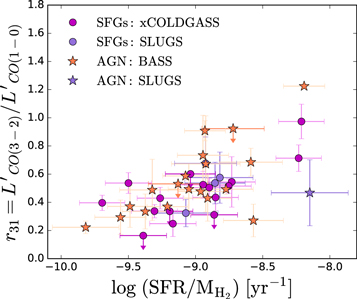
Figure 3. Ratio r31 =  /
/ as a function of SFE (SFE = SFR/M(H2)) for SFGs (circles) and AGN (stars). The SFG and AGN samples are matched in SSFR: at every SFG corresponds the AGN host galaxy with the most similar value of SSFR.
Download figure:
Standard image High-resolution imageMao et al. (2010) found a higher  in AGN than in normal SFGs (
 ). They however do not control for the SSFR, so it is possible that the difference in r31 is partly due to differences in SSFR between the two samples and not to the effect of the AGN. They also find higher r31 values in starbursts (
 ) and in ULIRGs (r31 = 0.96 ± 0.14) than in AGN. Additionally, most of the galaxies in their sample have rather large angular size (optical diameter D25 > 100'') and thus the CO beam is sampling a smaller region around the nucleus. Therefore, it is reasonable to expect that the AGN could have a large impact on the observed r31 line ratio.
We look at the relation between r31 and hard X-ray luminosity (14–195 keV) for the BASS sample, but we do not find a clear trend between the two quantities (see Figure 9 in the Appendix), which suggests that the X-ray flux is not the main parameter affecting this line ratio. Even though the X-ray radiation may contribute to enhance the r31 ratio in the nuclear region, as is shown later in Section 5.2, it is probably not enough to regulate the CO excitation in the entire galaxy.
We conclude that there is no significant difference between the values of r31 of AGN and SFGs.
5. Modeling: UCL-PDR
In order to better understand which physical parameters influence the line ratios r21 and r31, we model the CO emission lines using a photon-dissociation region (PDR) code. Our goal is to test which are the physical quantities that have the largest effect on the CO line ratios, and which values of these quantities can reproduce our observations.
We employ the 1D UCL-PDR code, developed by Bell et al. (2005, 2006) and upgraded by Bayet et al. (2011). The latest version of the code is presented in Priestley et al. (2017). The code models the gas cloud as a semi-infinite slab with a constant density, illuminated from one side by a far-ultraviolet (FUV) radiation field. At each depth point in the slab, the code calculates the chemistry and thermal balance of the gas self-consistently and returns, for every element, the gas chemical abundances, emission-line strengths, and gas temperature. Surface reactions on dust grains are not included.
The gas is cooled by the emission from collisionally excited atoms and molecules and by the interactions with the cooler dust grains (Bell et al. 2006). We include in our model the cooling from the following lines: Lyman α, 12C+, 12C, 16O, 12CO, and the para and ortho H2 and H2O states. Table 5 shows the elements included in the chemical network and their initial abundances relative to hydrogen, where depletion in the dust by some elements is already taken into consideration. For the values of the initial elemental abundances, we follow Bell et al. (2006). We set  (where
  is the volume density of hydrogen nuclei
 ) following Bell et al. (2005).
Table 5. Initial Elemental Abundances Used in the UCL-PDR Code Relative to the Hydrogen Nuclei
| Element | Abundance |
|---|---|
| He |

|
| O |

|
| C+ |

|
| N |

|
| Mg(+) |

|
| S(+) |

|
Download table as: ASCIITypeset image
We calculate the integrated line intensity of the CO emission lines as described in Bell et al. (2006). The opacity is included in the calculation of each coolant transition along each path (Bell et al. 2006; Banerji et al. 2009). The intensity I in units of erg s−1 cm−2 sr−1 is calculated by integrating the line emissivity Λ over the depth into the cloud L:

where Λ has units of erg s−1 cm−3, and the factor of 2π takes into account the fact that the photons only emerge from the edge of the cloud/slab.
The velocity-integrated antenna temperature in units of K km s−1 is calculated from the intensity as
where c is the speed of light, ν the frequency of the line, and kB is the Boltzmann constant.
The model is computed from AV = 0 to AV = 10. We choose the maximum AV value to be representative of the average visual extinction measured in dark molecular clouds. At these AV, the temperature is already ≤10 K and the gas enters the dense molecular cloud regime, where the freeze out starts to be efficient, and it can no longer be considered a PDR (Bergin & Tafalla 2007).
We define the r31 line ratio as the ratio between the integrated antenna temperatures:
where ν is the frequency of the line. In an analogous way, we calculated r21. This ratio is equivalent to the observed  luminosity ratio that we studied in the previous section.
5.1. CO Line Ratios from Modeling
We define a grid of models, varying three parameters: the volume density of hydrogen nuclei (
 ), the FUV radiation field, and the cosmic-ray ionization rate. The values assumed in our models are summarized in Table 6. The standard Galactic value of the cosmic-ray ionization rate is
  s−1 (Shaw et al. 2008). We select a range up to two orders of magnitude higher to take into account the fact that in AGN, the cosmic-ray density is higher (George et al. 2008 and references therein). Recent studies found that cosmic-ray ionization rates can be up to 100 times the Galactic value in particular regions of the interstellar medium (Indriolo & McCall 2012; Bisbas et al. 2015, 2017; Indriolo et al. 2015). Even though these extreme conditions may happen close to the source of cosmic rays, i.e., the AGN, the cosmic-ray ionization rate will decrease quickly with increasing H2 column density (Padovani et al. 2009; Schlickeiser et al. 2016). Because we are studying integrated CO fluxes within a beam that has a minimum size of ∼2 kpc, we do not expect to have an average cosmic-ray ionization rate higher than 10 times the Galactic value in the region covered by the CO beam.
Table 6. Parameters Used in the Grid of UCL-PDR Models
| Gas Density | FUV Radiation Field | Cosmic-Ray |
|---|---|---|
( ) ) |
(FUV) | Ionization Rate ( ) ) |
(cm
|
(Draine (a)) |
 s−1) s−1) |
| 102 | 10 | 2.5 (b) |
| 103 | 102 | 25 |
| 104 | 103 | 250 |
| 105 | ⋯ | ⋯ |
Note. (a) 1 Draine  erg s−1 cm−2. The FUV radiation is defined by the standard Draine field (Draine 1978; Bell et al. 2006). (b) Standard Galactic value (Shaw et al. 2008).
Download table as: ASCIITypeset image
We note that a limitation of our approach is the degeneracy of the low-J CO line ratios to the average state of the ISM (Aalto et al. 1995). Using only two low-J CO line ratios to derive physical properties of the gas can lead to large uncertainties. Additionally, it is possible that models with line ratios that match the observations have individual intensities that are unrealistic. We compare the individual line intensities from the UCL-PDR models which match the observed r31 line ratios, with the observed line intensities (both for CO(3–2) and for CO(1–0)). For all galaxies, we find that the line intensities from the models are higher than the observed line intensities (by a factor that varies between 1.7 and 124). This can be explained by beam dilution effects. The UCL-PDR models assume a 100% filling factor. The observed PDR regions typically do not fill the entire beam and thus the emission from the PDR regions is diluted when averaging over the beam. As a result, the observed intensities are lower than the ones predicted from the models. Even given these limitations, qualitatively the UCL-PDR models can provide an indication of which physical parameters have the highest impact in regulating the CO line ratios.
Figure 4 shows the modeled line ratios r21 (left) and r31 (right) as a function of  . The colors indicate different values of the FUV radiation field and different line types correspond to different cosmic-ray ionization rates. The parameter that has the largest effect on the line ratios is the density
  . As expected, there is a clear increase in both line ratios with
  . The r21 values are in the range 0.3–1.1. The r31 value goes from 0.01 at
  = 102 cm−3 to 1 at
  = 105 cm−3.

Figure 4. CO line ratios  (left) and
  (right) predicted from UCL-PDR as a function of gas density
  . The colors indicate models with different FUV values: 101 Draine (blue), 102 Draine (orange), 103 Draine (magenta). The line styles indicate models with different cosmic-ray ionization rates:
  s−1 (full line), 2.5 × 10⁻¹⁶ s−1 (dashed line), 2.5 × 10⁻¹⁵ s−1 (dotted–dashed line).
Download figure:
Standard image High-resolution imageThe FUV radiation field has very little effect on the line ratio. The only visible difference is for the r21 ratio: at  = 102 cm−3, it decreases from ∼0.45 for FUV = 10 Draine15
to ∼0.3 for FUV = 1000 Draine. At low density, the high FUV field suppresses the CO emission in all J levels. This is due to the fact that a stronger FUV field will increase the photodissociation of CO and consequently the CO abundance will decrease. The J = 2–1 level is slightly more suppressed than the J = 1–0 level, causing a decrease in the r21 line ratio.
= 102 cm−3, it decreases from ∼0.45 for FUV = 10 Draine15
to ∼0.3 for FUV = 1000 Draine. At low density, the high FUV field suppresses the CO emission in all J levels. This is due to the fact that a stronger FUV field will increase the photodissociation of CO and consequently the CO abundance will decrease. The J = 2–1 level is slightly more suppressed than the J = 1–0 level, causing a decrease in the r21 line ratio.
We note also that the cosmic-ray ionization rate does not have a big impact on the CO line ratios. We see an effect only at  = 104 cm−3, where there is an enhancement of ∼0.2 in both line ratios when the cosmic-ray ionization rate is two orders of magnitude above the Galactic value (2.5 × 10⁻¹⁵ s−1).
So, we conclude that both CO line ratios are mainly tracing the gas density. The range of variation of r21 is smaller than the range of r31, but it is still significant.
The mean r31 line ratio in the combined xCOLD GASS, BASS, and SLUGS samples is 0.55, which corresponds to a density of  ∼ 104 cm−3. We note that this value should be interpreted as the average gas density of the gas traced by CO, and not as the average gas density of the ISM in giant molecular clouds. The r21 value at that density from the UCL-PDR model is 0.8, which is consistent with the mean values reported by Saintonge et al. (2017) and Leroy et al. (2009).
One possible caveat of our analysis is that the FUV radiation field is modeled as the standard Draine field in the range 912–2000 Å, but the shape and intensity of the SED in the UV is different in AGN and in SFGs. This effect is not considered in our current model. However, we consider a wide range for the strength of the FUV field, in order to take into account the stronger UV field due to the accretion disk of AGN.
5.2. Effect of the X-Rays
We consider also the effect of the X-rays on the observed CO line ratios. AGN can be a strong source of X-rays, and this could potentially affect the excitation of the CO molecules. The BASS sample is selected in the hard X-rays, and therefore, we know that our sources are strong X-ray emitters.
The X-ray chemistry and physics are implemented in the latest version of the UCL-PDR code following Meijerink & Spaans (2005) and Stäuber et al. (2005). The shape and intensity of the X-ray spectrum can be defined to describe the spectrum of an AGN or of a young stellar object (Priestley et al. 2017). In the case of an AGN, the X-ray spectrum is modeled in the range 1–10 keV as a blackbody with a temperature of 1.16 · 107 K, corresponding to an energy kT = 1 keV. The intensity of the X-ray can be specified.
We estimate the X-ray flux that would be observed at a distance of 1 kpc from the AGN, based on the observed fluxes measured in the 2–10 keV energy band from Ricci et al. (2017). For our sample, this flux ranges from 10−4 to 3 × 10⁻¹ erg s−1 cm−2, with a median of 10−2 erg s−1 cm−2.
Figure 5 shows the modeled CO ratios r21 and r31 as a function of X-ray flux. For X-ray flux <10−2 erg s−1 cm−2 the effect on the CO ratios is negligible. This flux corresponds to an X-ray luminosity of ∼1042 erg s−1 in the 2–10 keV band, assuming that the flux is observed at 1 kpc from the nucleus. For higher X-ray fluxes in the range from 10−2 to 1 erg s−1 cm−2, both r21 and r31 are enhanced if they are combined with high densities ( cm−3). If instead they are combined with lower densities (
 cm−3), the ratios stay constant or decrease.

Figure 5. Predicted CO line ratios from UCL-PDR as a function of X-ray flux  of the left and
  on the right. The colors indicate models with different gas density values:
  = 102 cm−3 (green solid line), 103 cm−3 (blue dashed line), 104 cm−3 (red dotted–dashed line), and 105 cm−3 (magenta dotted line). For all models, the FUV radiation field is set at 100 Draine and the cosmic-ray ionization rate is set at the standard Galactic value
  s−1.
s−1.
Download figure:
Standard image High-resolution imageIf we consider an even higher X-ray flux of 10 erg s−1 cm−2 (corresponding to an X-ray luminosity of ∼1045 erg s−1), then the behavior is clearly different for high and low densities. For 
 cm−3, both line ratios decrease to
  and
and  . For the highest density considered
 cm−3, both line ratios increase to very high values (>3). This can be explained by the fact that for low-density gas, the high X-ray flux reduces the CO abundance, due to photodissociation of CO. Thus, the overall CO emission is weak, and the CO ladder peaks at J = 1. Only when the density is high enough can the X-rays start to excite the higher CO levels, causing the r21 and r31 levels to increase.
We conclude that the X-rays can affect the CO line ratios only for very high density and high X-ray flux. This is likely to occur only in a region very close to the active nucleus, but not in the rest of the galaxy. Thus, if we consider the total CO emission of a galaxy, we do not expect to see a difference due to the presence of an AGN.
6. Molecular Kennicutt–Schmidt Relation
In this section, we investigate how the relation between the SFR and the molecular gas mass changes when the latter is derived from the CO(3–2) luminosity instead of from the CO(1–0) luminosity. Because CO(3–2) is tracing only the denser gas, we expect that the KS relation (Kennicutt 1998) measured from CO(3–2) will be tighter. Past studies found that the CO(3–2) emission correlates more strongly than the CO(1–0) emission with SFR (Komugi et al. 2007; Muraoka et al. 2007; Wilson et al. 2009).
For this analysis we consider all properties measured within the beam, applying inverse beam corrections to scale the total SFR to the SFR measured within the beam. In this way we can also include the galaxies with large angular size ( ).
).
Figure 6 shows the KS relation with the total molecular gas mass measured from the CO(1–0) luminosity and the mass of the "dense" molecular mass measured from the CO(3–2) luminosity. The CO(3–2) luminosities have been converted to CO(1–0) luminosities using a constant r31 = 0.55 before applying the same CO-to-H2 conversion factor ( ) used for the CO(1–0) luminosities. We did not include in the fit the galaxies for which we used the "ULIRG-type"
  conversion factor (empty symbols in Figure 6). By assigning to them a different conversion factor, we implicitly assume that they have a different star formation mechanism and do not follow the same relation between the amount of molecular gas and the SFR. The correlation of SFR surface density with the molecular gas mass derived from CO(3–2) (measured by the Pearson correlation coefficient R = 0.84) is only slightly higher than the correlation with the molecular gas mass measured from CO(1–0) (R = 0.79). The two correlation coefficients are not significantly different, according to the Fisher Z-test (p-value = 0.06).
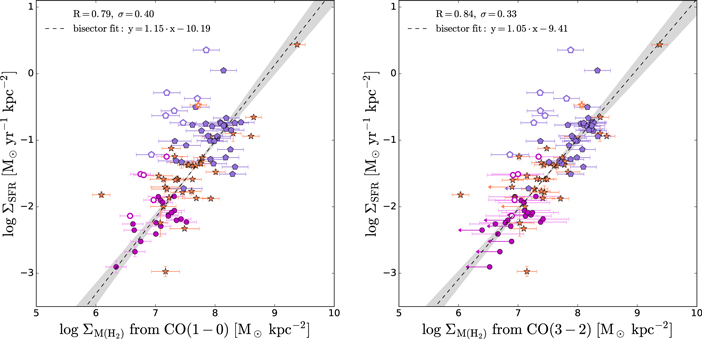
Figure 6. Kennicutt–Schmidt relation for the molecular gas measured from the CO(1–0) luminosity (left) and the molecular gas measured from the CO(3–2) luminosity (right). The CO(3–2) luminosities have been converted to CO(1–0) luminosities using a constant r31 = 0.55, before applying the same CO-to-H2 conversion factor ( ) as used for the CO(1–0) lines. The surface densities are calculated for the quantities within the telescope beams. The dashed line shows the ordinary least-squares bisector fit taking into account the upper limits. Circles are xCOLD GASS galaxies, the star symbol is used for AGN from BASS, and pentagons are galaxies from SLUGS. The empty symbols are the sources for which the "ULIRG-type" CO-to-H2 conversion factor (
 ) was used and which are not included in the fit.
Download figure:
Standard image High-resolution imageWe fit the KS relation  using the ordinary least-squares bisector fit (Isobe et al. 1990) taking into account the upper limits and including an intrinsic scatter. The fit to the molecular gas derived by CO(1–0) has a slope
  with an intrinsic scatter of 0.48, while the fit to the molecular gas derived by CO(3–2) gives a slightly lower value
  with intrinsic scatter 0.42. The two slopes are consistent with each other, within the uncertainties. We find that the KS relation becomes tighter when we consider only the dense molecular gas traced by the CO(3–2) transition. The intrinsic scatter decreases from 0.40 to 0.33, but it is still quite large also for the dense molecular gas. Thus, the fact that CO(1–0) is also tracing the diffuse molecular gas is probably not the only cause of the scatter in the KS relation. The CO(3–2) emission line is commonly used to measure the molecular gas content of galaxies at redshift
  , for which observations of the CO(1–0) line are more time consuming. Despite the fact that CO(3–2) is tracing denser gas than CO(1–0), the KS relations obtained from CO(3–2) and from CO(1–0) are similar, with slopes that are consistent with each other and similar scatters. It is important to note that we have excluded from this analysis the "ULIRG"-type of galaxies. The similar KS slope of CO(3–2) and CO(1–0) suggests that there is no systematic trend in SFE along the KS relation for "normal" SFGs in the parameter space studied in this paper. This result may not hold for objects above the main sequence (ULIRGs, starbursts), which have higher SFE with respect to main-sequence galaxies. For "normal" SFGs (with
  ), we do not observe a systematic variation of the mean r31 line ratio as a function of SFR (Figure 2). Thus, we do not expect systematic variations in the relation between the emission of "dense" and "total" molecular gas in these galaxies. Therefore, the KS relation derived from CO(3–2) can be directly compared to the KS relation derived from CO(1–0), once a constant offset due to the r31 line ratio is taken into account.
For galaxies with higher SFR ( ), the r31 ratio increases as a function of SFR. Thus, for galaxies above the main sequence, the systematic increase of the r31 values with SFR will cause the KS relation for CO(3–2) to be different from the CO(1–0) KS relation. Because we have excluded the ULIRG-type of galaxies from our analysis, this effect is not present in our result.
We also note that the SFE measured in our samples is similar to the SFE of main-sequence galaxies at higher redshift (z ∼ 1–3). For example, Aravena et al. (2019) find a typical depletion time of 1 Gyr (log SFE = −9) in galaxies with  , and Tacconi et al. (2013) find a mean depletion time of 0.7 Gyr, in a sample of galaxies at z ∼ 1–2.
Our result suggests that the CO(3–2) line can be used to study the relation between SFR and molecular gas for high-redshift "main-sequence" galaxies, and to compare it with studies of low-redshift galaxies.
7. Summary and Conclusions
In this paper, we study the ratio between the CO(1–0) and CO(3–2) emission of SFGs and AGN using observations and modeling.
Simulations from UCL-PDR show that the main parameter regulating the r31 ratio is the gas density. The FUV radiation field and X-rays play only a secondary role.
We find a relation between the r31 line ratio and the SFE using data from the xCOLD GASS, BASS, and SLUGS surveys. This relation was already reported for the full SLUGS sample by Yao et al. (2003), and in spatially resolved observations of M83, NGC 3627, and NGC 5055 (Muraoka et al. 2007; Morokuma-Matsui & Muraoka 2017). If the CO(1–0) emission traces the total molecular gas and the CO(3–2) emission traces the denser gas, then r31 can be interpreted as a measure of the fraction of molecular gas, which is in the dense star-forming molecular clouds. If this fraction is higher, then the efficiency of a galaxy in forming stars will be higher. The same effect is reflected in the tightening of the KS relation when we consider only the dense molecular gas, traced by CO(3–2), instead of the total molecular gas, traced by CO(1–0).
We have shown that the SFE is related to the amount of molecular gas which is in the dense phase, but we do not know which factors cause the variation of the dense molecular gas fraction. The presence of spiral arms and bars may be connected to a higher fraction of dense molecular gas (e.g., Sakamoto et al. 1999; Sheth et al. 2005). The presence of a bulge may also have an impact, with SFE that may be different in bulge or disk-dominated galaxies (Martig et al. 2009; Saintonge et al. 2012). However, we do not see a relation between r31 and the concentration index of the galaxies.
We also compare the r31 values in SFGs and active galaxies to test whether the presence of an AGN has an impact on the r31 ratio. We do not see a difference in the distribution of the r31 values of AGN and SFGs. This is not surprising, as the effect of the AGN is expected to become relevant at higher J levels (J > 10; Lu et al. 2017). The UCL-PDR models show that the X-rays emitted from an AGN can have an impact on the r31 values at higher gas density. However, the X-ray flux needs to be high ( erg s−1 cm−2) and thus the X-rays can affect the condition of the ISM only close to the nucleus. This explains why we do not see this effect if we consider the total CO emission of the host galaxy. This can be different at high redshift, where we can find both more luminous quasars (with bolometric luminosities
  erg s−1) and a higher fraction of dense gas. In these conditions, the presence of an active nucleus could significantly impact the r31 line ratio.
We do not find large variations in the r31 line ratio in our sample of "normal" SFGs. However, based on our modeling, we expect to observe higher r31 values in galaxies with a larger fraction of dense gas, as for example in starburst galaxies, ULIRGs, or in submillimeter galaxies at high redshift (e.g., Gao & Solomon 2004a; Carilli & Walter 2013; Riechers et al. 2013; Casey et al. 2014). If we were to study the r31 ratio in a sample of starbursts or ULIRGs, we would probably find different results. Indeed, Mao et al. (2010) found higher r31 in starburst and ULIRGs (0.89 ± 0.11 and 0.96 ± 0.14, respectively) than in normal star-forming galaxies (0.61 ± 0.16).
In summary, the main conclusions of this paper are:
- 1.The mean value of the r31 ratio in our sample is. There is no significant difference in the r31 values of SFGs and AGN.
- 2.We model the r31 using the UCL-PDR code and find that the main parameter regulating the r31 ratio is the gas density. The mean value corresponds to a volume density of hydrogen nuclei cm−3.
- 3.There is a trend for the r31 ratio to increase with SFE (p-value =). We find that the correlation with SFE is stronger than with SFR and SSFR.
- 4.The correlation of the KS relation increases when we consider molecular gas mass traced by CO(3–2) (R = 0.84), instead of the molecular gas mass traced by CO(1–0) (R = 0.79). However, the difference is not statistically significant (. This suggests that the CO(3–2) emission line can be used to study the relation between SFR and molecular gas for "normal" SFGs at high redshift and to compare it with studies of low-redshift galaxies.


We thank Felix Priestley for the help in installing and running the UCL-PDR code. A.S. acknowledges support from the Royal Society through the award of a University Research Fellowship. M.K. acknowledges support from NASA through ADAP award NNH16CT03C. E.T. acknowledges support from FONDECYT Regular 1160999, CONICYT PIA ACT172033, and Basal-CATA PFB-06/2007 and AFB170002 grants. This work is based on observations carried out with the IRAM 30 m telescope. IRAM is supported by INSU/CNRS (France), MPG (Germany), and IGN (Spain). The James Clerk Maxwell Telescope is operated by the East Asian Observatory on behalf of The National Astronomical Observatory of Japan; Academia Sinica Institute of Astronomy and Astrophysics; the Korea Astronomy and Space Science Institute; the Operation, Maintenance and Upgrading Fund for Astronomical Telescopes and Facility Instruments, budgeted from the Ministry of Finance (MOF) of China and administrated by the Chinese Academy of Sciences (CAS), as well as the National Key R&D Program of China (No. 2017YFA0402700). Additional funding support is provided by the Science and Technology Facilities Council of the United Kingdom and participating universities in the United Kingdom and Canada. The Starlink software (Currie et al. 2014) is currently supported by the East Asian Observatory. The Pan-STARRS1 Surveys (PS1) and the PS1 public science archive have been made possible through contributions by the Institute for Astronomy, the University of Hawaii, the Pan-STARRS Project Office, the Max-Planck Society and its participating institutes, the Max Planck Institute for Astronomy, Heidelberg, and the Max Planck Institute for Extraterrestrial Physics, Garching, The Johns Hopkins University, Durham University, the University of Edinburgh, the Queen's University Belfast, the Harvard-Smithsonian Center for Astrophysics, the Las Cumbres Observatory Global Telescope Network Incorporated, the National Central University of Taiwan, the Space Telescope Science Institute, the National Aeronautics and Space Administration under grant No. NNX08AR22G issued through the Planetary Science Division of the NASA Science Mission Directorate, the National Science Foundation grant No. AST-1238877, the University of Maryland, Eötvös Loránd University (ELTE), the Los Alamos National Laboratory, and the Gordon and Betty Moore Foundation. Funding for the SDSS and SDSS-II has been provided by the Alfred P. Sloan Foundation, the Participating Institutions, the National Science Foundation, the U.S. Department of Energy, the National Aeronautics and Space Administration, the Japanese Monbukagakusho, the Max Planck Society, and the Higher Education Funding Council for England. The SDSS Web Site is http://www.sdss.org/. The SDSS is managed by the Astrophysical Research Consortium for the Participating Institutions. The Participating Institutions are the American Museum of Natural History, Astrophysical Institute Potsdam, University of Basel, University of Cambridge, Case Western Reserve University, University of Chicago, Drexel University, Fermilab, the Institute for Advanced Study, the Japan Participation Group, Johns Hopkins University, the Joint Institute for Nuclear Astrophysics, the Kavli Institute for Particle Astrophysics and Cosmology, the Korean Scientist Group, the Chinese Academy of Sciences (LAMOST), Los Alamos National Laboratory, the Max-Planck-Institute for Astronomy (MPIA), the Max-Planck-Institute for Astrophysics (MPA), New Mexico State University, Ohio State University, University of Pittsburgh, University of Portsmouth, Princeton University, the United States Naval Observatory, and the University of Washington. This research has made use of the NASA/IPAC Extragalactic Database (NED), which is operated by the Jet Propulsion Laboratory, California Institute of Technology, under contract with the National Aeronautics and Space Administration. This research made use of Astropy, a community-developed core Python package for Astronomy (The Astropy Collaboration et al. 2013), Matplotlib (Hunter 2007), and NumPy (Van Der Walt et al. 2011). This research made use of APLpy, an open-source plotting package for Python (Robitaille & Bressert 2012). This research used the TOPCAT tool for catalog cross-matching (Taylor 2005). This research used the Stan interface for Python PyStan (Stan Development Team 2018).
Facilities: JCMT - James Clerk Maxwell Telescope, IRAM:30 m - .
Software: Astropy (The Astropy Collaboration et al. 2013), Matplotlib (Hunter 2007), NumPy (Van Der Walt et al. 2011), TOPCAT (Taylor 2005), PyStan (Stan Development Team 2018). Starlink (Currie et al. 2014).
Appendix
A.1. r31 Dependence on Galaxy Size and Beam Corrections
In order to check that the beam corrections and beam sizes do not have an effect on our analysis, we investigate if there is any relation between r31 and galaxy angular size. For the angular size of xCOLD GASS and SLUGS, we use  , i.e., the optical diameter from SDSS g band. For BASS, we use
  , where
  is the isophotal radius at 20 mag arcsec−2 in the K band. If there is a correlation between r31 and the galaxy angular size, that could mean that the part of the galaxy we are sampling is affecting the r31 measurements (i.e., the difference in the CO(1–0) and CO(3–2) beam sizes is affecting the r31 measurements.) For galaxies with large angular size, the telescope beam is only sampling a small part of the galaxy. If the gas is denser in the central part of the galaxy, r31 will be higher, and thus we expect to observe a higher r31 for galaxies with large angular sizes. On the other hand, if the region of the galaxy included in the beam is large enough, we would not find this trend. The left panel of Figure 7 shows r31 as a function of galaxy angular size. We do not find any trend of r31 increasing or decreasing with angular size (R = −0.03). Thus, we can rule out the possibility that the angular size plays a significant role in the r31 variations. We note that BASS objects have in general a larger angular size than the xCOLD GASS galaxies, due to their lower redshift (most objects in the BASS sample have
  with respect to
  for xCOLD GASS). We also look at the distribution of r31 with respect to the beam-correction factor
  (right panel of Figure 7). We do not see any evidence of r31 increasing with the beam-correction factor.
A.2. CO Spectra
Figure 8 shows the CO(3–2) spectra and SDSS gri images of the xCOLDGASS sample. Additional figures showing the remaining 15 galaxies of the xCOLDGASS sample and the full sample of 46 BASS objects are available as an online figure set.
A.3. r31 and X-Ray Luminosity
Figure 9 shows the r31 luminosity line ratio versus the hard X-ray luminosity (14–195 keV) for the BASS sample. We do not observe a clear correlation between r31 and the X-ray luminosity (Pearson correlation coefficient R = 0.33), suggesting that the X-ray luminosity does not contribute significantly in regulating this line ratio.

Figure 7. Left: ratio  as a function of galaxy angular diameter. For the angular diameter of xCOLD GASS and SLUGS, we use
  , i.e., the optical diameter from the SDSS g band. For the angular diameter of BASS, we use
  , where
  is the isophotal radius at 20 mag arcsec−2 in the K band. Right: ratio r31 as a function of the beam correction applied to account for the different beam sizes of the CO(3–2) and CO(1–0) beams. The beam corrections extrapolate the CO(3–2) flux to the area of the CO(1–0) beam.
Download figure:
Standard image High-resolution image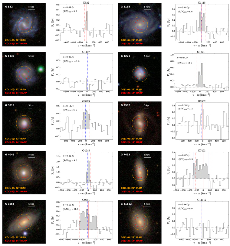
Figure 8.
Left: SDSS gri images of the xCOLD GASS sample. Every image has dimension 60'' × 60'' (1' × 1') and shows the size of the IRAM-30 m and JCMT HARP beams. Right: CO(3-2) spectra of the xCOLD GASS sample taken with HARP on the JCMT. The spectra are centred at the position of the CO(3-2) line. The solid red line is the central velocity of the line based on the spectroscopic redshift from SDSS and the dashed red lines indicate the interval where the CO(3-2) flux was integrated, based on the FWHM of the CO(1-0) line. The blue solid line indicates the central velocity of the CO(1-0) line. For the two galaxies (G7493 and G2527) where the CO(3-2) line flux was measured based on the position of the CO(1-0) line, the blue dotted line shows the interval where the CO(3-2) flux was integrated. Additional figures showing the remaining 15 galaxies of the xCOLDGASS sample and the full sample of 46 BASS objects are available as an online figure set. (The complete figure set (71 images) is available.)
Download figure:
Standard image High-resolution image
Figure 9. Ratio r31 =  /
/ as a function of hard X-ray luminosity measured in the 14–195 keV band for the BASS sample.
Download figure:
Standard image High-resolution image
Footnotes
- 11
- 12
- 13
- 14
- 15