


Abstract
The leading hypothesis for the origin of the Interstellar Boundary Explorer(IBEX) "ribbon" of enhanced energetic neutral atoms (ENAs) from the outer heliosphere is the secondary ENA mechanism, whereby neutralized solar wind ions escape the heliosphere, and after several charge-exchange processes, may propagate back toward Earth primarily in directions perpendicular to the local interstellar magnetic field (ISMF). However, the physical processes governing the parent protons outside of the heliopause are still unconstrained. In this study, we compute the "spatial retention" model proposed by Schwadron & McComas in a 3D simulated heliosphere. In their model, pickup ions outside the heliopause that originate from the neutral solar wind are spatially retained in a region of space via strong pitch angle scattering before becoming ENAs. We find that the ribbon's intensity and shape can vary greatly depending on the pitch angle scattering rate both inside and outside the spatial retention region, potentially contributing to the globally distributed flux. The draping of the ISMF around the heliopause creates an asymmetry in the average distance to the ribbon's source as well as an asymmetry in the ribbon's shape, i.e., a radial cross section of ENA flux through the circular ribbon. The spatial retention model adds an additional asymmetry to the ribbon's shape due to the enhancement of ions in the retention region close to the heliopause. Finally, we demonstrate how the ribbon's structure observed at 1 au is affected by different instrument capabilities, and how the Interstellar Mapping and Acceleration Probe may observe the ribbon.
Export citation and abstract BibTeX RIS
1. Introduction
The solar wind (SW) plasma emitted by the Sun interacts with the partially ionized gas of the very local interstellar medium (VLISM), creating the heliosphere (e.g., Zank 2015). While the SW and VLISM plasmas are separated at the heliopause (i.e., a tangential discontinuity), interstellar neutral atoms flow directly into the heliosphere and interact with the SW plasma via charge-exchange. This charge-exchange process produces energetic neutral atoms (ENAs) that can propagate in all directions, including toward Earth. The Interstellar Boundary Explorer (IBEX; McComas et al. 2009a), an Earth-orbiting spacecraft, observes interstellar neutral atoms, which allows us to determine the bulk properties of the VLISM (e.g., McComas et al. 2009b, 2015; Möbius et al. 2009, 2015; Zank et al. 2013; Bzowski et al. 2015; Schwadron et al. 2015, 2016; Sokół et al. 2015a; Swaczyna et al. 2015; Kubiak et al. 2016; Park et al. 2016), and it observes ENAs from the heliosheath (e.g., McComas et al. 2009b, 2014a, 2017; Dayeh et al. 2011, 2012, 2014; Schwadron et al. 2011, 2014; Reisenfeld et al. 2012, 2016; Desai et al. 2014; Zirnstein et al. 2014, 2016a, 2016b, 2017).
In 2009, IBEX discovered a band of enhanced ENAs, dubbed the "ribbon," forming a nearly complete circle in the celestial sky (McComas et al. 2009b). Its intensity is a few times brighter than the surrounding globally distributed flux. Schwadron et al. (2009) showed that the directions toward the ribbon are correlated with lines of sight perpendicular to the local interstellar magnetic field (ISMF) predicted by 3D global simulations of the heliosphere (Pogorelov et al. 2009). A number of mechanisms were proposed to explain the ribbon's origin, ranging from the inner heliosheath (IHS), the heliopause, and the outer heliosheath (OHS) region just outside the heliopause (McComas et al. 2009b). Since then, more possibilities have been suggested (for a review, see McComas et al. 2014b; see also Isenberg 2014; Giacalone & Jokipii 2015; Zirnstein et al. 2018).
Charge-exchange is a ubiquitous process occurring throughout the heliosphere, creating multiple, non-thermalized populations of pickup ions in different regions of space (e.g., Zank 1999, 2016; Malama et al. 2006). In this study we define new terminology that we suggest can be adopted to distinguish several populations of pickup ions that are commonly referred to, but usually not distinguished by name, in the literature.
As the neutral interstellar wind flows into the heliosphere, interstellar neutral atoms may charge-exchange with SW ions. The ionized neutral atoms are "picked up" by the SW, which we refer to as "pickup ions from neutral interstellar wind," or PINI. The neutralized SW ions become ENAs that propagate radially away from the Sun and almost all escape the heliosphere due to the low probability of ionizing inside the heliosphere. However, the OHS is ∼50 times denser than the IHS, making it likely that ENAs will ionize within a few hundred astronomical units of the heliopause. These ENAs that propagate outside the heliosphere and charge-exchange in the OHS become ions that gyrate around the ISMF (we refer to these ions as "pickup ions from neutral solar wind," or PINS). Within a few years, these PINS will charge-exchange again with interstellar neutral atoms, creating secondary ENAs that may travel back toward Earth and be detected by IBEX as the ribbon flux. An illustration of this process is shown in Figure 1. After over seven years of evolving ENA observations of the ribbon from IBEX, McComas et al. (2017) argued that the "IBEX observations strongly support a secondary ENA source for the ribbon," and suggested that it "be adopted as the nominal explanation of the ribbon going forward." However, the dynamical behavior of the PINS before they become secondary ENAs, in particular the evolution of their pitch angle distribution in space, is still poorly understood.
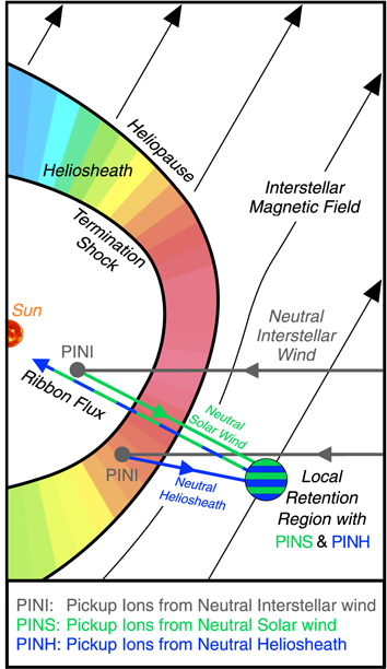
Figure 1. Illustration of the processes involved in creating ribbon flux from the spatial retention model. The neutral interstellar wind flows into the heliosphere, creating PINI in the solar wind and in the heliosheath. The neutral solar wind and neutral heliosheath atoms escape the heliosphere and ionize in the VLISM, creating PINS and PINH, respectively. PINS and PINH created in the retention region can, after another charge-exchange, propagate back toward Earth and be detected by IBEX. Note that in this study, we do not include ribbon fluxes created from PINH. The background color in the heliosheath represents globally distributed ENA fluxes observed by IBEX in early 2018. Adapted from McComas et al. (2019).
Download figure:
Standard image High-resolution imageThere are two general scenarios that have been suggested to explain the transport of PINS outside of the heliopause. (1) PINS experience negligible pitch angle scattering, such that only PINS that were created with and maintained large pitch angles, in radial directions ( ) nearly perpendicular to the ISMF (
 ), i.e.,
  , can become secondary ENAs observable at 1 au (Chalov et al. 2010; Gamayunov et al. 2010, 2017; Heerikhuisen et al. 2010; Möbius et al. 2013; Zirnstein et al. 2013, 2015a; Giacalone & Jokipii 2015). (2) PINS experience strong pitch angle scattering either due to self-generated waves or existing Alfvénic turbulence (e.g., Florinski et al. 2010), resulting in nearly isotropic pitch angle distributions in regions of space near
  (Schwadron & McComas 2013; Isenberg 2014). The "spatial retention" model (Schwadron & McComas 2013) is distinctly different from velocity retention models (e.g., Heerikhuisen et al. 2010), since it is inherently assumed that PINS will significantly scatter in pitch angle in a physical region of space near
  (i.e., the retention region) before they become ENAs, and are not required to maintain5
their initial pitch angles over long periods of time.
(i.e., the retention region) before they become ENAs, and are not required to maintain5
their initial pitch angles over long periods of time.
Recent developments in particle-in-cell simulations of PINS outside the heliopause suggest that PINS could maintain their highly anisotropic distribution over a period of time longer than previously thought (Florinski et al. 2010), depending on the thermodynamic properties of the OHS plasma (Florinski et al. 2016). However, Florinski & Heerikhuisen (2017) suggested that this may become complicated when considering another contribution of energetic ions, i.e., "pickup ions from the neutral heliosheath," or PINH, as their large thermal energies may drive a narrow pitch angle distribution unstable. Note that we do not include PINH as a source for the ribbon in this study.
The aim of this study is to improve our understanding of the physical processes controlling the PINS distribution outside of the heliopause by modeling the ribbon in a 3D MHD/kinetic simulation of the heliosphere. In a recent paper, Zirnstein et al. (2018) modeled the 3D ribbon under the limit of weak pitch angle scattering. In this study, we apply the physical dynamics in the strong pitch angle scattering limit proposed by Schwadron & McComas (2013; hereafter referred to as SM13) to model the ribbon. In the following sections, we describe the heliosphere simulation and ribbon model, present our results, and discuss physical characteristics that can be used to deduce the origin of the IBEX ribbon.
2. Model
2.1. Simulation of the Heliosphere
We utilize the results from a global simulation of the SW-VLISM interaction (Zirnstein et al. 2016b). This simulation is based on a 3D plasma-neutral code that iteratively solves magnetohydrodynamic (MHD) equations for the single-fluid plasma and Boltzmann's equation for neutral hydrogen atoms. The plasma and neutrals are coupled via energy-dependent, charge-exchange source terms (see, e.g., Pogorelov et al. 2008). The VLISM outer boundary conditions at 1000 au from the Sun are chosen based on values determined when constraining the IBEX ribbon by (1) Zirnstein et al. (2016b) for the ISMF magnitude of 2.93 μG and (2) McComas et al. (2015) for the interstellar neutral temperature of 7500 K (assumed to be the same for ions), and the interstellar flow speed of 25.4 km s−1 from inflow direction (255 7, 51) in ecliptic J2000 coordinates. The ISMF direction imposed at the simulation outer boundary is (22728, 3462), which is determined from the IBEX ribbon geometry by Zirnstein et al. (2016b), it lies on the hydrogen deflection plane (Lallement et al. 2010), and it produces a draped magnetic field around the heliopause consistent with Voyager 1 observations.
The VLISM boundary conditions are also chosen such that the model reproduces (1) the distance to the heliopause in the Voyager 1 direction (Gurnett et al. 2013), (2) the average ribbon center and structure (Funsten et al. 2013), (3) the consistency of the interstellar neutral hydrogen deflection plane and B–V plane (Lallement et al. 2010), and (4) the interstellar neutral hydrogen density at the termination shock near the VLISM inflow direction (∼0.1 cm−3; Bzowski et al. 2009). It is believed that Voyager 2 crossed the heliopause in November 2018 at a distance of ∼119 au from the Sun (see footnote 5). The heliopause can move in response to changes in the SW and our steady-state heliosphere simulation does not account for these changes. Nonetheless, the distance to the heliopause in the direction of Voyager 2 in our simulation is ∼120 au, generally consistent with Voyager 2 observations.
The SW boundary conditions at 1 au are the same as those used by Zirnstein et al. (2016b): the SW plasma density is 5.74 cm−3, the temperature is 51,100 K, the flow speed is 450 km s−1, and the magnetic field radial component is 37.5 μG. These values are advected to the simulation's inner boundary at 10 au by applying Parker's solution for the SW. The MHD and kinetic-neutral modules are iteratively solved until a steady state is achieved. We note that while our choice of SW boundary conditions as being latitude-independent are not valid at times near solar minimum, in the following section we impose a model that accounts for the latitudinal structure of the neutralized SW.
We note that the main results presented in this study are not significantly sensitive to the simplified SW boundary condition parameters imposed in the heliosphere simulation. The SW boundary conditions are assumed to be static in time, which is not realistic. Variations in the SW dynamic pressure can cause changes in the heliosphere boundary distances (e.g., McComas et al. 2018b, 2019) and may introduce changes in the ribbon source. However, since the ribbon source is extended over tens to hundreds of astronomical units, small fluctuations in the heliopause (a few astronomical units) are not expected to affect the main results of this study, such as the spatial structure of the ribbon source. Uncertainties in the neutralized SW distribution, which we analytically construct as the source of PINS outside the heliopause (see Section 2.2), may also affect the ribbon ENA intensity by an amount proportional to the neutral flux, but it will not significantly affect the ribbon's source structure. The VLISM boundary conditions are constrained using multiple spacecraft data sets and small uncertainties in their values are not expected to significantly affect the results.
2.2. Model of the Neutralized SW
It is important for this study to generate as realistic as possible a neutral hydrogen distribution originating from the supersonic SW to model a spatial retention-generated ribbon. The neutral hydrogen source terms from our kinetic-neutral module are computed using statistics from individual charge-exchange events, accumulated on a Cartesian grid. These results are then used to create a 6D phase space distribution for neutral hydrogen in the heliosphere, with an angular resolution of 6° (e.g., Heerikhuisen et al. 2016), which we can use to compute ENA generation in the heliosphere. However, to better simulate the very narrow width of the neutralized SW (see, e.g., Florinski & Heerikhuisen 2017), in this study we artificially generate a neutralized SW distribution following Swaczyna et al. (2016b), who demonstrated the dependence of the ribbon's position in the sky with the energy-dependent, latitudinal structure of the SW.
Here, we summarize the methodology of creating a neutralized SW distribution from Swaczyna et al. (2016b). We utilize a model of the SW speed and density as a function of latitude derived from interplanetary scintillation (IPS) observations (Sokół et al. 2015b). Since the delay between SW observations at 1 au and IBEX ribbon observations is expected to be ∼4–9 yr (Zirnstein et al. 2015b), we average SW data (speed up,0 and density np,0) over time periods that emulate the time-averaging inherent in the line-of-sight integration of ENAs outside the heliopause. The neutralized SW differential flux, INSW, at the termination shock, rTS, is given by Swaczyna et al. (2016b)
where v is the neutral SW speed, θ is the heliolatitude, i is the Carrington rotation number out of total M which we average over (see specific time periods below), np,0 and up,0 are the SW density and speed at 1 au, nH is the interstellar neutral hydrogen density in the supersonic SW, σex is the energy-dependent, charge-exchange cross section from Lindsay & Stebbings (2005), r is the distance from the Sun over which we integrate from r0 = 1 au to the termination shock (rTS = 100 au), and N is a Gaussian speed distribution with mean speed up,i(r) and thermal speed δv = 100 km s−1, which we use to smooth the SW distribution, similar to Swaczyna et al. (2016b). The SW speed up slows down due to mass-loading of injected PINI, which is approximated by (e.g., Lee et al. 2009; Swaczyna et al. 2016b)
where γ = 5/3, nH = 0.09 cm−3 (Bzowski et al. 2009), nHe = 0.015 cm−3 (Gloeckler et al. 2004), and νH and νHe are the photoionization rates for hydrogen and helium atoms, respectively, at 1 au.
Since the photoionization rates are significantly smaller than the neutral hydrogen charge-exchange rate, we assume νH and νHe are both constant, with values of 10−7 s−1 (Bzowski et al. 2013; Sokół et al. 2019). We integrate Equation (1) to a characteristic distance to the termination shock (rTS = 100 au), producing neutralized SW fluxes at the termination shock similar to those presented by Swaczyna et al. (2016b).
The neutral SW differential flux at the termination shock is shown in Figure 2 for different time periods that correspond to times expected to influence IBEX ENA observations of the ribbon (McComas et al. 2017). For typical delay times of ∼4–9 yr for secondary ENAs with energies between 1 and 4 keV, IBEX observations of the ribbon over the first three years (2009–2011) approximately correspond to SW properties over the period 2000–2007. Ribbon observations in 2011–2013 correspond to a SW period of 2003–2009, and so on. As shown in Figure 2, there is an enhancement in flux at low latitudes (<30°) and low energies (<1.5 keV) due to the low-latitude, slow SW. At energies above ∼1.5 keV, the dominant SW flux expands to higher latitudes, which, during solar minimum, emanate from the polar coronal holes. Moreover, there is a noticeable change in the SW flux over time, with a general decrease from ∼2000 to 2013 due to the relatively weak solar cycle 23 (McComas et al. 2013).
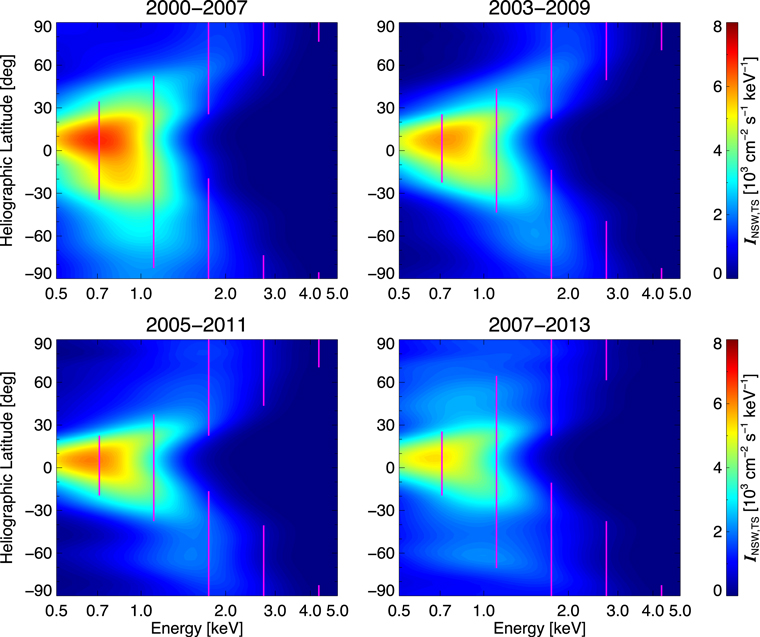
Figure 2. Neutral SW flux INSW at the termination shock (assumed to be 100 au) as a function of energy and heliographic latitude. The images show averages over four different time periods that correspond to IBEX ribbon observations from 2009 to 2011 (top left), 2011 to 2013 (top right), 2013 to 2015 (bottom left), and 2015 to 2017 (bottom right). The vertical magenta lines show the ranges of heliographic latitude corresponding to the central energies of the IBEX-Hi energy channels, where the lines correspond to values that are higher than half of the maximum.
Download figure:
Standard image High-resolution imageFor the main results in this paper (Section 3), we simulate the IBEX ribbon using SW properties averaged over 2000–2009, which can be compared with the 5 yr ribbon-separated observations derived by Schwadron et al. (2014). A more self-consistent, time-dependent comparison between our model and IBEX data over the first 9 yr of IBEX observations (Schwadron et al. 2018) will be performed in a future study.
2.3. Ribbon Model—Spatial Retention with Pickup Ion Enhancement
We briefly summarize the ribbon model developed by SM13 and implemented in this study. The PINS distribution inside the retention region (where the PINS initial parallel speed v∥ is less than the local Alfvén speed vA) is approximately given by

where SNSW is the neutral SW source rate (in units of s2 cm−6), 1/τx = nH( )σex(v)v is the charge-exchange rate, nH is the local interstellar neutral hydrogen density derived from the MHD-kinetic simulation, and
  is the three-dimensional position vector. The variable z is the distance along the local ISMF line away from the center of the retention region (
 ), and zA defines the boundary of the retention region where the local Alfvén speed vA is equal to the PINS parallel speed. For simplicity, we assume that the magnetic field line near the retention region is locally planar, such that z = r × tan[π/2 − α], where r is the distance from the Sun and α is the PINS initial pitch angle.
The neutral SW source rate is given by

The neutral SW differential flux INSW( ) changes as a function of distance r from the Sun due to (1) the r−2 expansion of the neutral SW and (2) the loss by charge-exchange in the OHS. Assuming that the neutral SW's thermal temperature is insignificant, the flux outside of the heliopause is
where np is the OHS plasma density extracted from our MHD-kinetic simulation and r' is the radial distance from the heliopause.
The function f (z ≤ zA) in Equation (3) describes the balance between the supply of ions into the retention region and the loss of particles by escape. The solution inside the retention region is (see the appendix in SM13)
the amplitude a is
the wavenumber k± is
the frequencies ν1 = 1/τ1 and νS = 1/τS are related by

and τs is the mean scattering time. The scattering time is calculated using the pitch angle diffusion coefficient, Dμμ. Following SM13, we use Dμμ from the case for gyro-resonant scattering of particles from field-aligned propagating Alfvén and fast magnetosonic waves (e.g., Schlickeiser 1989). For a prescribed isotropic Kolmogorov power spectrum  , the pitch angle diffusion coefficient is given by (e.g., Gamayunov et al. 2010)
where (Bslab/B)2 is the ratio of the slab component magnetic energy to the background magnetic energy, Ωp = qB/mp is the proton gyrofrequency, lb = 2π/kmin is the critical wavelength separating the energy-containing range from the inertial range, and v is the particle speed. Similar to SM13, we present results for the case where (Bslab/B)2 = 0.01 and lb = 0.005 au. The scattering time τs is related to Dμμ by the parallel spatial diffusion coefficient (e.g., Jokipii 1966; Hasselmann & Wibberenz 1970)
where λ∥ is the parallel mean free path and κ∥ is the spatial diffusion coefficient. Rather than assuming Dμμ ∼ Dμμ(μ = 0) as in SM13, we compute τS directly using Equations (11) and (12). Outside the retention region, the rate of turbulent scattering (1/τS) is assumed to be significantly weaker than that inside the retention region, thus outside we assume τS is much larger than the PINS-to-ENA charge-exchange time, τX (or 1/τS ≪ 1/τX). However, in Section 3.3 we relax this assumption to understand how different scattering rates outside the spatial retention region affect the ribbon flux observed at 1 au.
For the PINS distribution outside of the retention region, only the hemisphere propagating inward toward the retention region can produce ENAs observable at 1 au, which are populated by charge-exchange sources only, such that

For more details on the model derivation and assumptions, see SM13. However, note that the main difference between our model calculations and that of SM13 is that we solve their model equations using plasma and neutral properties from our 3D MHD-plasma and kinetic-neutral simulation of the heliosphere (Zirnstein et al. 2016b). Thus, we use our MHD-derived plasma density, flow speed, temperature, magnetic field, and neutral hydrogen distribution to compute ribbon ENA fluxes (see Section 2.5).
2.4. Ribbon Model—Isotropic Scattering
We also present a model of the ribbon whereby PINS immediately isotropize in pitch angle before creating secondary ENAs, forming an isotropic shell distribution at speed v. This model is similar to that presented by Heerikhuisen et al. (2014) and was demonstrated to produce too few ENAs. However, we present this model because of the different ribbon shape it produces compared to the spatial retention model (see Section 3.4).
For this model, similar to SM13, we assume that strong scattering occurs inside the spatial retention region where the initial PINS parallel speed is less than the local Alfvén speed. Unlike Heerikhuisen et al. (2014), however, we assume that PINS generated outside of the spatial retention region (v∥ > vA) do not experience significant pitch angle scattering. Since these PINS are traveling with velocities away from the retention region, they do not generate ENAs directed back toward Earth. The only PINS that can produce observable ENAs, under this model assumption, are those created inside the retention region. Thus, the distribution function for PINS inside and outside the retention region is given by, respectively,

2.5. ENA Model
Similar to our previous work (see, e.g., Zirnstein et al. 2018 and references therein), we compute ENA fluxes at 1 au by numerically integrating the differential flux equation given by
where Ω represents the angular direction from which the ENAs are coming, f0 is the PINS distribution inside (Equations (3) or (13)) or outside (Equations (12) or (13)) the retention region, rHP is the distance to the heliopause, and rOB is the distance to our model's outer boundary (here we set rOB = 700 au). We account for the ENA survival probability, P( , v), from its point of creation to the SW termination shock (∼100 au), but ignore their losses as they travel from the termination shock to 1 au, making our results directly comparable with survival probability-corrected IBEX ENA data (e.g., Figure 9 of McComas et al. 2017). We integrate Equation (14) over a range of ENA speeds corresponding to the IBEX-Hi energy ranges and integrate over the IBEX-Hi energy response functions (Funsten et al. 2009). Finally, when constructing the all-sky maps, we apply an angular smoothing algorithm that mimics the IBEX-Hi angular collimator response (Funsten et al. 2009). Note that this can significantly change the shape of the ribbon observed by IBEX at 1 au, as we demonstrate in Section 3.4.
3. Results
3.1. ENA All-sky Maps
Figure 3 shows the results of the spatial retention and isotropic scattering models presented in Section 2, alongside ribbon-separated IBEX-Hi data from the first five years of observations (Schwadron et al. 2014). We show results at 1.1 and 2.7 keV for which the ribbon is the most pronounced at the mean energies of the slow and fast SW. At 1.1 keV, the model and data show a single ribbon structure, which is a reflection of the neutralized slow (∼350–450 km s−1) SW at low to mid latitudes. At 2.7 keV, the ribbon breaks into two lobes because ∼2.7 keV PINS outside the heliopause originate from the neutralized fast (>650 km s−1) SW at high latitudes. This behavior is also seen in the observations. As one can see, there are clear differences in the overall intensities of the data and models. The spatial retention model produces approximately 3 times more ENAs than the isotropic scattering model due to the enhanced PINS density inside the retention region. However, depending on the energy and direction in the sky, the spatial retention model fluxes can be up to ∼1.5–3 times lower than IBEX data.
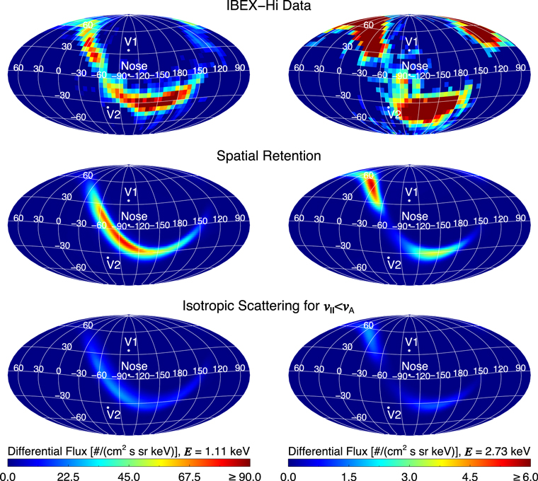
Figure 3. All-sky maps of IBEX-Hi ribbon-separated data from Schwadron et al. (2014) (top) and model results (middle, bottom) of ribbon ENA fluxes at 1.11 keV (left) and 2.73 keV (right). For the spatial retention model, we assume the rate of pitch angle scattering, 1/τs, outside the spatial retention region is much smaller than the rate of charge-exchange, 1/τx.
Download figure:
Standard image High-resolution imageDepending on the pitch angle scattering rate, the spatial retention model can also produce a diffuse background of ENA fluxes away from the spatial retention region (not shown in Figure 3), which may contribute to the globally distributed fluxes observed by IBEX. This is due to the backward-propagating hemisphere of the PINS distribution (Equation (13)). We demonstrate this later in Section 3.3.
Besides the amplitudes being significantly different, the shape of the ribbon is slightly different between the two ribbon models, although this is not obvious from Figure 3. The ribbon is slightly wider and slightly farther away from the nose of the heliosphere in the isotropic scattering case, both at 1.1 and 2.7 keV. These shapes, which are due to where the ENAs are coming from and their concentration as a function of angle away from  , may be able to provide us a means to differentiate between secondary ENA ribbon models, either using IBEX or future Interstellar Mapping and Acceleration Probe (IMAP) observations (McComas et al. 2018a). This is analyzed in more detail in Section 3.4.
3.2. Ribbon Source Region
To better understand where these ENAs are coming from as a function of spatial location, in Figure 4 we show the average distance to the ribbon ENA source region in the entire sky, specifically the distance at which 50% of the ENA flux is line-of-sight integrated starting from the heliopause. It is clear that the distance to the ribbon source changes significantly from the inner to the outer edges of the ribbon (for similar results, see also Heerikhuisen & Pogorelov 2011). In the inner part of the ribbon, closest to the nose direction of the heliosphere, the average distance to the ribbon source is ∼120–150 au. At the outer edge, the average distance increases to >300 au. This asymmetry, which is similar at different ENA energies and independent of the different ribbon models, is due to the draping of the ISMF around the heliosphere and specifically the location of  as seen in Figure 5.

Figure 4. All-sky maps showing distances to the ribbon source for the spatial retention (top) and isotropic scattering (bottom) models. Pixels with flux <10% of the maximum in the sky are colored gray.
Download figure:
Standard image High-resolution image
Figure 5. Meridional cuts through the nose of the heliosphere of the model ENA ribbon production rate at 1.11 keV (left) and 2.73 keV (right) for the spatial retention model (top) and the isotropic scattering model (bottom). Note that we only show ENA fluxes that are visible at 1 au by IBEX.
Download figure:
Standard image High-resolution imageFigure 5 shows the ribbon ENA production rate (in log10 scaling) in a meridional cut through the SW-VLISM interaction. The production rate, similar to that shown in Zirnstein et al. (2015a), is related to the fluxes shown in Figure 3 by integrating the flux as a function of radial distance from the heliopause outward. Note that the fluxes shown in Figure 5 are only those contributing to fluxes visible at 1 au. As one can see, the strongest emissions from the ribbon source region are closest to the heliopause due to (1) the r−2 expansion of the neutralized SW and (2) their loss due to charge-exchange as they travel through the relatively dense OHS. It is also clear that, due to the draping of the ISMF (see Pogorelov et al. 2011; Zirnstein et al. 2016b), the ribbon source region "bends" away from the radial direction at greater distances from the heliopause. This bending creates a natural width to the ribbon viewed from Earth, but also creates the asymmetry in the source distance shown in Figure 4. For example, at x = 120 au and z = −50 au, the ribbon source creates emissions seen at 1 au at relatively low latitudes near the ecliptic plane (i.e., the inner edge of the ribbon). However, at large (negative) z (x = 300 au, z = −300 au), this source contributes to pixels at higher (negative) latitudes (i.e., the outer edge of the ribbon).
Interestingly, the spatial retention and isotropic scattering models produce significantly different source structures. The spatial retention model creates a narrow peak in emission centered at  (red fluxes in the top left panel of Figure 5) and decreases farther from
  . Outside the retention region (when v∥ > vA), there is very little emission due to the assumption of low pitch angle scattering rates (see Section 3.3 for more details). The isotropic scattering model, which assumes at each location in the retention region the newly born PINS quickly scatter onto an isotropic shell distribution, creates uniform emission in the retention region. These differences in emission as a function of source location are very important for the ribbon shape observed at 1 au (see Section 3.4).
3.3. Pitch Angle Scattering Rate outside the Retention Region
In this section we change the rate of pitch angle scattering outside the retention region to understand its effect on the ribbon flux visible at 1 au. Specifically, in Equation (12), we assume either that (1) 1/τs (the pitch angle scattering rate) is significantly smaller than 1/τx (the charge-exchange rate), similar to the results shown in the previous sections, or (2) 1/τs ≫ 1/τx, implying that pitch angle scattering is significantly faster than the charge-exchange production/loss rate. The ribbon sky maps and average source distances are shown in Figures 6 and 7, and their production rates are shown in Figure 8. By assuming the pitch angle scattering rate is large outside the retention region, more ENAs from outside the retention region can scatter into backward-propagating hemispheres and be visible at 1 au, creating a smooth transition from inside to outside the retention region. At 1 au, this effectively creates a background of emissions away from the nominal ribbon position. This amount of flux could potentially contribute a significant number of ENAs to the globally distributed fluxes observed by IBEX. At ∼1 keV, this diffuse background is strongest at low latitudes near the nose of the heliosphere due to (1) the low-latitude, slow (∼1 keV) neutral SW, (2) larger interstellar plasma/neutral densities near the nose of the heliosphere, and (3) smaller distances to the heliopause (see Figure 8). At ∼3 keV, the background flux emanates from directions closer to the solar poles due to the high-latitude, fast (∼3 keV) neutral SW, but shifted toward the noseward hemisphere due to the larger interstellar densities and closer heliopause.

Figure 6. Model all-sky maps of ribbon ENA fluxes at 1.11 keV for the spatial retention model, assuming (top) the pitch angle scattering rate 1/τs ≪ 1/τx, the charge-exchange rate, outside the retention region, and (bottom) 1/τs ≫ 1/τx. The scattering rates inside the retention region are the same for both cases. In the right panels we show the average distance to the ribbon's source, similar to Figure 4.
Download figure:
Standard image High-resolution image
Figure 7. Similar to Figure 6, except for ribbon ENA fluxes at 2.73 keV.
Download figure:
Standard image High-resolution image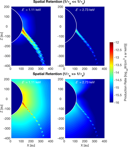
Figure 8. Meridional cuts through the nose of the heliosphere of the model ENA ribbon production rate at (left) 1.11 keV and (right) 2.73 keV for the spatial retention model results shown in Figures 6 and 7.
Download figure:
Standard image High-resolution imageNote that the fluxes in the direction of the ribbon in Figures 6 and 7 also increase when the pitch angle scattering rate is increased outside the retention region, which is due to the fact that the ribbon source region bends as a function of distance from the heliopause. Specifically, in any particular direction toward the ribbon, ENAs are being created from both within the local retention region, but also at other distances along the same line of sight there are some ENAs being created from the backward-propagating hemisphere from outside the retention region. Thus, the draping of the ISMF creates a curvature in the  surface and allows more ENAs to be visible at 1 au than is expected (at least compared to the case when 1/τS ≪ 1/τX). The overall intensities of these results compare more favorably to IBEX data.
3.4. Ribbon Shape and Instrumental Effects
An important aspect required to determine the origin of the ribbon is first understanding how the detector's angular response affects the observed ribbon fluxes at 1 au. In the previous sections, we simulated the IBEX angular response (Funsten et al. 2009), which tends to smooth sharp features in the sky that are on the order of ∼7° or smaller. Since the ribbon's true width could be <20° wide (Fuselier et al. 2009), the IBEX-Hi instrument is likely smoothing and widening the ribbon. Thus, in this section, we demonstrate how including or excluding the IBEX angular instrument response can affect the shape of the ribbon at 1 au, i.e., the radial cross section of ENA flux through the circular ribbon. We also model the expected IMAP-Hi instrument response (McComas et al. 2018a).
For this analysis, we first transform the model results into a ribbon-centered frame originally defined by Funsten et al. (2013). For simplicity we only show model results at an ENA energy of 1.1 keV. Based on the updated fitting results found by Dayeh et al. (2019), we rotate the model sky map to be centered on ecliptic J2000 (21964, 4147), which these authors found to be the best-fit center of the observed 1.1 keV ribbon flux over the time period 2009–2017. The resulting ribbon-centered maps are shown in the top panels of Figure 9. Note that we assume the center of our model ribbon is the same as that of the IBEX ribbon from Dayeh et al. (2019). This assumption is satisfactory for our qualitative analysis but will be validated in a future study.
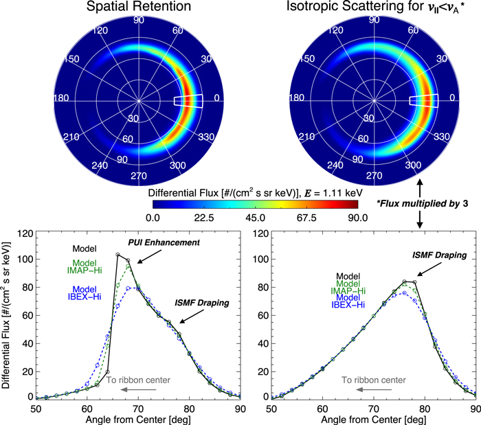
Figure 9. (Top) Ribbon-centered polar plots of ENA fluxes at 1.11 keV for the spatial retention model where 1/τs ≪ 1/τx (left) and the isotropic scattering model (right). Note that we multiply the isotropic scattering fluxes by a factor of 3 to show it on the same scale as the other model results. (Bottom) Model ribbon ENA fluxes as a function of angle from the polar plot center. Fluxes are extracted from the pixels shown within the white contour in the top panels, averaged along the azimuthal direction. We show model fluxes without any instrument angular response (black), with the IBEX-Hi angular response (blue), and with the IMAP-Hi angular response (green). Note that all prior model ENA fluxes shown in this paper, including the top panels here, were calculated using IBEX-Hi's angular response.
Download figure:
Standard image High-resolution image
In the bottom panels of Figure 9 we show the ribbon flux as a function of angle from the center, averaged over azimuthal pixels within ±6° of the 0° azimuth line (white boxes). We smooth the all-sky ribbon flux using a triangular function with an FWHM of 7° to approximate the IBEX-Hi collimator response (FWHM ∼65; Funsten et al. 2009), and an FWHM of 4° to emulate the IMAP-Hi response (McComas et al. 2018a). We also show results where there is no smoothing. Clearly, there are unique differences in how the instrument responses change the ribbon profile for each model. For the spatial retention model, the result without any instrument response is sharply peaked at ∼66° from the center, with a steep slope toward the center and gradual slope away from the center, creating a highly non-Gaussian shape. Interestingly, this asymmetry in the ribbon's flux profile is opposite that of the asymmetry calculated from IBEX-Hi data by Funsten et al. (2013), who found a steeper slope on the ribbon's outer edge (see their Figure 7). When we include the IBEX-Hi instrument response in the calculation, the ribbon appears more Gaussian-like and the peak of the ribbon lies closer to ∼69° away from the center, but the asymmetry is still present. The IMAP-Hi model better resolves the asymmetric shape of the ribbon and yields a ribbon peak at ∼68°. We also note that IMAP will have significantly better statistics than IBEX, providing a much better determination of the ribbon's shape.
While the isotropic scattering model produces significantly fewer ENAs compared to IBEX observations, the mechanism of creating a more uniform distribution of PINS in the retention region may still be realistic, thus the analysis of this model is useful. Figure 9 shows that for this model, the peak of the ribbon flux is at ∼76°. The ribbon's shape is asymmetric with a more gradual slope toward the center, opposite of the spatial retention model, but similar to that found in IBEX data by Funsten et al. (2013). The IBEX-Hi and IMAP-Hi model results are very similar due to the already smooth shape of the ribbon.
The reason for the non-Gaussian shape of the radial cross section of ENA flux through the circular ribbon in these models is twofold. First, the curvature of the  surface, caused by the draping of the ISMF around the heliopause, creates an asymmetry of the ribbon's shape with a more gradual slope toward its center, as is clearly visible in the isotropic scattering model. The steepness of the ribbon's outer edge is purely due to the geometrical effect of the draped ISMF, and in principle should occur in every secondary ENA mechanism. However, in the case of the spatial retention model where PINS are more strongly enhanced in the middle of the retention region (see the red pixels in Figures 5 and 8), this creates an enhancement of ENAs in the middle of the retention region close to the heliopause, which is observed at 1 au as the inner edge of the ribbon. Thus, the spatial retention model produces two different asymmetry effects. The one created by the draped ISMF is faintly visible in the spatial retention model at ∼76° from the ribbon center, where the isotropic part maximizes and there is a small inflection in the ribbon shape. However, this is not visible with any moderate smoothing from IBEX-Hi or IMAP-Hi.
4. Discussion and Conclusions
In this study, we have incorporated the spatial retention model of the ribbon proposed by SM13 in a 3D simulated heliosphere that includes a realistic description of (1) the neutralized SW and (2) the draping of the ISMF around the heliosphere. By modeling the ribbon under different strong pitch angle scattering mechanisms, we show how the pitch angle scattering rate and the draping of the ISMF around the heliopause affect the ribbon visible at 1 au.
4.1. Apparent Motion and Time Evolution of the Ribbon
An important result emphasized in this paper is that the average distance to the ribbon, regardless of the physical processes controlling the behavior of PINS outside the heliopause, changes as a function of angle away from the ribbon's center (see Figure 4). This was also demonstrated by Heerikhuisen & Pogorelov (2011) and Zirnstein et al. (2015a), and is attributed to the draping of the ISMF around the heliopause, which bends the  surface. Understanding this may help with the interpretation of the parallax of the ribbon (e.g., Swaczyna et al. 2016a) found by calculating an averaged distance to the source using the peak of the ribbon flux. Potentially, this spatial asymmetry in the average distance to the ribbon source could also affect the time evolution of the ribbon on its inner versus outer edge. For example, if a 1.1 keV neutral SW atom travels an additional ∼150 au going outward through the OHS and additional ∼150 au coming back as a secondary ENA, this could potentially add a delay of ∼3 yr in the outer edge of the ribbon compared with the inner edge. With a measurement cadence of 6–12 months for IBEX data (depending on the usage of Ram and Anti-ram data; McComas et al. 2017) and <6 months for IMAP (McComas et al. 2018a), this temporal dispersion could be detectable. Moreover, this temporal dispersion in the ribbon ENAs adds additional complexity to the observational timing of other ENA sources, such as ENAs originating from the IHS (termed the "globally distributed flux"), which is located closer to the Sun and Earth than the secondary ribbon source. Not only are IBEX all-sky maps of ENAs constructed from different ENA sources that evolve differently in time (e.g., Zirnstein et al. 2015b), but each look direction may be a composite of multiple sources with different timing origins.
4.2. Globally Distributed Flux from the OHS?
The structure of the ribbon's source region depends greatly on the pitch angle scattering rate both inside and outside the spatial retention region. If there is a boundary outside of which PINS do not experience significant pitch angle scattering (e.g., v∥ > vA; Figure 5), then the ribbon viewed at 1 au is distinctly visible (Figure 3). If, however, PINS experience pitch angle scattering outside of the retention region, but more isotropic than inside the retention region, then ENAs can be visible at Earth from directions farther away from  , creating a smoother and less clear transition from inside to outside the retention region. In this case, a significant fraction of ENAs observed by IBEX in the globally distributed flux (e.g., Schwadron et al. 2014, 2018) could come from outside the heliopause. For example, at 1.1 keV, the globally distributed flux in the forward hemisphere of the heliosphere, but away from the ribbon, has values of ∼40–80 cm−2 s−1 sr−1 keV−1 (Schwadron et al. 2014). Our results suggest that up to ∼50% of this could originate from outside the heliopause. Note, however, that recent observations of the response of the heliosphere to a rapid increase in SW dynamic pressure in late 2014 strongly indicate that most of the globally distributed flux observed coming from the forward hemisphere of the heliosphere likely originates from inside the heliopause (McComas et al. 2018b, 2019). Future analyses may provide a limit on the contribution of ENAs from outside the heliopause to the globally distributed flux surrounding the ribbon (see previous studies on this topic in, e.g., Izmodenov et al. 2009; Prested et al. 2010; Zirnstein et al. 2014; Fuselier et al. 2018).
4.3. Asymmetric Ribbon Structure and IMAP
As proposed by SM13, if the PINS density is enhanced close to  and a non-uniform density distribution is produced (like that in Figure 5), this can significantly affect the ribbon's shape, as observed at 1 au. As this study shows, the ribbon's shape becomes asymmetric due to the draping of the ISMF around the heliopause, but also, if there is a significant enhancement in PINS close to the heliopause, a tall, narrow peak in the ribbon flux can be produced (Figure 9). This enhancement also distorts the asymmetry of the ribbon profile in a direction opposite of that created by the draped ISMF. The spatial retention model also predicts that the ribbon peak is closer to the IBEX ribbon center than in the isotropic scattering case by ∼10°, at least near the nose direction of the heliosphere. While performing an analysis of the geometry of our modeled ribbon and its center (see, e.g., Funsten et al. 2013; Dayeh et al. 2019) is beyond the scope of this paper, this result suggests that either the ribbon's radius is smaller in the spatial retention model than the isotropic scattering model, or that the center of the ribbon is different in both models. In a future study we will compare the geometry of our models with IBEX data.
Although results from Funsten et al. (2013) suggest that the asymmetric shape of the radial cross section of ENA flux through the circular IBEX ribbon is opposite that for the spatial retention model presented in this paper (i.e., steeper slope on the outer edge rather than the inner edge), this may be due to the surrounding globally distributed flux in the data. The globally distributed flux has higher intensity from directions close to the nose direction of the heliosphere, which is inside the ribbon, potentially producing a more gradual slope on the ribbon's inner edge. This ENA source is not included in our model. Moreover, our results suggest that IBEX may have sufficient angular resolution to observe this asymmetry (Figure 9); however, IBEX all-sky maps are composed of 6° × 6° pixels, which are three times the size of our model results. This might make observing an asymmetry in the ribbon's shape more difficult. However, future IMAP could measure the asymmetry of the ribbon's shape in more detail with improved angular resolution and much better statistics, thus providing definitive information about the ribbon's origin.
E.Z., M.D., and J.H. acknowledge support from NASA grant 80NSSC17K0597. This work was also carried out as part of the IBEX mission, which is part of NASA's Explorer program, and the IMAP mission, which is part of NASA's Solar Terrestrial Probes (STP) mission line. E.Z. thanks Justyna Sokół for helpful discussions during the preparation of this manuscript and Jamey Szalay for help in preparing Figure 1. The work reported in this paper was partly performed at the TIGRESS high performance computer center at Princeton University, which is jointly supported by the Princeton Institute for Computational Science and Engineering and the Princeton University Office of Information Technology's Research Computing department.