


Abstract
Following the arrival of two interplanetary coronal mass ejections on 2014 September 12, the Relativistic Electron–Proton Telescope instrument on board the twin Van Allen Probes observed a long-term dropout in the outer belt electron fluxes. The interplanetary shocks compressed the magnetopause, thereby enabling the loss of relativistic electrons in the outer radiation belt to the magnetosheath region via the magnetopause shadowing. Previous studies have invoked enhanced radial transport associated with ultra-low-frequency waves activity and/or scattering into the atmosphere by whistler mode chorus waves to explain electron losses deep within the magnetosphere (L < 5.5). We show that energetic electron pitch angle distributions (PADs) provide strong evidence for precipitation also via interaction with electromagnetic ion cyclotron (EMIC) waves. High-resolution magnetic field observations on Van Allen Probe B confirm the sporadic presence of EMIC waves during the most intense dropout phase on September 12. Observational results suggest that magnetopause shadowing and EMIC waves together were responsible for reconfiguring the relativistic electron PADs into peculiar butterfly PAD shapes a few hours after an interplanetary shock arrived at Earth.
Export citation and abstract BibTeX RIS
1. Introduction
The outer Van Allen radiation belt is in part filled with relativistic (≳1 MeV) electrons trapped in the Earth's magnetic field lines. The outer belt has been shown to be affected by solar activity, particularly by magnetized plasma structures ejected from the Sun that eventually reach the Earth's magnetosphere, such as coronal mass ejections (CMEs) (Baker et al. 1998; Tsurutani & Lakhina 2014) and high-speed solar wind streams (Blake et al. 1997; Meredith et al. 2011).
On 2014 September 12, an interplanetary coronal mass ejection (ICME) impinged on the Earth's magnetosphere, causing a sudden inward motion of the dayside magnetopause boundary, which prompted a dropout of relativistic electrons previously trapped in the outskirts of the outer belt. The dropout may result from physical processes that violate one or more adiabatic invariants, thereby causing the loss of the relativistic electrons (Reeves et al. 2003). Magnetopause shadowing is a likely candidate since the magnetosphere was very compressed (Matsumura et al. 2011; Herrera et al. 2016). In conjunction with drift-shell splitting, magnetopause shadowing preferentially removes particles with 90° pitch angles because they drift radially outward in the dayside magnetosphere (see e.g., Roederer & Schulz 1971; Sibeck et al. 1987, and references therein).
Previous studies (Jaynes et al. 2015; Alves et al. 2016; Ozeke et al. 2017) showed that the major cause of the dropout for this event was magnetopause shadowing, in conjunction with drift-shell splitting and wave-particle interactions. Jaynes et al. (2015) showed that the electron flux dropout was detected at all energies ranging from a few keV up to multi-MeV. They also concluded that the enhancement of ultra-low frequency (ULF) wave activity measured in situ contributed to the electron flux depletion via enhanced outward diffusion. Alves et al. (2016) emphasized that magnetopause shadowing efficiently decreased relativistic electron fluxes at L-shells greater than or equal to 5.5, while at lower L-shells pitch angle scattering by coherent whistler mode chorus waves and outward radial transport due to ULF waves also seemed to play a role.
An important mechanism, namely wave-particle interactions mediated by electromagnetic ion cyclotron (EMIC) waves, was not considered for this event by any of the aforementioned studies. It is well known that EMIC waves can scatter outer belt relativistic electrons into the loss cone (see e.g., Summers et al. 2007; Shprits et al. 2009; Li et al. 2014; Usanova et al. 2014; Zhang et al. 2016a; Clilverd et al. 2017, and references therein). We will show that in situ observations by Van Allen Probe B (RBSP-B) in the dawnside magnetosphere, on 2014 September 12, showed the presence of EMIC waves, while measurements at Van Allen Probe A (RBSP-A), which was probing a different magnetic local time (MLT) sector, did not show clear evidences of EMIC waves, even when RBSP-A passed through the same MLT one hour after RBSP-B. We will also show that RBSP-B observed butterfly pitch angle distributions (PADs) for relativistic electrons consistent with magnetopause shadowing. However, such butterfly-shaped distributions had undergone a reconfiguration in their shapes, which indicated enhanced particle losses near the loss cone. Here we investigate whether the observed EMIC waves contributed to pitch angle scatter relativistic outer belt electrons into the loss cone.
This work is organized as follows. Section 2 describes the data sets used. Section 3 describes the electron flux dropout and results from global magnetohydrodynamic (MHD) and electron drift paths simulations, which address the magnetopause shadowing mechanism. Section 4 presents evidence for EMIC waves at the RBSP-B location. Section 5 shows that the reconfiguration of the relativistic electron PAD shapes likely results from the combined effects of magnetopause shadowing and EMIC wave–driven pitch angle scattering. Concluding remarks appear in the last section.
2. Data Set
The interplanetary magnetic field (IMF) and the solar wind's proton speed (VSW) on 2014 September 11–12 associated with the relativistic electron flux dropout treated here were obtained at NASA's OMNI website (https://omniweb.gsfc.nasa.gov/), whereby all solar wind quantities are time-shifted from the Active Composition Explorer (ACE, Stone et al. 1998) spacecraft measurement position at the Lagrangian L1 point to the bow shock nose location (for more details on the time-shift process, the reader is referred to King & Papitashvili 2005). The Dst index was used as a proxy for geomagnetic disturbances.
In situ data at the Van Allen Belts region were provided by the twin Van Allen Probes, which were designed to observe both the inner and outer radiation belts from 1 Re to nearly 5.8 Re. The spacecraft lap each other with lag times ranging from a few minutes to 4.5 hr (Mauk et al. 2012). During the period of interest on 2014 September 12, both Van Allen Probes were near apogee between 04:00 and 05:00 MLT. The spacecraft magnetic latitude (MLAT) varied between 1° and −5° as determined by four magnetospheric magnetic field models, namely T89D and T89Q (Tsyganenko 1989), OP77Q (Olson & Pfitzer 1982), and TS04D (Tsyganenko & Sitnov 2005), where "Q" and "D" refer to the magnetospheric magnetic field models during geomagnetically "quiet" and "disturbed" periods, respectively. Both spacecraft are equipped with identical instrument payloads to measure the energetic charged particle population trapped in the Van Allen radiation belts (Kessel et al. 2013). Data used for this study were primarily from the Energetic Particle, Composition, and Thermal Plasma (ECT) suite, specifically the Relativistic Electron–Proton Telescope (REPT) and Magnetic Electron Ion Spectrometer (MagEIS) instruments, and the Electric and Magnetic Field Instrument and Integrated Science (EMFISIS) instrument (Baker et al. 2013; Kletzing et al. 2013; Spence et al. 2013).
The REPT instrument provides pitch angle–resolved differential electron fluxes in 12 energy levels (1.80 up to 59.45 MeV) in 17 different pitch angle bins (5.3°, 15.9°, 26.5°, 37.1°, 47.6°, 58.2°, 68.8°, 79.4°, 90.0°, 100.6°, 111.2°, 121.8°, 132.4°, 142.9°, 153.5°, 164.1°, 174.7°), while the MagEIS instrument provides electron observations for 25 energy levels (20 keV up to 4.80 MeV) in 11 different pitch angle bins (8.2°, 24.6°, 40.9°, 57.3°, 73.6°, 90.0°,106.4°, 122.7°, 139.1°, 155.5°, 171.8°). Both instruments point perpendicular to the spin axis of the spacecraft, sampling all pitch angles of particles when the magnetic field also lies perpendicular to the spin axis. The EMFISIS magnetometer measures the local magnetic field at three main time resolutions, namely 4 s, 1 s, and 1/64 s. Here, we use the highest time resolution (64 Hz) data in geocentric solar magnetospheric (GSM) coordinates.
We were interested in examining the PADs observed by the particle instruments on the Van Allen Probes spacecraft. Before we do so, we ensured that the spacecraft were sufficiently close to the magnetic equator so that their observations could be considered equatorial. To do that, we did the ratio between the model magnetic field strength at the equator to the measured magnetic field strength at the spacecraft position. The closer the ratio is to unity, the higher the likelihood of the spacecraft to be near or at the real magnetic equator. Ratios for the OP77Q model ranged from 0.991 to 1, which led us to consider the spacecraft measurements as essentially being taken at the equator. We obtained similar results for the T89D, T89Q, and TS04D magnetic field models.
3. Electron Flux Dropout
For the 2014 September 11–12 electron flux dropout event, the REPT instrument on board RBSP-B measured an electron flux decrease at L ≥ 5 in the 2.00 MeV energy channel as shown in Figure 1(a), which shows a 48 hr interval from 12:00 UT on September 11 up to 12:00 UT on September 13, with each minor tick mark corresponding to 48 minutes. The remaining panels in Figure 1 show the (b) IMF north–south Bz and east–west BY (GSM) components, (c) the solar wind's proton speed, (d) dynamic pressure, and (e) the geomagnetic Dst index. Two interplanetary shocks reached the magnetosphere, as seen by the sharp increase in the solar wind parameters at around 00:00 UT and around 16:00 UT on September 12. The second shock was more pronounced and preceded the major electron flux decrease. The dropout started about one hour after the major increase in the dynamic pressure, accompanied also by a sudden enhancement in the solar wind speed VSW and number density (not shown), with the later reaching around 20 cm−3. According to Alves et al. (2016), the interplanetary shocks/sheaths were detected by the ACE satellite at 22:57 UT on September 11 and at 15:22 UT on September 12, respectively. The Dst index (Figure 1(e)) confirmed the geomagnetic disturbances, as shown by the two sharp positive increases followed by the corresponding negative decreases that reached around −40 and −85 nT. The time interval of interest for this study goes from 17:00 UT up to 21:00 UT, which contains the beginning of the dropout that followed this period.

Figure 1. Radiation belts and interplanetary conditions during 2014 September 11–13. (a) Relativistic Electron Flux at 2.00 MeV channel according to L-shell during the period, (b) interplanetary magnetic field components BZ (red dots) and BY (black dots). (c) Solar wind proton speed component Vx, (d) dynamic pressure, and (e) Dst index.
Download figure:
Standard image High-resolution image3.1. Investigating the Dropout Using a Global MHD Simulation
The response of the magnetospheric magnetic field to varying solar wind conditions was investigated using the Space Weather Modeling Framework/Block-Adaptive-Tree Solar-wind Roe-type Upwind-Scheme (SWMF/BATS-R-US) global MHD code (Tóth et al. 2012) coupled with the Rice Convection Model (RCM) (de Zeeuw et al. 2004). The RCM domain overlaps with the BATS-R-US domain, and it typically extends to 10 RE in the x and y directions in the equatorial plane. The inner boundary of BATS-R-US is located at about 2.5 RE geocentric distances, where it couples to the so-called ionosphere electrodynamics module (Ridley et al. 2004). We used the computational resources from the Community Coordinated Modeling Center (CCMC, https://ccmc.gsfc.nasa.gov) at NASA Goddard Space Flight Center. The code was fed with real solar wind input data obtained by the ACE satellite at the L1 Lagrangian point. The simulated period went from 14:00 UT on 2014 September 12 up to 00:00 UT on September 13. Solar wind data was projected from the L1 location to the SWMF/BATS-R-US' input boundary at xGSM = 33 RE. The IMF Bx was set to a fixed value of −2.17 nT, which corresponds to the average in the simulated period. The Cartesian grid box have the following dimensions:  ,
,  . Grid resolution in SWMF/BATS-R-US increases in factors of two as one approaches the Earth. The coarser grid cell employed here has 8 RE in size far in the solar wind region, while the finest (0.25 RE) grid resolution region is restricted to both a cube, centered at Earth's location, having dimensions of
  , and a parallelepiped extending from the nightside portion of the cube at x = −15 RE up to x = −51 RE, and with y and z extensions going from −9 RE to 9 RE and −3 RE to 3 RE, respectively. The Earth's dipole tilt is updated as time progresses. It started at around 13° in the xz plane. Ionospheric conductances were obtained through a statistical auroral ionosphere conductance model (Ridley et al. 2004) driven by the solar irradiation index (F10.7), which was set to 154, and by field-aligned current patterns.
The results of the MHD simulation for 2014 September 12 from 16:00 UT showed a dayside magnetopause compression when the ICME reached the Earth's magnetopause. Figures 2(a), (c), and (e) show the SWMF/BATS-R-US current density magnitude in the xzGSM plane, and the (b), (d), and (f) panels show an equatorial view of the Earth's magnetosphere. The black line indicates the dayside magnetopause boundary obtained by taking the first maximum along radial profiles of modeled current density magnitude. The color-coded lines were overplotted representing contours of constant magnetic field strength ranging from 100 to 300 nT (red to blue). They nearly correspond to drift paths of equatorially mirroring electrons.

Figure 2. Global (MHD) simulation of the Earth's magnetosphere on the arrival of the ICME on 2014 September 12. Instantaneous images of magnetospheric current density magnitude values (in units of μA/m2) extracted from the SWMF/BATS-R-US coupled with the RCM model at the X–ZGSM in the meridional plane (a), (b) prior to the ICME arrival, (c), (d) at the ICME arrival, and (e), (f) during the maximum magnetosphere compression. Panels (b), (d), and (f) show equatorial (X–YGSM) cuts of the modeled magnetosphere at these instants of time. Color-coded lines in panels (b), (d), and (f) indicate magnetic field strength isocontours for different intensities (100 up to 300 nT) as extracted from the SWMF/BATS-R-US output. The black line on those panels represents the location of the magnetopause boundary in the dayside equatorial region (see text for details).
Download figure:
Standard image High-resolution imageFigures 2(a) and (b) present, respectively, meridional and equatorial views of the magnetosphere as modeled by SWMF/BATS-R-US before the interaction with the ICME at 16:05 UT. The ICME reached the Earth's dayside magnetosphere at 16:10 UT (panels (c) and (d)), promoting a magnetopause compression. The simulations showed that the maximum compression occurred at 16:15 UT (panels (e) and (f)). Figure 2(f) shows the red isocontour of 100 nT equatorial magnetic field strength being intersected by the magnetopause (black line), suggesting that equatorially mirroring particles drifting along the outermost magnetic field strength contour reach the dayside magnetopause boundary, where they must be lost to the adjacent magnetosheath region. This finding is in accordance with previous studies (Jaynes et al. 2015; Alves et al. 2016). The dayside compression enhances magnetopause shadowing and drift-shell splitting in the outer radiation belt electrons.
3.2. Investigating the Dropout According to the PAD Shape
During the magnetosphere compression, the electron flux dropout was observed in the electron PADs, with different shapes according to their energy levels. Figures 3 and 4 address this point by showing a 2.5 hr interval of electron PADs spanning a wide range of energies (∼32–∼3400 keV) as provided by both the MagEIS-B and REPT-B instruments. The decrease in flux, particularly at a 90° pitch angle, was considered to be associated with magnetopause shadowing and/or drift-shell splitting. There was evidence for a transition in the PAD shape, and it can be determined quantitatively by the dimensionless r parameter presented in Equation (1). Such a parameter has been used by Gannon et al. (2007) to classify distinct PAD shapes. The r parameter is given by:

To calculate the r parameter, Gannon et al. (2007) organized their PAD data set into 5° pitch angle bins. They inspected values at a 45°, 90°, and 135° pitch angle as flux∼45°, flux90°, and flux∼135°, respectively. Analogously, we used our REPT (MagEIS) data sets with 17 (11) pitch angle bins to calculate the r parameter. We selected the pitch angle bin values closest to those by Gannon et al. (2007). Both REPT and MagEIS data sets supply the 90° pitch angle bins. We took the REPT pitch angle bins at 47.6° and 132.4° and the MagEIS bins at 40.9° and 139.1° to calculate r from Equation (1). To classify distinct PAD shapes, we used the same criteria: Whenever 0.9 ≤ r ≤ 1.1, the PAD is considered to have a flattop shape, whereas when r > 1.1 (r < 0.9), it has a 90°-peaked (butterfly) shape (Gannon et al. 2007).

Figure 3. MagEIS-B pitch angle distribution on 2014 September 12 from 17:00 to 21:00 UT at 31.9–2249 keV energy channels. Before the magnetopause compression (∼17:30 UT), all energy levels presented 90°-peaked PAD shapes. Afterward, only energies above ∼132 keV presented a butterfly PAD shape, showed here as the dropout in the electron flux at a 90° pitch angle.
Download figure:
Standard image High-resolution image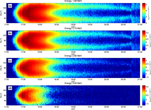
Figure 4. REPT-B pitch angle distributions on 2014 September 12 from 17:00 to 21:00 UT at 1.80–3.40 MeV energy channels. Before the magnetopause compression (∼17:30 UT), all energy levels presented 90°-peaked PAD shapes. Afterward, as the magnetopause compression progressed, the PAD shapes gradually changed to butterfly-like shapes, which are evidenced here by a local minimum flux at a 90° pitch angle.
Download figure:
Standard image High-resolution imageWe then used the electron fluxes in the 90° pitch angle bin from both the MagEIS-B and REPT-B instruments (Figures 5 and 6, respectively) to identify periods when the maximum flux intensity prior to the dropout decreased by 80% (roughly 1/e2). In what follows, we describe how we determined the times when the maximum flux at 90° decreased by 80%. Panels (a)–(d), (i)–(l), and (q)–(t) in Figure 5 show electron fluxes at 90° pitch angles. The blue circles are the pitch angle–resolved differential electron fluxes from MagEIS at different energy levels (from 169.3 to 1704 keV). A black line was overplotted on each of these panels, and each black line corresponds to the fitted curve obtained by the 3-Gaussian function shown in Equation (2) below:

where ai, ti, and ci are the fit parameters, and subscript i indicates the number of peaks to fit. There are two distinct time instants denoted by T1 and T2. The former corresponds to the time when the fitted flux achieved a global maximum within the analyzed interval, and the latter to the time when this maximum fitted flux decreased 80% (roughly 1/e2). We investigated the PAD shapes at each of these time instants, and they are shown in panels (e)–(h), (m)–(p), and (u)–(x) in Figure 5. The red and green lines correspond to the PAD shapes at time instants T1 and T2, respectively. Figure 7 presents the times T2 when electron fluxes at 90° pitch angles drop by 80% as a function of energy. The electron flux dropout at a 90° pitch angle occurs first for higher-energy electrons, as also shown in Figures 5(e)–(r) and 6. We point out that only electrons at energies equal to or above ∼160 keV exhibit an expressive decrease in the electron flux, while at lower energies a sustenance in the measured fluxes was detected, particularly at 90° pitch angles (Figures 5(a)–(d)).

Figure 5. Comparison between pitch angle–resolved electron fluxes before (T1) and during (T2) the electron flux dropout on 2014 September 12. Panels (a)–(d), (i)–(l), and (q)–(t) present a 90-minute interval (17:30–19:00 UT) of MagEIS-B electron fluxes (blue circles) at a 90° pitch angle for several energy channels ranging from 169.3 to 1704.0 keV. A Gaussian-like fit (see text for details) was also superposed (black curve) onto these plots. The time T1 corresponds to the maximum fitted flux value, whereas T2 corresponds to when the flux drops to 80% (roughly 1/e2) of this maximum value. The corresponding electron pitch angle distributions (PADs) at these two time instants are shown as red and green curves, respectively, in panels (e)–(h), (m)–(p), and (u)–(x). At T1 (T2), the electron PADs have a 90°-peaked (butterfly) shape, as evidenced by the r parameter, which provides the ratio between the flux at the 90° pitch angle bin to the average flux at both 40.9° and 139.1° pitch angle bins. It is defined that whenever r > 1.1 (r < 0.9), the analyzed electron PAD has a 90°-peaked-like (butterfly-like) shape (see text for details).
Download figure:
Standard image High-resolution image
Figure 6. Comparison between pitch angle–resolved electron fluxes before (T1) and during (T2) the electron flux dropout on 2014 September 12. Panels (a)–(d) present a 2 hr interval (17:00–19:00 UT) of REPT's B electron fluxes (blue circles) at a 90° pitch angle for several energy channels ranging from ∼1.80 MeV to ∼3.4 MeV. A Gaussian-like fit (see text for details) was also superposed (black curve) onto these plots. The time T1 corresponds to the maximum fitted flux value, whereas T2 corresponds to when the flux drops to 80% (roughly 1/e2) of this maximum value. The corresponding electron pitch angle distributions (PADs) at these two time instants are shown as red and green curves, respectively, in panels (e)–(h). At T1 (T2), the electron PADs have a 90°-peaked (butterfly) shape, as evidenced by the r parameter, which provides the ratio between the flux at the 90° pitch angle bin to the average flux at both 47.6° and 132.4° pitch angle bins. It is defined that whenever r > 1.1 (r < 0.9), the analyzed electron PAD has a 90°-peaked-like (butterfly-like) shape (see text for details).
Download figure:
Standard image High-resolution image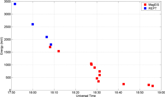
Figure 7. Time instant where the pitch angle–resolved electron flux drops significantly (about 80% of the maximum value) for energy channels ranging from ∼200 keV to ∼2250 keV by MagEIS (red squares) and from ∼1.8 MeV to ∼3.4 MeV by REPT (blue squares).
Download figure:
Standard image High-resolution image3.3. Investigating Electron Drift Paths Using a Magnetic Field Model
Radiation belt particles with different energy levels could be lost to the magnetosheath since the magnetopause reached around L ∼ 7, as far as our MHD simulation is concerned (for more details, see the outputs of the simulation under the run number Vitor_Souza_062816_1 at the CCMC website). For lower-energy (up to 160 keV) electrons, even if they were lost to the magnetosheath during storm conditions, they could be resupplied by injections in the nightside region, which could explain the electron flux increase at lower energy levels. A deeper analysis about such a flux increase during this event is out of the scope of this study. At higher energies, however, the flux dropout at 90° developed and persisted for the remainder of the period shown (Figures 3(e)–(r) and 4). This indicates that equatorially mirroring particles may have been lost from the distribution, and there was no considerable enhancement to repopulate the radiation belt during the interval of interest. The drift path for equatorially mirroring particles, considering the conservation of the first and second adiabatic invariants, can be determined using the following equation (Min et al. 2013; Kang et al. 2016):
where  is the Lorentz factor, v is the electron velocity, e is the electron charge, me is the electron rest mass, c is the speed of light, μ is the first adiabatic invariant (magnetic moment), Bm is mirror point magnetic field strengths at given second adiabatic invariant, and
  is the electric convection (corotation) potentials (see e.g., Min et al. 2013; Kang et al. 2016, and references therein). For relativistic (≳1 MeV) electrons, Equation (3) becomes
  , which means that the field-line curvature and grad B drifts dominate over the E × B drift (Kang et al. 2016). However, for electrons with lower energies (≤100 keV), the E × B drift is dominant (see Appendix).
To investigate electron drift paths in different pitch angles, we used the empirical TS04 magnetic field model (Tsyganenko & Sitnov 2005) and the W2k electric field model (Weimer 2001). Figures 8(a1)–(a4) show isocontours of convective potential (in units of kV) calculated using the W2k model. The electron drift shells were calculated through Equation (3) at fixed first μ and second K adiabatic invariants, as shown in Figure 8. The values of μ and K were chosen in such a way to correspond to ∼1 MeV energy electrons, with equatorial pitch angles αeq ∼ 86° (Figures 8(b1)–(b4)) and αeq ∼ 23° (Figures 8(c1)–(c4)) at L = 5, i.e., μ = 789 MeV/G and  , μ = 121 MeV/G and
  , respectively. The Sun is on the right, and the rightmost curve indicates the magnetopause in each plot. Because convective potentials are well below 1 MeV, the drift paths of electrons with ∼1 MeV energies are nearly independent from the convective potential contours. The electron drift paths passing L = 4, 5, and 6 at MLT = 2 (blue lines in Figure 8) were totally closed at 16:00 UT, and after 15 minutes, the drift paths at L ≥ 6 were intersected by the magnetopause, as presented in Figures 8(b2)–(b4).

Figure 8. The convective potential and the electron drift paths calculated using the W2k model during 2014 September 12, in an equatorial plane, for L-shell 2–7. The three reds stars represent the L-shell positions 4, 5, and 6 at MLT = 2. The upper panels show isocontours of convective potential (kV) at (a1) 16:00 UT, (a2) 16:15 UT, (a3) 16:50 UT, and (a4) 18:00 UT. Drift paths at αeq ∼ 86° at (b1) 16:00 UT, (b2) 16:15 UT, (b3) 16:50 UT, and (b4) 18:00 UT for μ = 789 MeV/G and k = 0.00091  at L = 5. The αeq ∼ 23° at (c1) 16:00 UT, (c2) 16:15 UT, (c3) 16:50 UT, and (c4) 18:00 UT for μ = 121 MeV/G and k = 0.72
  at L = 5 (see text for details).
Download figure:
Standard image High-resolution imageThis result matches those found in our global MHD simulations, wherein the outermost magnetic field strength isocontour was reached by the magnetopause boundary after the magnetospheric compression caused by the ICME arrival (see Figure 2(f)). Note that the drift paths for electrons at L ≤ 7 for αeq ∼ 23° were kept closed (Figures 8(c1)–(c4)). The αeq ∼ 86° electron drift paths were reached by the magnetopause, at L ≥ 5, only after 17:00 UT (Figure 8(b3)). The open drift paths persist at L > 5 until 18:00 UT (Figure 8(d)), which suggests electrons with energy of ∼1 MeV at L > 5 could have been lost to the magnetosheath until 18:00 UT. During the interval, the αeq ∼ 23° electron drift paths were not intersected by the magnetopause and were kept closed, which provides an explanation for the observed trapped electrons at αeq ∼ 23° and αeq ∼ 157° seen even after the dropout. The first evidence of PAD dropout in Figure 4 was observed only after 17:48 UT. Such divergence in the dropout time onset can be explained in the following way: The satellite position was not favorable to measure particles at L ≥ 4.5 before 17:48 UT, i.e., the satellite was moving toward the apogee of its orbit. If the spacecraft was in the apogee before 17:48 UT, it would have most likely observed the dropout.
4. Investigating the Effects of EMIC Waves on 2014 September 12
Jaynes et al. (2015), Alves et al. (2016), and Ozeke et al. (2017) discussed the contribution of magnetopause shadowing, ULF waves, and coherent chorus waves to the electron flux dropout observed on 2014 September 12. However, the mechanism studied by these authors did not include the contribution from relativistic electron scattering to the atmosphere due to EMIC waves.
Theoretical, modeling, and observational studies have considered pitch angle scattering by EMIC waves as the dominant mechanism to scatter relativistic electrons to the atmosphere (Thorne & Kennel 1971; Lyons & Thorne 1972). EMIC waves are associated with ion cyclotron instabilities, which are usually excited by ring current ion injections during magnetic storms, and also during magnetopause compressions (Thorne et al. 2013). In this context, EMIC waves appear mostly left-hand polarized, in the Pc1-2 ULF frequency range (0.1–5 Hz), and the wave amplitude varies from 0.1 to tens of nT (Halford et al. 2016). The major ion components of the radiation belt are  , He +, and
  , which suggests that waves that approach the gyrofrequency of these ions are responsible for the gyroresonance interaction with the relativistic electrons. EMIC waves are usually confined between ion gyrofrequency bands, because of the wave propagation stopband frequencies. The EMIC wave resonant interactions with relativistic electrons above 1 MeV are possible and are strongly associated with the plasma composition (Summers & Thorne 2003). The plasma composition controls the cutoff frequency and the preferential band where the waves are excited. After these interactions, one of the most important effects is that relativistic and ultra-relativistic electrons can rapidly (within an hour) be scattered into the atmosphere, causing dropouts in the outer radiation belt electron fluxes (Summers & Thorne 2003).
For the dropout event being analyzed here, in order to explore the EMIC waves occurrence, the power spectral density (PSD) was calculated based on the magnetic field perturbation  , where Bavg is a 100 sec time average of the B field, as done by Wang et al. (2015). We performed a Short-Time Fourier Transform with a window length of 3750 samples (∼1 minute), and an overlap of 1875 samples (∼30 s). The EMIC-wave frequency range (0.1–2 Hz) is shown in Figures 9 and 10 for RBSP-A (RBSP-B) measurements along the three orbits on 2014 September 12. The panels show (a) the power spectral density, (b) the PAD, (c) MLT, and (d) the L-shell parameter.
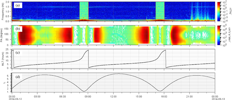
Figure 9. (a) Magnetic field magnitude's power spectral density (PSD), (b) pitch angle distribution at 2.10 MeV energy channel, (c) MLT, and (d) L-shell parameter obtained by Van Allen Probe A on 2014 September 12. We note that the PSD signal at around 1.5 Hz corresponds to the satellite spin tone.
Download figure:
Standard image High-resolution image
Figure 10. (a) Magnetic field magnitude's power spectral density, (b) pitch angle distribution at 2.10 MeV energy channel, (c) MLT, and (d) L-shell parameter obtained by Van Allen Probe B on 2014 September 12.
Download figure:
Standard image High-resolution imageAt the time when EMIC waves were observed at the RBSP-B location, we did not see EMIC waves at the RBSP-A position. It seems to be that the EMIC wave activity did not cover a large area to reach both spacecraft positions. On the other hand, the EMIC wave activity was not long enough to be observed by both spacecraft even when, one hour later, the RBSP-A crossed the same MLT region (see Figures 9(c) and (d)). The magnetic PSD from both RBSP showed broadband, impulsive vertical streaks that will not be treated here.
The dawnside sector is a slightly less favorable local time region for EMIC waves occurrence (see e.g., Saikin et al. 2015, and references therein). Still, the importance of the local in situ observations were relevant because EMIC waves are a very localized and sporadic phenomena (Zhang et al. 2016b). The Van Allen Probes mission provides us with an unique opportunity to disentangle spatial from temporal features in the observations.
All measured magnetic field components, i.e., parallel, azimuthal, and radial, showed similar signatures of EMIC waves with essentially equal power in all three components (not shown). EMIC waves are generally transverse, with little or no compressional component, thus such observations are somewhat unusual. The impact of this unusual nature is not clear, so further investigation on this matter might be worthwhile, but we will not treat this issue here. The parallel ( ) component was chosen as an example of the EMIC wave occurrence on 2014 September 12 after 19:00 UT. The time resolution used here was 1/64 s (64 Hz). The results were plotted in Figure 11(a), and the
  , He+, and
  gyrofrequencies were overplotted. During the interval analyzed in this study, Hydrogen band (H+) EMIC waves have been observed. Figures 11(c)–(e) present successive zoom-ins of a given EMIC wave packet. The Y-axis shows the magnetic field perturbation (
 ), and from it we estimated the peak wave amplitude (∼2 nT) and the frequency varies from ∼0.5 up to 1 Hz. The minimum resonance energy was calculated following Equation (4) (see e.g., Summers & Thorne 2003; Kang et al. 2016, and references therein):

where
 is the electron velocity parallel to the field line, me is the electron rest mass, ω and k are the angular frequency and wave number of EMIC waves, respectively, Ωe is the electron gyrofrequency, n is the resonance harmonic number (assumed to be 1), and finally s is set to be −1 for the left-hand mode. The minimum resonant energy is strongly dependent on the plasma composition, the wave frequency, and the background magnetic field B0 (see e.g., Summers & Thorne 2003; Kang et al. 2016, for more details). We assumed
  ,
,  , and
, and  (Summers & Thorne 2003). We used cold plasma dispersion and assumed to be
  and the electron number density was given by the spacecraft potential. The minimum resonance energy was 1.2 MeV, which strengthens the claim that the EMIC wave packets observed in this event can resonantly interact with ≥1.2 MeV electrons and scatter them into the atmosphere.
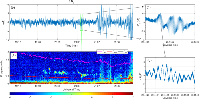
Figure 11. Occurrence of EMIC waves observed by Van Allen Probe B. (a) Wave power spectrogram in the range of 0.1–2 Hz for the 18:00 to 23:00 UT period on 2014 September 12. The magenta, red, and black lines correspond to ion gyrofrequencies for hydrogen, helium, and oxygen, respectively. (b) Time series of the variation (relative to a 100 s local average of the background) parallel magnetic field component in the MFA coordinate system. The most intense oscillations in the magnetic field correspond to EMIC waves. (c) Detailing of an intensified magnetic field variation during the analyzed event shows EMIC wave packets. (d) An interval of 22 s of data showing a wave packet in detail. The central frequency is about 0.6 Hz, and the maximum amplitude of the disturbance is approximately 2 nT.
Download figure:
Standard image High-resolution image5. The Reconfiguration of the PAD Shape
The electron PADs obtained by both MagEIS-B and REPT-B instruments showed evidence of electron losses over a wide range of energy levels, as described below. Before the magnetopause compression, the PADs were primarily 90°-peaked for all energy channels (Figures3 and 4). Afterward, for energies >132 keV, the dropout caused by magnetopause shadowing changed these PAD shapes into butterfly-like shapes, as shown in Figures 3(f)–(r) and 12(a) and (c). Energy levels ≤132 keV did not respond in the same way, i.e., the 90°-peaked PAD shape was sustained throughout the analyzed (∼3 hr) period (Figures 3(a)–(e)).
The energy channels between 132 keV and 1.0 MeV, measured by MagEIS-B, showed the dropout in pitch angles near 90° (Figure 12(a)) and belatedly, at 20:31 UT, their PAD shapes remained as butterflies, similar to the one at 19:40 UT (the dotted line in Figure 12(b)). However, at energies above 1 MeV (Figure 12(c)), as measured by both MagEIS-B and REPT-B, a new PAD shape feature emerged. The two characteristic peaks in the electron flux of the butterfly PADs were close to 30° and 150° at 19:40 UT (the black line in Figure 12(d)). Afterward, the two peaks moved to ∼45° and ∼135°, resulting in a different butterfly PAD (the dotted line in Figure 12(d)). Such a pitch angle transition of the two peak fluxes suggests that some physical mechanism favored precipitation into the loss cone. Previous studies showed the butterfly PAD in this region as a result of drift-shell splitting (Sibeck et al. 1987). Figure 10(a) showed that, in fact, the butterfly PAD shape is recurrent on L-shells larger than 5. In addition, when gyroresonant interactions mediated by EMIC waves were present, the persistent decrease in electron flux near the loss cone was evident. We then suggest that such interactions were the main contributors for generating the peculiar butterfly PAD shape, since EMIC waves were detected by EMFISIS-B during the aforementioned PAD shape reconfiguration, and they are known to effectively pitch angle scatter relativistic electrons (Summers et al. 2007; Shprits et al. 2009; Li et al. 2014; Usanova et al. 2014; Zhang et al. 2016a; Clilverd et al. 2017).

Figure 12. Comparison of electrons PAD at different energy levels from the REPT and MagEIS instrument on board Van Allen Probe B on 2014 September 12 from 17:00 to 21:00 UT. (a) Normalized PAD electron flux at the 466.8 keV energy level. (b) Sequences of PAD during the interval selected in the black box above (19:40–20:31 UT) representing the beginning of EMIC waves. (c) Normalized PAD electron flux at the 1.80 MeV energy level. Butterfly PAD at (d) 1.80 MeV energy channel. The solid line represents the instant before EMIC waves, and the dotted line during EMIC waves shown in (c) as black arrows.
Download figure:
Standard image High-resolution imageFigure 13 summarizes some physical mechanisms involved in the generation of the PAD shape reported in this work. The initial dropout of relativistic electron fluxes resulted from magnetopause shadowing. The relativistic electrons with equatorial pitch angles near the loss cone remained, in part, trapped until the occurrence of EMIC waves at around 19:30 UT. After this time, scattering into the atmosphere was intensified by gyroresonant interactions with EMIC waves, resulting in the unusual PAD.
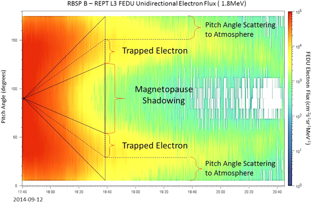
Figure 13. Pitch angle omnidirectional electron flux spectrogram in 1.8 MeV energy channel during 2014 September 12 between 17:40 and 21:00 UT. The electron flux dropout observed after 18:30 UT in pitch angles close to 90° seems to be due to magnetopause shadowing. The dropout in pitch angles lower than 30° and higher than 150° after 19:00 UT corresponds to pitch angle scatter into atmosphere.
Download figure:
Standard image High-resolution image6. Concluding Remarks
On 2014 September 12, the Earth's magnetosphere was impinged by an ICME. The twin Van Allen Probes measured an electron flux dropout at several energy levels. Previous studies attributed the major cause of this dropout to magnetopause shadowing followed by enhanced ULF wave activity, as well as a gyroresonant interaction with coherent whistler mode chorus waves. However, the presence and role of EMIC waves were not confirmed until this work.
We used the global MHD SWMF/BATS-R-US model coupled with the RCM module to self-consistently model the Earth's magnetospheric field for the period encompassing the ICME arrival at Earth. The MHD simulation showed that the ICME-related compression "opened" the previously closed and outermost electron drift paths, i.e., the magnetic field strength isocontours. These paths most likely led to the Van Allen Probes location, and the corresponding drifting relativistic electrons intercepted the magnetopause, thus escaping to the magnetosheath region. The empirical TS04 magnetic field model (Tsyganenko & Sitnov 2005) and W2k electric field model also showed the higher-energy (up to 2 MeV) electron's drift paths at L-shells commensurate to those at Van Allen Probes could indeed reach the magnetopause, thus confirming the likelihood of the magnetopause shadowing scenario. The dropout was first seen in electron PADs at higher (>1 MeV) energies. Losses due to magnetopause shadowing or drift-shell splitting were observed as a decrease in flux at pitch angles near 90°. This event showed an electron flux dropout for electron energies above 132 keV, with the loss of higher-energy electrons being observed before the lower-energy ones. The observed PADs had butterfly shapes with two peaks around 30° and 150° after the magnetopause compression, while electrons at energy levels ≤132 keV exhibit a 90°-peaked or pancake PAD shape throughout the analyzed period.
Further PAD analysis showed an unusual PAD for electrons only at relativistic energies. The two peaks in the butterfly PAD, which had previously been around 30° and 150° pitch angles, moved to ∼45° and ∼135°, resulting in a peculiar butterfly-like PAD shape. Decreases in the relativistic electron flux at pitch angles near the loss cone matched the times when EMIC waves were measured by the EMFISIS instrument on board the RBSP-B satellite. We emphasize that the EMIC waves were transient and/or localized, and only RBSP-B observed them in this event. Following RBSP-B by 60 minutes, RBSP-A detected no waves at this moment in the Pc1-2 frequency range. Despite the fact that the RBSP-B orbit was in the dawnside sector, where the occurrence of EMIC waves is somewhat less common, we believe that the unusual electron PAD at relativistic energies and several EMIC wave packets observed in the magnetic field power spectral density over the analyzed period provide strong evidence for relativistic electron losses due to EMIC waves. Investigations regarding the appearance of such unusual PADs in RBSP data will be addressed in a future work.
Processing and analysis of both the MagEIS and REPT data were supported by the Energetic Particle, Composition, and Thermal Plasma (RBSP-ECT) investigation funded under NASA's Prime contract no. NAS5-01072. All RBSP-ECT data are publicly available at the website http://www.RBSP-ect.lanl.gov/. Solar wind parameters were measured by the ACE satellite, and they are available at the website http://www.srl.caltech.edu/ACE/ASC/level2/. This work was carried out using the SWMF/BATS-R-US tools developed at the University of Michigan Center for Space Environment Modeling (CSEM) and made available through the NASA Community Coordinated Modeling Center (CCMC). V.M.S. thanks the São Paulo Research Foundation (FAPESP) grant 2014/21229-9. L.A.D. and P.R.J. are grateful for financial support from China Brazil Joint Laboratory for Space Weather. A.D., M.R., and O.M. thank the Brazilian National Council for Research and Development (CNPq) via the PCI grant 304209/2014-7, 308452/2018-6, 424352/2018-4 and 307083/2017-9, for the financial support. D.B. thanks NASA for support the Van Allen Probes program at LASP/CU. Work at NASA Goddard Space Flight Center was supported by the Van Allen Probes mission. The authors thank Remya Bhanu for helpful conversations. Development (CNPq) via the PCI grant 304209/2014-7, respectively, for the financial support. The authors thank Remya Bhanu for helpful conversations.
Appendix: Isocontours of Convective Potential in Different Electron Energies
Figures 14 (a1)–(a4) show isocontours of convective potential (kV) calculated using the W2k empirical electric field model (Weimer 2001). Panels (b1)–(c4) show electrons drift paths similar to those shown in Figure 8, but μ and K are chosen to correspond to ∼30 keV electrons. Panels (b1)–(b4) and (c1)–(c4) correspond to electron drift paths with αeq ∼ 86° and 23° at L = 5, respectively. The electron drift paths are very different from those for ∼1 MeV, as shown in Figure 8. First, drift paths at L ≥ 5 are similar to convective potential contours (a1)–(a4). This means that drift paths at L ≥ 5 are significantly influenced by convective potentials. At L ≤ 5, corotation electric field dominates convective electric field, and thus drift paths are quite circular. Second, drift paths with αeq ∼ 86° and 23° are not quite different. Thus, we may not be able to expect butterfly PADs. Third, drift paths at L ≥ 5 are connected by both plasma sheet regions on the nightside and the magnetopause on the dayside. This implies that electrons can be both injected on the nightside and lost on the dayside.

Figure 14. The convective potential and the electron drift paths calculated using the W2k model during 2014 September 12, in an equatorial plane, for L-shell 2–7. In this case, μ and K are chosen to correspond to ∼30 keV electrons.
Download figure:
Standard image High-resolution imageFigure 15 presents the same plots as shown in Figure 14, but μ and K are chosen to correspond to ∼100 keV electrons. Overall, electron drift paths in Figures 15(b1)–(c4) are very different from those for ∼30 keV (Appendix) or ∼1 MeV (Figure 8). At L ∼ 5, electron drift paths with αeq ∼ 86° in (b1)–(b4) are open, while those with αeq ∼ 23° are often closed. This suggests that butterfly PADs may happen.
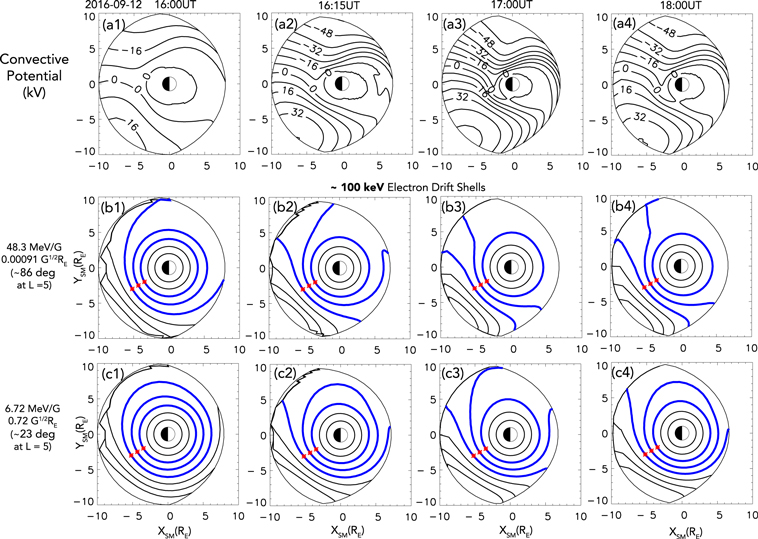
Figure 15. The convective potential and the electron drift paths calculated using the W2k model during 2014 September 12, in an equatorial plane, for L-shell 2–7. In this case, μ and K are chosen to correspond to ∼100 keV electrons.
Download figure:
Standard image High-resolution imageFigure 16 followed the same plots as shown in Figures 14 and 15, but μ and K are chosen to correspond to ∼500 keV electrons. Electron drift paths in Figures 16(b1)–(c4) are very similar to those shown in Figure 8. The same configuration were observed in Figures 17(b1)–(c4), when μ and K are chosen to correspond to ∼2 MeV electrons.
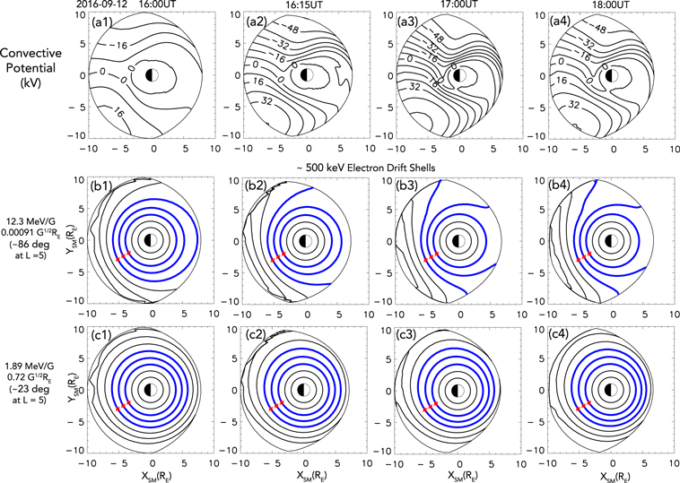
Figure 16. The convective potential and the electron drift paths calculated using the W2k model during 2014 September 12, in an equatorial plane, for L-shell 2–7. In this case, μ and K are chosen to correspond to ∼500 keV electrons.
Download figure:
Standard image High-resolution image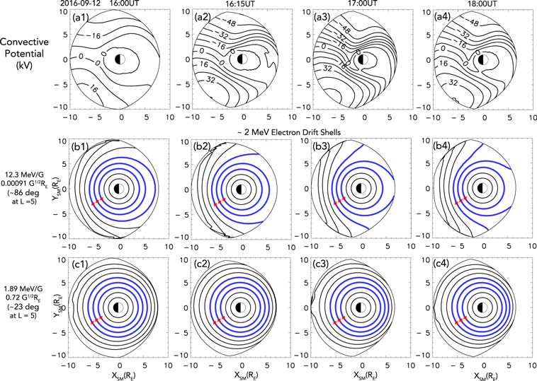
Figure 17. The convective potential and the electron drift paths calculated using the W2k model during 2014 September 12, in an equatorial plane, for L-shell 2–7. In this case, μ and K are chosen to correspond to ∼2 MeV electrons.
Download figure:
Standard image High-resolution image
Thus, the results suggest that in both cases (∼500 keV and ∼2 MeV electrons), butterfly PADs may happen as described in Section 3.1.
Footnotes
- *
Released on 2018 October 8.