


Abstract
We present a study of the origin of one interplanetary coronal mass ejection (ICME) that lacked an easily identifiable signature of an associated progenitor coronal mass ejection (CME) near the Sun in the observations of SOHO/LASCO at the L1 point. We consider these kinds of ICMEs as problematic, as they pose the difficulty of understanding the Sun–Earth connection and providing space weather warnings; understanding the causes of problematic ICMEs is important for space weather forecasting. This study presents the first detailed analysis of a geoeffective problematic ICME that occurred on 2011 May 28, whose progenitor CMEs are difficult to identify in LASCO images, but fortunately they were captured by SECCHI on board the STEREO spacecraft in the quadrature configuration. There are two progenitor CMEs launching from the Sun in succession of 8 hours. We apply the graduated cylindrical shell model to reconstruct the 3D geometry, propagating direction, velocity, and brightness of the two CMEs. The main cause of the first CME (CME-1) invisible in SOHO/LASCO is due to its low mass; that is, when the CME emerges above the occulter, its brightness is as faint as the noise. The second CME (CME-2) is small, including a narrow angular width and a small cross-section of the magnetic flux rope. Even though propagating toward the Earth, CME-2 appeared as a narrow CME instead of as a halo or partial halo CME in the LASCO field of view. We also show that CME-2 propagates faster than CME-1, and that they might have interacted in the interplanetary space.
Export citation and abstract BibTeX RIS
1. Introduction
An Earth-affecting interplanetary coronal mass ejection (ICME) is generally considered to be the counterpart of an Earth-directed coronal mass ejection (CME) that originated from the Sun. An Earth-directed CME, or a CME propagating along the Sun–Earth line, usually appears as a full halo (360°) or partial halo (>120°) surrounding the occulter of observing coronagraphs located near Earth (Howard et al. 1982b). Halo CMEs have been well observed and studied since the advent of the Large Angle and Spectrometric Coronagraph (LASCO) suite (Brueckner et al. 1995) on board the SOlar and Heliospheric Observatory (SOHO) situated at the L1 point since 1996 January. However, it is also known that ICMEs identified by in situ observations do not show a one-to-one correspondence with front-side halo CMEs (Webb et al. 2000b; Wang et al. 2002; Zhao & Webb 2003; Yermolaev et al. 2005; Shen et al. 2014). Yermolaev & Yermolaev (2006) found that about 18%–44% ICMEs are not preceded by an identifiable front-side halo CME in the LASCO coronagraph. The lack of an identifiable front-side halo CME poses a great challenge to space weather forecasting ability. Those ICMEs have been regarded as problematic storms because they do not allow the identification of the progenitor CMEs for geomagnetic storms, including intense ones occurring at Earth (Webb et al. 1998; Zhang et al. 2003; Schwenn et al. 2005). Following Webb et al. (1998) and Zhang et al. (2003), we call these kinds of ICMEs problematic ICMEs, which are unambiguously identified by in situ observations near Earth, but which lack apparent association with any identifiable progenitor CME near the Sun, as observed by existing coronagraphs located along the Sun–Earth line, such as SOHO/LASCO. This is different from the usage of a "stealth" CME, which refers to an observed CME near the Sun in the coronagraph images, but without identifiable eruptive signatures on the solar disk (Robbrecht et al. 2009; Ma et al. 2010; Wang et al. 2011; Howard & Harrison 2013; Nitta & Mulligan 2017; Hess & Zhang 2017). In this study, we intend to address the causes of problematic ICMEs, as they pose a significant challenge to any effective space weather prediction.
One could think of two possible limitations of detecting Earth-directed CMEs along the Sun–Earth line. The first is the projection effect. The occulting disk of a coronagraph is necessarily needed to block the intense emission light from the solar disk. A CME can only be visible when the projected size of the CME exceeds the diameter of a coronagraph's occulting disk (Webb et al. 1998). An Earth-directed CME, approximated by a cone-like geometry, would have a smaller projected size than a CME propagating away from the Sun–Earth line. The second limitation is the Thomson scattering effect (Minnaert 1930), e.g., according to the plane-of-the-sky assumption (Vourlidas & Howard 2006), in the coronagraph observations; the plane of the maximum scattering coincides with the plane of the sky. Thus, both the projection and Thomson scattering effects indicate that limb CMEs suffer the least, and are supposed to be most visible. Webb & Howard (1994) found that the coronagraphs detected significantly fewer CMEs that originated with 45° of the Sun center, which further established the CME visibility function for coronagraphs. Yashiro et al. (2005) studied the visibility function of LASCO observations. Howard et al. (1982a), Michels et al. (1997), and Vourlidas & Howard (2006) also found that limb CMEs are brighter and more easily detected by coronagraphs located near the Earth than those originating near the disk center.
Hence, to find the corresponding Earth-directed CMEs, an effective way is to use the coronagraph observations from satellites off the Sun–Earth line, such as the Solar TErrestrial RElations Observatory (STEREO; Kaiser et al. 2008) mission launched in 2006. STEREO included two satellites, one leading (STEREO A: STA) and one trailing (STEREO B: STB) the Earth. Both satellites are slowly separating from the Earth at a rate of 22 5 per year. The Sun–Earth Connection Coronal and Heliospheric Investigation (SECCHI; Howard et al. 2008) suite on board STEREO provides simultaneous Thomson scattered white-light observations of CMEs from two different view angles. Combined with the observations from SOHO/LASCO at L1 point, true 3D structures of CMEs can now be reconstructed, and these structures can be continuously tracked from low coronal to 1 au or even beyond. Thernisien et al. (2006) has developed a graduated cylindrical shell (GCS) model for reconstructing the 3D geometry, propagation direction, and simulating brightness structure of CMEs.
ICMEs can be recognized by in situ solar wind observations based on certain well-known criteria, including enhanced magnetic field strength, smoothly changing magnetic field direction, abnormal low proton temperature, low proton plasma β, etc. (Burlaga et al. 2001; Cane & Richardson 2003; Jian et al. 2006, 2008; Chi et al. 2016). ICMEs are the main source of geomagnetic storms, especially for intense geomagnetic storms (Zhang et al. 2003; Xue et al. 2005; Gopalswamy 2006; Yermolaev & Yermolaev 2006; Zhang et al. 2007; Wu & Lepping 2008). A CME observed as full halo or partial halo from the near Earth coronagraphs is an excellent indicator of possible geoeffectiveness (Brueckner et al. 1995; Webb et al. 1998; Kim et al. 2008). However, the existence of problematic ICMEs complicates the task of space weather forecasting. A direct consequence is that there would be a significant fraction of geomagnetic storms, which could not be predicted. In in situ observations, geoeffective ICMEs are usually of large-scale magnetic flux ropes having average diameter about 0.2 au (e.g., Zhang et al. 2008; Wang et al. 2015). There also exist small-scale flux ropes with diameters less than 0.1 au (Moldwin et al. 2000). Rouillard et al. (2011) first established the link between narrow CMEs and small in situ flux ropes.
In this paper, we will answer the question of why there exist problematic ICMEs by using the best available observations of CMEs from multiple viewing angles in space and by continuous tracking from the Sun to Earth. We will make a detailed and comprehensive analysis of a geoeffective ICME associated with two weak, narrow, Earth-directed CMEs only revealed from observation of STEREO. Further, this study will also help address the issue of the sources of small-scale magnetic clouds, whose diameters are less than 0.1 au near Earth (Feng et al. 2007). The sources of small-scale flux ropes remain elusive.
The paper is organized as follows. In Section 2, we present in situ observations of the problematic ICME. In Section 3, we provide observations from STEREO SECCHI and analyze the causes of problematic ICME. We revisit the in situ observations and argue that the problematic ICME contains two consecutive magnetic flux ropes in Section 4. A summary of our main results and a discussion are presented in Section 5.
2. In situ Observations of the Problematic ICME
The problematic ICME studied in this paper occurred on 2011 May 28. As observed by the WIND spacecraft near Earth, the ejecta part of the ICME arrived at ∼05:30 UT on 2011 May 28, and lasted for almost 16 hr until ∼21:00 UT on May 28. The in situ properties of this ICME are shown in Figure 1. The gray area in Figure 1 indicates the region of the ejecta part of the ICME, which is characterized by a weakly enhanced magnetic field, a smoothly changing magnetic field direction, a lower proton temperature than expected (Richardson & Cane 1995), and an abrupt reduction of plasma β parameter. No apparent shock or jump of plasma parameters was detected by the in situ observation prior to the arrival of the ejecta. There is no doubt that the observed properties of the event match the ICME identification criteria as discussed in Wu & Lepping (2011), Shen et al. (2014), Chi et al. (2016 and references therein). This ICME is not only on our ICME list (http://space.ustc.edu.cn/dreams/wind_icmes/), but also on Richardson and Cane's ICME list (Richardson & Cane 2010, start time: 2011 May 28 05:00, end time: 2011 May 25 21:00) and in the Lepping MC list (Lepping et al. 2015, start time: 2011 May 28 06:06, end time: 2011 May 28 16:06).
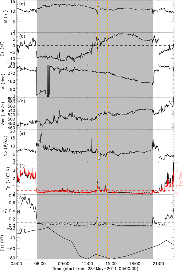
Figure 1. Observations of solar wind magnetic and plasma properties by WIND spacecraft during 3:00–23:00 UT on 2011 May 28. From top to bottom, panels are magnetic field strength (B), z-component of the magnetic field in GSM coordinate system (Bz), azimuthal (ϕ) angles of the field direction in GSM coordinate system, solar wind speed (V), proton density (Np), proton temperature (Tp), the ratio of proton thermal pressure to magnetic pressure (β), and the Dst indices from WDC. The gray shaded region shows the ejecta part of ICME. The orange vertical dashed line shows a discontinued region of this ICME.
Download figure:
Standard image High-resolution imageAs shown in panel (a), the total magnetic field strength of the event shows a profile of smooth rotation and low variability with an average value of 11.5 nT. Panel (b) shows that the ICME initially carried a strong southward magnetic field lasting for almost 7 hr until around 12:40 UT, with a negative peak value of −12.8 nT. This 7 hr long duration of southward magnetic field triggered a moderate geomagnetic storm, reaching the minimum value of Dst of −80 nT at 12:00 UT and 15:00 UT. After 12:40 UT, the direction of the z-component of the magnetic field started to turn northward, and the Dst index started to recover. Panel (c) presents the azimuthal (ϕ) angles of the magnetic field direction, which also clearly show the rotation of the magnetic field. The velocity within the ICME ejecta shows a gradual increasing profile (panel (d)), possibly in response to the squeezing of a corotating interaction region following the ICME. The ICME average speed is 517 km s−1, corresponding to a travel time of about 80h from the Sun to its arrival at Earth. In the middle of the ICME event, there exists an interesting short-interval structure of about one-and-a-half hour marked by the two orange vertical lines. During this short interval, the total magnetic field and the z-component of the magnetic field have two small bumps. The magnetic field direction does not show a clear sign of rotation. The temperature of proton and proton plasma β also show an instantaneous increase at the beginning and end of the interval, which are very like the interaction region between two successive magnetic clouds as shown in Wang et al. (2003) and Mishra et al. (2015). This kind of peculiar behavior within an apparent ICME event could not be understood until we carefully examined CME observations from STEREO. Our analysis helps to understand that the identified in situ structure contains two independent ICME ejecta, but are closely connected in time and space. Details of the relation of the two ejecta will be presented in the following sections.
3. Remote-sensing Observations and Analysis of the Problematic ICME
According to the ICME average speed in situ, the progenitor solar CME should have erupted about 80 hr earlier prior to the ICME's arrival. As the projected speed of halo CME is quite slow, we prefer to use base-difference images with large time differences to search for the progenitor CME in a conservative 120 hr long continuous window of SOHO/LASCO observations. We also check the CDAW LASCO CME catalog (Yashiro et al. 2004), which listed the CME's first appearance date and time, central PA, PA width in SOHO/LASCO. On the basis of the observations and CME catalog, during the research window, only one partial halo CME was detected by SOHO/LASCO. However, this partial halo CME can be confirmed as a backside eruption relative to the Earth, according to STEREO COR2 observations. So in the search window, there were only several narrow CMEs based on their projected shape in the field of view (FOV) of SOHO/LASCO. Using SOHO observations alone; we could not associate any one of these narrow CMEs as the progenitor of the observed ICME. Hence, based on the definition discussed above, the ICME is regarded as a problematic ICME.
The solar source of the ICME has to be sought using observations of spacecraft off the Sun–Earth line other than SOHO. On the days of the event, STA and STB are in the quadrature configuration, separated by approximately 90◦ from Earth: 935 west, 936 east, respectively. In such a quadrature configuration, an Earth-directed CME is viewed as a limb CME, which can be much more easily detected by the instruments and identified by observers, in the FOV of STA and STB COR2/HI1. This provides an unprecedented opportunity to track the problematic ICME backward from the in situ observations to the progenitor CME from side views. By following the problematic ICME back to the coronal, two candidate progenitor CMEs were detected by COR2 and HI1 in STA and STB, on 2011 May 25. The two Earth-directed CMEs were well observed through the entire SECCHI FOV. The first CME (hereafter CME-1) appeared in the FOV of STA and STB COR2 at 05:39 UT on May 25, while the other one (hereafter CME-2) first emerged at 13:39 UT, with a temporal separation of ∼8 hr between the two CMEs. We note again that no visible front-side halo CME was detected in the FOV of LASCO C2/C3. The challenging question is why is there no clear signatures of visible halo CME in LASCO observations for this Earth-affecting ICME? To answer this, we analyze the two candidate CMEs through the full usage of observations from COR2, HI1 of both STA and STB and C2/C3 observations from SOHO/LASCO.
3.1. The Observation and Analysis of CME-1 on 2011 MAY 25
Based on the first appearance time of CMEs in the coronagraphs, we further searched for the potential solar sources of these CMEs using the observations from the Advanced Imaging Assembly (AIA; Lemen et al. 2011) on board the Solar Dynamic Observatory (SDO). We find that CME-1 is associated with a weak, low coronal activity occurring at S16° W13°. The only apparent signal on the solar disk indicating a possible eruption is a small-scale post-eruption arcade (PEA) associated with a weak B1.9 class GOES X-ray flare. Figure 2 panel (a) shows the PEA of CME-1 in SDO AIA 211  band. The green line shows the tilt angle (−73°) of the PEA axis, which is defined as the clockwise rotation angle with respect to the east direction.
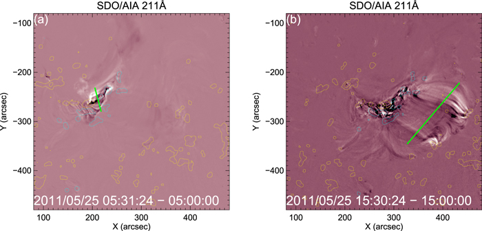
Figure 2. Images from SDO AIA 211  band superimposed by the contours of the SDO/HMI line of sight magnetogram. Panels (a) and (b) show the the post-eruption arcades associated with CME-1 and CME-2, respectively. The yellow and blue contours in each panel show the positive and negative magnetic field. The green line indicates the orientation of the post-eruption arcade.
Download figure:
Standard image High-resolution imageTo reconstruct the true 3D structure of the CME, we apply the GCS model to nearly simultaneous images from STB COR2/HI1, SOHO/LASCO, and STB COR2/HI1 until CME-1 became faint in FOV of STEREO/SECCHI (Figure 3). The GCS model is uniquely determined by six parameters: longitude, latitude, tilt angle of axis, aspect ratio, half angle, and height (Thernisien et al. 2006). The first row in Figure 3 shows the appearance of CME-1 in base-difference images (subtracted from the corresponding base images at ∼04:39 UT) from STA COR2 (left), SOHO C2 (middle), and STB COR2 (right) at 07:24 UT on 2011 May 25. A base-difference image is known to reveal the leading front or CME boundary better than a direct image. However, in the FOV of SOHO/LASCO C2, there is no easily identifiable corresponding signature for CME-1 in the observed image. It is difficult to determine unambiguous six parameters in the GCS model, because of the lack of CME-1 signatures in SOHO/LASCO and the quadrature configuration of STA, STB, and SOHO. The longitude, latitude, and height can be set by comparing the leading edge of GCS model with the projected CME-1 in both STA and STB FOV. At that time, the propagation direction of CME-1 was 5° west, 6° south off the Sun–Earth line, nearly directly at Earth. The height of CME-1 is fit at 12.5 R⊙ according to STA and STB observations. It is relatively difficult to determine the tilt angle of CME-1, which is a measure of the elevated angle of the orientation of the modeled magnetic flux-rope axis with respect to the ecliptic plane. The tilt angle can be fixed as a constant value according to CME related post-eruption arcade axis (−73°) (Cremades & Bothmer 2004). However, the change of tilt angle is insensitive and cannot significantly affect the simulated results as long as GCS model matches the shape of CME-1 simultaneously observed by STA and STB. Thus, it is acceptable for us to use the fixed tilt angle (−73°) of CME-1. The second row shows the best-fitting results (green mesh) from GCS model with the value of −73° for tilt angle, 0.2 for aspect ratio, and 10° for half angle. Comparing with the images in the first row, one can find a good visual match between the observed shape of CME-1 and the overlaid GCS model in both STB (left) and STA (right) white-light images.
Figure 3. Observational and simulated images of CME-1 from three different viewing angles. The first row shows the base-difference images from STEREO-A COR2 (left column), SOHO/C2 (middle column), and STEREO-B COR2 (right column) at 07:24 UT on 2011 May 25. The second row shows the same images as the first row, but with the GCS model fitting results overlaid (green mesh). The third row shows the schematic simulated brightness images of CME-1. A supplementary movie showing the CME-1 and the mesh is provided.
(An animation of this figure is available.)
Download figure:
Video Standard image High-resolution imageBased on the observations from STA and STB, CME-1 can be visually tracked and measured by the GCS model up to about 50 R⊙ with an error of 0.5 R⊙ in COR2 and 1.0 R⊙ in HI1 FOV. The shape-fitting parameters of the GCS model and their corresponding times are shown in Table 1, columns 1–7. We further use the leading-edge heights of CME-1 (Table 1, column 5) to derive the velocities. Figure 4 red symbols show the height–time and velocity–time profiles of CME-1. The CME-1 is propagating outward with an almost constant velocity, about 800 km s−1. As indicated by the propagation direction (Table 1, columns 2 and 3), CME-1 is expected to appear as a halo CME in SOHO/LASCO C2/C3. However, contrary to the expectation, no corresponding CME was detected in the FOV of the SOHO/LASCO coronagraphs. This puzzle leads to the question of why there is no halo CME visible in LASCO observations for this problematic ICMEs.
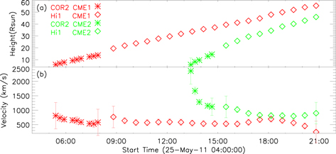
Figure 4. Top: height–time profile for CME-1 (red) and CME-2 (green) based on GCS fits. Bottom: velocity–time profile for CME-1 (red) and CME-2 (green) derived from the measured height in GCS model. The star and diamond symbols show the data from COR2 and HI1 FOV, respectively. The errors on the velocities are derived from the errors of measured heights, 0.5 R⊙ in COR2, and 1.0 R⊙ in HI1 FOV.
Download figure:
Standard image High-resolution imageTable 1. GCS Model Parameters for CME-1 and CME-2
| STEREO A Time | Longitude | Latitude | Tilt Angle | Height | Aspect Ratio | Half Angle | Electron Density Factor |
|---|---|---|---|---|---|---|---|
| (1) | (2) | (3) | (4) | (5) | (6) | (7) | (8) |
| CME-1 | |||||||
| 2011 May 25 05:24 | 5 | −5 | −73 | 5.9 | 0.2 | 10 | 100,000 |
| 2011 May 25 07:24 | 5 | −5 | −73 | 12.5 | 0.22 | 10 | 35,000 |
| 2011 May 25 11:29 | 5 | −12 | −73 | 27.8 | 0.3 | 30 | ⋯ |
| 2011 May 25 15:29 | 5 | −12 | −73 | 39.5 | 0.3 | 30 | ⋯ |
| 2011 May 25 19:29 | 5 | −12 | −73 | 52.0 | 0.3 | 30 | ⋯ |
| 2011 May 25 20:49 | 5 | −12 | −73 | 55.5 | 0.4 | 30 | ⋯ |
| CME-2 | |||||||
| 2011 May 25 13:24 | 8 | 11 | 65 | 5.8 | 0.17 | 8 | 200,000 |
| 2011 May 25 14:39 | 8 | 11 | 65 | 14.0 | 0.18 | 8 | 100,000 |
| 2011 May 25 18:09 | 8 | 5 | 65 | 34.5 | 0.2 | 12 | ⋯ |
| 2011 May 25 20:49 | 8 | 5 | 65 | 46.0 | 0.2 | 12 | ⋯ |
Download table as: ASCIITypeset image
Here, we provide possible explanations to this question. One obvious cause of the problematic CME is the projection effect for the small size of the CME. From the measurement, we find that the half angle (Table 1, column 7) and the aspect ratio (Table 1, column 6) of CME-1 is very small. As a consequence, the main body of CME-1 is obscured by the occulter in the LASCO C2/C3. Nevertheless, from the simulation shown in Figure 3, a small part of the CME-1 still extrudes beyond the occulter of LASCO C2, thus it should have been visible when CME-1 passes beyond the STEREO COR2 FOV. We argue here that the second additional cause of the invisibility is the weak brightness of the CME-1, i.e., the CME-1 brightness is below the background noise level, or the detection threshold of the instrument as demonstrated below.
To calculate the observed brightness of CME-1, we first calibrate STEREO/COR2 images to the customary units of mean solar brightness. After the calibration, the background F-corona, static K-corona, and any residual stray light still remains. The best way to remove these factors is to subtract from the base image (∼04:39 UT), which is prior to the appearance of CME-1 (e.g., Vourlidas et al. 2010). Thus, the leftover brightness changes in the CME-1 region are caused by CME-1. The CME-1 region can be obtained according to the projected shape in GCS model and the occulter edge. CME-1's average observed brightness is calculated by averaging all pixels brightness inside the CME-1 region.
We can also use GCS model to simulate the CME-1 brightness by adjusting three parameters, electron density factor (Ne), Gaussian width of the density profile in the interior (σtrailing) and exterior (σleading) to simulate the electron density distribution of CME. The maximum value of electric density is focusing on the outer surface of shell, and the density falls off in each side according to different Gaussian profile (Thernisien et al. 2006). We have adjusted the input Ne to make the simulated brightness and the observed brightness in the same magnitude, in the visible area of the FOV of STA and STB COR2. As shown in Figure 3, at 07:24 UT, when the value of Ne is 35,000, the average simulated brightness and the observed brightness in CME-1 region are both ∼10−12 B⊙, where the B⊙ is the solar brightness. The values of Ne are listed in Table 1, column 8. The Ne is decreasing as CME-1 propagates in response to its expansion. Taking into account the propagating direction, 3D shape, and maximum electron density of the CME-1, we can calculate the expected CME brightness just outside of the occulter in the FOV of SOHO/LASCO. At 07:24 UT, the expected mean and maximum brightness within the projected area of CME-1 are ∼5.4 × 10⁻¹² B⊙ and ∼1.4 × 10⁻¹¹ B⊙ in the FOV of LASCO C2. On the basis of the design parameters of LASCO coronagraph, the brightness range of C2 is 2 × 10⁻⁷ ∼ 5 × 10⁻¹⁰ B⊙. And for C3, the brightness range is 3 × 10⁻⁹ ∼ 1 × 10⁻¹¹ B⊙ (Brueckner et al. 1995). The expected values of brightness of CME-1 are lower than the detectable brightness range in the SOHO/LASCO C2. The values of simulated and observed brightness are listed in Table 2. The CME-1 may be too diffuse to be observed by SOHO/LASCO coronagraph with finite sensitivity. Hence, there is no corresponding halo CME that can be detected in LASCO C2. The third row of Figure 3 shows the simulated CME brightness distribution, using the local density method in the GCS model (Thernisien et al. 2011, 2006). The expected brightness of CME-1 in SOHO/LASCO from model is much larger than the actual brightness. Because of the different detection thresholds of different instruments, we have to emphasize that the simulated brightness images of CME in the third row of Figure 3 only show the ideal cases, but do not reflect the brightness in real observations when noises are added.
Table 2. The Simulated and Observed Brightness of CME-1
| STEREO A Time | STA Observed | STA Simulated | STB Observed | STB Simulated | SOHO Expected Mean | SOHO Expected Maximum |
|---|---|---|---|---|---|---|
| Brightness(e − 12 B⊙) | Brightness (e − 12 B⊙) | Brightness(e − 12 B⊙) | Brightness(e − 12 B⊙) | Brightness (e − 12 B⊙) | Brightness (e − 12 B⊙) | |
| 2011 May 25 05:39 | 13.9 | 19.1 | 11.0 | 9.18 | 10.3 | 48.0 |
| 2011 May 25 05:54 | 11.9 | 15.6 | 9.53 | 9.67 | 15.6 | 43.5 |
| 2011 May 25 06:24 | 8.35 | 7.48 | 6.82 | 6.80 | 11.3 | 35.2 |
| 2011 May 25 06:39 | 6.79 | 5.68 | 5.60 | 5.10 | 10.5 | 29.7 |
| 2011 May 25 06:54 | 5.04 | 3.94 | 4.18 | 4.11 | 8.07 | 21.4 |
| 2011 May 25 07:24 | 3.30 | 1.53 | 2.77 | 2.57 | 5.47 | 13.6 |
| 2011 May 25 07:39 | 2.65 | 0.69 | 2.24 | 2.40 | 4.45 | 11.7 |
| 2011 May 25 07:54 | 1.64 | 0.27 | 1.40 | 1.93 | 2.79 | 7.88 |
Download table as: ASCIITypeset image
3.2. The Observation and Analysis of CME-2 on 2011 MAY 25
CME-2 was associated with a small filament eruption, originating from a decayed active region at S18°W25°, a different region but very close to the source region of CME-1. CME-2 has also been listed in Nitta & Mulligan (2017) as stealthy CME. Figure 2(b) shows the source region of CME-2 associated PEA. The green line in panel (b) shows the orientation of PEA axis, and the tilt angle of the axis is about 50°. CME-2 first emerged in the FOV of STEREO/COR2 at 13:39 UT, about 8 hr after the first appearance time of CME-1 in the same coronagraph. Data from COR2 coronagraphs, which provide limb views of CME-2, greatly help us limit the first appearance time of CME-2 in SOHO/LASCO coronagraph. When the eruption time of CME-2 is determined, we retrospectively checked the coronagraph observation from SOHO/LASCO and the CDAW LASCO CME catalog. We found a corresponding eruption in the FOV of SOHO/LASCO C2, which is a very faint and diffuse CME moving toward northward. The STB/COR2, SOHO/C2, and STA/COR2 (from left to right) base-difference white-light images for CME-2 at 13:54 UT (subtracted from the corresponding base images at 12:24 UT) are shown in the first row of Figure 5. The projected angular width of CME-2 in LASCO C2 is 78°, as shown in the middle column of row 1 of Figure 5. Using SOHO/LASCO observations alone, we are only with lower confidence as to its link to the problematic ICME. Its nature of Earth-affecting is only revealed retrospectively when STEREO observations are first examined.
Figure 5. Observational and simulated images of CME-2 from three different viewing angles. The panels are similar to those in Figure 2. The first row shows the base-difference images from STEREO A COR2 (left column), SOHO C2 (middle column), and STEREO B COR2 (right column). The second row shows the same images as the first row, but with the GCS model fitting results overlaid (green mesh). The third row shows the schematic simulated brightness images of CME2. A supplementary movie showing the CME2 and the mesh is provided.
(An animation of this figure is available.)
Download figure:
Video Standard image High-resolution imageWhen the outlines of the GCS model matched the outer edges of CME-2 in all three views of white-light coronagraphs, the propagation longitude and latitude of CME-2 are found to be W5°, N12°, apparently an Earth-directed CME. The derived parameters from GCS model are shown in Table 1. The tilt angle of CME-2 is 65°, consistent with the axial orientation of the post-eruption arcade. The aspect ratio of CME-2 is only 0.17, and the half angle is 8°. Because of the small aspect ratio, the projected shape of the CME is an elongated ellipse instead of a circular shape. When the northern part of CME-2 is extruding beyond the occulter, the projected width of CME-2 is still less than the diameter of the occulter, as shown in the second row of Figure 5. As CME-2 continues to expand during its propagation, its electron density decreases. Further, the propagating direction of CME-2 is nearly normal to the plane of the sky in the FOV of LASCO C2/C3. According to the effect of Thomson scatter sensitivity to the viewing angles, the observed intensity is expected to decrease rapidly with distance. When the width of CME-2 becomes larger than the diameter of occulter, i.e., a presumed halo CME, the brightness of CME-2 shall go less than the detectable range of LASCO. As observed after 15:00 UT, the CME-2 front is too faint to be tracked in the FOV of LASCO C2, when the 3D height of CME-2 is about 15 R⊙.
3.3. The Interaction of Two CMEs in the Interplanetary Space
Both CMEs can be well tracked in the FOV of STEREO COR2 and HI1. According to the observations from STEREO, the actual height of CME-1 and CME-2 can be obtained from fitting the GCS model with an error of 0.5 R⊙ in COR2 and 1.0 R⊙ in HI1 FOV. The profiles of actual propagating heights and associated velocities for the CME-1(red points) and CME-2 (green points) are shown in Figure 4. The star symbols show the data from STEREO COR2 and the diamonds for HI1 data, respectively.
Based on coronagraph observations near the Sun, it is expected that CME-1 and CME-2 would interact at a certain distance in the heliosphere. The temporal separation between the launching times of CME-1 and CME-2 is about 8. The directions of propagation of CME-1 and CME-2 are similar. The velocity of CME-1 is almost constant, about 800 km s−1, while for CME-2, it shows a clear decreasing velocity profile, from the velocity of 1670 km s−1 at 13:39 to 821 km s−1 at 20:09. The propagation directions of CME-1 and CME-2 are both within 10° of the Sun–Earth line. Therefore, the two CMEs are expected to interact with each other in the interplanetary space. Such interaction can be further inferred from STEREO/HI observations, as discussed below.
The J-maps, or elongation-time maps (Sheeley et al. 1999), which are stacking running difference slices of COR2, HI1, and HI2 along the ecliptic latitude, are used to track the CME trajectory in the heliosphere. By delineating the enhanced density region in the heliosphere, we have manually constructed the elongation-time profiles for both CME-1 and CME-2 (Figure 6), which are shown as the red line and green line overlaid on the maps. The black horizontal line shows the elongation angle of the Earth. CME-1 and CME-2 could be identified unambiguously up to 15° elongation angle for both STA and STB J-maps. At about 10° elongation angle, one can notice that CME-2 is nearly approaching and catching up with CME-1. After the interaction, CME-2 became faint, and one can only track a single bright leading front out to 35° and 20° elongation in STA and STB, respectively. The propagation longitude of CME-1 and CME-2 is almost same, about 5° west of the Sun–Earth line. The supplemental movies show better interaction between CME-1 and CME-2 in projected images of STEREO. These observations suggest that CME-1 and CME-2 have an interaction with each other in the FOV of HI. Wood et al. (2017) also mentioned that the faster CME-2 catches up to, and slightly overtakes, CME-1 in the HI1 FOV in the appendix event No. 17. As a consequence of interactions, an in situ instrument could observe ICMEs which are merged individual CMEs.
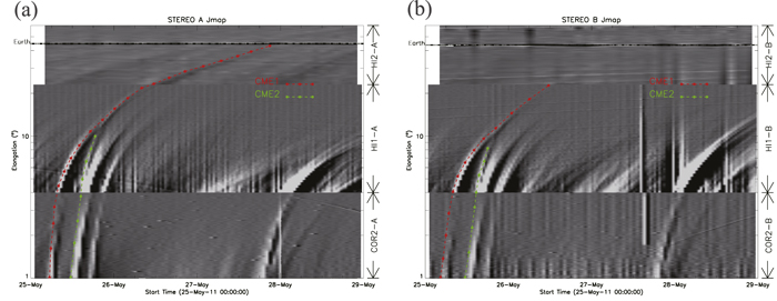
Figure 6. Merge of CME-1 and CME-2 in the interplanetary space. Panels (a), (b) show the J-maps (position angle equal 0) from 2011 May 25 to 29 for STEREO A (left) and B (right) constructed from running difference images of COR2, HI1 and HI2 along the slice on the ecliptic plane. The red and green dashed curves indicate the tracks of CME-1 and CME-2, respectively. The black horizontal line indicates the elongation angles of Earth.
Download figure:
Standard image High-resolution image4. Analysis of in situ Plasma and Magnetic Field Observations
Based on the near-central-meridian source locations of CME-1 and CME-2 and their propagation direction, both CME-1 and CME-2 are likely to impact the Earth along the Sun–Earth line. There is significant doubt as to which of the two progenitor CMEs is responsible for the problematic ICME. Wood et al. (2017) considered the CME-1 is the corresponding CME of the problematic ICME and the CME-2 just barely missing Earth to the west. However, Nitta & Mulligan (2017) considered the CME-2 is responsible for the problematic ICME. According to our simulation results from GCS model, we prefer both CME-1 and CME-2 can arrive at the Earth. Gosling (1990), Webb et al. (2000a), Möstl et al. (2012), and Zhang et al. (2013) argued that a majority of CMEs arriving at Earth should contain a magnetic flux-rope structure. When both CME-1 and CME-2 impact Earth, there should exist two magnetic flux ropes in the in situ observations. To distinguish the corresponding flux ropes of the two progenitor CMEs, we revisit the in situ observations.
As we mentioned in Section 2, there is an interesting short interval in the ICME event with bumpy magnetic field strength and direction, abnormally increased proton temperature, and proton plasma β. We now believe that this short interval is the interaction region between the two magnetic flux ropes. The identification of such an interaction region is also made by Wang et al. (2003) and Mishra et al. (2015) for two interacting CMEs. Based on both in situ and remote-sensing observations, we argue that the recognized ICME is a complex event combined by two magnetic flux ropes concatenated together; the two magnetic flux ropes originate from CME-1 and CME-2, respectively.
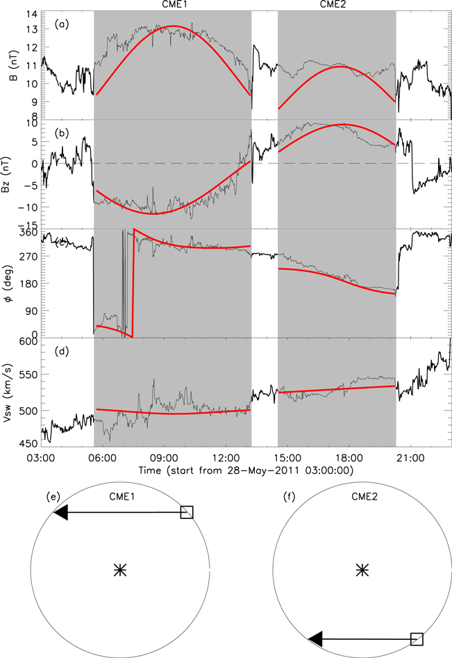
In our analysis, we divide the ICME into two flux ropes as shown in Figure 7. We use a velocity-modified cylindrical flux-rope model with the Lundquist solution developed by Wang et al. (2015) to fit the two independent flux ropes. Figure 7 panels (a)–(d) show the observations from WIND spacecraft at 1 au. The two gray regions mark the intervals of the two flux ropes as FR-1 and FR-2, corresponding to CME-1 and CME-2 in heliosphere, respectively. The overlaid red curves in those panels present the best-fitted results of the velocity-modified models for FR-1 and FR-2. The FR-1 arrived at Earth at 05:34 UT on 2011 May 28, with an impacting velocity of 500 km s−1. Applying the velocity-modified model to FR-1, we deduce the field intensity at the axis is 17.9 nT. The fitted radius of FR-1 is only 0.052 au, which is much smaller than the radius (∼0.1 au) of a typical magnetic cloud (Gopalswamy et al. 2015; Wang et al. 2015). The orientation of the fitted FR axis has a longitude of 217° and latitude of −49°, which is different (∼24°) from the fitted tilt angle of CME-1. This difference can be caused by the uncertainty in the fitting routine, or the possible change of the orientation when the flux rope propagates in the interplanetary space.
Figure 7. In situ solar wind data of CME-1 and CME-2 and their flux-rope model fitting results. From top to bottom, panels (a)–(d) are total magnetic field strength (B), z-component of the magnetic field in GSM coordinate system(Bz), the azimuthal (ϕ) angles of the field direction in GSM coordinate system, and solar wind velocity (V). The two gray shaded regions show the time intervals of CME-1 and CME-2, respectively. The red lines in panels (a)–(e) show the flux-rope fitting results of the two CMEs. Panel (e) and (f) show the satellite paths (arrows) through the fitted magnetic flux ropes.
Download figure:
Standard image High-resolution image
The velocity-modified cylindrical flux-rope model can also simulate the path of the WIND satellite through the flux-rope structure in the coordinate of flux rope. As shown in panel (e) and (f), the circles show the normalized cross-section of the flux ropes. The asterisk in each circle indicates the axis of flux ropes, and the arrow indicates the path of the spacecraft passing the cross-section of the flux rope. For FR-1, the satellite passes the flux rope in the northern part, consistent with the southward propagating direction of CME-1.
The FR-2 arrived at Earth at 14:31 on 2011 May 28, with an impacting velocity of 540 km s−1, which is consistent with the duration of the CME-2 propagation. The axial magnetic field strength of FR-2 is 16.5 nT, and the fitted radius is 0.054 au, also belonging to a small flux-rope category. The fitted latitude and longitude of the FR axis are 60° and 351°, respectively. The orientation of FR-2 inferred from the in situ observation is consistent with the tilt angle (65°) of CME-2 obtained by the GCS model and the corresponding post-eruption arcade axial orientation of 65°. The simulated satellite path through the flux rope is in the southern part, consistent with the propagation direction of CME-2 (W5°, N12°). Compared with the observational solar wind data, the normalized root-mean-square (rms) of the difference between the modeled results and observations is 0.21 and 0.25 for FR-1 and FR-2, respectively, indicating a good fitting. We believe the FR-1 and FR-2 are corresponding to the CME-1 and CME-2 in the coronagraph. The two flux ropes subsequently caused a moderate geomagnetic storm, with the Dstmin = −80 nT.
5. Conclusion and Discussion
In this paper, we propose the concept of problematic ICMEs, i.e., ICMEs clearly identified by in situ observations near Earth have no associated progenitor halo CMEs seen from coronagraphs situated along the Sun–Earth line. With the assistance of STEREO observations, we answer the question why there is no visible halo CME in SOHO/LASCO observations for a problematic ICME occurred on 2011 May 25. We attribute the causes of stealth to two factors: (1) the projection effect of Earth-directed small-size CMEs with the projected area mostly behind the occulter, and (2) the low brightness of CMEs below the detection threshold of instruments. There are two progenitor CMEs (CME-1 and CME-2) identified from STEREO observations. The propagating direction of CME-1 and CME-2 are both along the Sun–Earth line. CME-1 is invisible in the FOV of SOHO/LASCO, while CME-2 is recognized as a northward narrow CME instead of a halo CME. Due to the small aspect ratio (or small cross-section size) and small angular width of CME-1, CME-1 has to propagate to a far distance in order to be imaged beyond the occulter of LASCO. When CME-1 went beyond the occulter, its brightness was less than the detectable brightness threshold of LASCO C2 and C3. Hence, CME-1 was too diffuse to be detected as halo CME. The propagating direction of CME-2 is N12° W5°. Because of the small aspect ratio, the initial projected width of CME-2 is less than the diameter of the occulter. Only the northern part of CME-2 went beyond the occulter, appearing as a narrow northward CME. When the projected width of CME-2 is larger than the diameter of the occulter, CME-2 is too weak to be visible.
By determining the velocities of CME-1 and CME-2, we infer that CME-1 and CME-2 interact with each other in the interplanetary space, which is also supported by heliographic imaging observations. We reveal that the in situ ICME is a complex ejecta containing two magnetic flux-rope structures. The sizes of FR-1 and FR-2 are smaller than the typical magnetic cloud, belonging to the category of small/moderate scale flux ropes. There is an ambiguity in where small/moderate flux-rope structures are formed (Moldwin et al. 2000; Feng et al. 2007). Our analysis associated the two in situ observed small/moderate flux ropes with the progenitor CMEs in the remote imaging observations in the FOV of STA and STB COR2. The study provides direct evidence to support the idea that small/moderate scale flux ropes are interplanetary manifestations of small CMEs originating from the Sun.
Our analysis suggests that our ability to identify the progenitor CMEs was limited by the sensitivities of the instruments and projection effects. There are some ICMEs identified by in situ observations near Earth that are associated with extremely well-observed partial or full halo CMEs in coronagraphs on board SOHO, and also there are some well-identified ICMEs associated with very poorly observed progenitor CMEs. Our study confirms that in reality problematic ICME is nothing more than one end of this spectrum. Therefore, we emphasize that classification of problematic ICME is merely an observational one. We do not categorize the occurrence of problematic ICMEs as a phenomenon that has different physics from other types of regular ICMEs. We believe that the progenitor CMEs for regular ICMEs or problematic ICMEs probably have no difference in fundamental physics of eruption from the Sun.
Predicting the hit/miss and the time of arrival of CMEs is one of the most important problems of space weather science. The Earth-affecting CMEs usually appear as a halo (full halo or partial halo) CME in the FOV of coronagraphs located near the Earth, such as SOHO/LASCO. However, the existence of problematic ICMEs poses a challenge for space weather prediction. We think that there are two effective ways to find the corresponding progenitor CMEs near the Sun for these problematic ICMEs. First, it is to improve the sensitivity of instrumentations to reduce the detectable brightness threshold. Second, to get rid of the intrinsic limits of the projection/occulting effect, Earth-directed CMEs are much more easily detected by coronagraphs off the Sun–Earth line. Our study emphasizes the importance of having permanent observations from satellites off the Sun–Earth line, such as L4 or L5 missions.
We acknowledge the use of data from the SOHO, STEREO, and Wind spacecraft. STEREO is the third mission in NASA's Solar Terrestrial Probes program, and SOHO is a project of international cooperation between the ESA and NASA. This work is supported by NSFC 41774181 and Youth Innovation Promotion Association CAS. J.Z. is supported by US NSF AGS-1249270 and NSF AGS-1156120.