


Abstract
We have surveyed the Voyager magnetic field data from launch through 1990 in search of low-frequency waves that are excited by newborn interstellar pickup ions (PUIs). During this time the Voyager 1 and 2 spacecraft reached 43.5 and 33.6 au, respectively. The use of daily spectrograms permits us to perform a thorough search of the data. We have identified 637 different data intervals that show evidence of waves excited by either pickup He+, H+, or both, and these intervals extend to the furthest distances in the years studied. To compare wave features against more typical interplanetary observations, we also employ 1675 data intervals spanning the same years that do not contain wave signatures and use these as control intervals. While the majority of wave events display the classic spectral characteristics of waves due to PUIs, including left-hand polarization in the spacecraft frame, a significant number of the events are right-hand polarized in the spacecraft frame. We have no complete explanation for this result, but we do show that right-handed waves are seen when the local magnetic field is nonradial.
Export citation and abstract BibTeX RIS
1. Introduction
Neutral atoms can reach into the interplanetary medium from numerous sources including interstellar space, comets, dust, and planetary atmospheres. For the most part, they pass through the solar wind without significant interaction until they are ionized by one of several processes. Once ionized, their motion is dictated by the heliospheric magnetic field (HMF), the solar wind, and the processes within interplanetary space that lead to acceleration of the newborn ion. Only a few spacecraft possess the instrumentation to make direct measurements of the neutral atom or the newborn ion. This paper focuses on observations of magnetic waves seen by the Voyager spacecraft from launch in late 1977 through 1990 that are excited by newborn pickup ions (PUIs) in the solar wind, which are argued to originate as neutral interstellar atoms. The Voyager spacecraft lack detectors that are capable of making direct measurements of the PUIs, so the analysis of the waves they produce provides the most direct measure of their existence and properties.
Waves due to newborn interstellar PUIs have been previously reported using observations by the Ulysses (Murphy et al. 1995; Cannon et al. 2013, 2014a, 2014b, 2017), ACE (Argall et al. 2015; Fisher et al. 2016), and Voyager 1 and 2 (Joyce et al. 2010, 2012; Aggarwal et al. 2016; Argall et al. 2017) spacecraft and are reviewed in Smith et al. (2017). Interstellar neutral hydrogen (H) is argued not to penetrate the heliosphere inside ∼3 au, as ionization of the neutrals is adequate to reduce their density to negligible levels inside this range. Therefore, ACE observations of waves due to interstellar PUIs are limited to He+ source ions. To date, Ulysses data have been examined only for the expected H+ source. Preliminary surveys of the Voyager 2 observations have revealed waves due to both He+ and H+ ions.
The waves that are excited by the newborn interstellar PUIs cannot persist indefinitely. Their energy is argued to be absorbed by the nonlinear processes that form the interplanetary turbulence and transported to small scales where various dissipation processes act to convert the energy into heat (Zhou & Matthaeus 1990a, 1990b; Matthaeus et al. 1994; Williams & Zank 1994; Richardson et al. 1995, 1996; Williams et al. 1995; Zank et al. 1996, 2012, 2017; Smith et al. 2001, 2006b; Isenberg et al. 2003, 2010; Richardson & Smith 2003; Breech et al. 2005, 2008, 2009, 2010; Isenberg 2005; Oughton et al. 2006, 2011; Ng et al. 2010; Usmanov et al. 2012, 2014a, 2014b; Adhikari et al. 2015a, 2015b, 2017). Direct measurement of the turbulent transport of energy within the inertial range has been shown to be in agreement with the inferred heating rate of thermal protons in the solar wind (MacBride et al. 2008; Stawarz et al. 2009; Coburn et al. 2012). The waves excited by newborn interstellar PUIs form an additional energy source that is critical to explaining the observed solar wind temperature beyond ∼20 au. Likewise, it has been argued that the waves cannot be observed if the rate of energy transport by the turbulence exceeds the rate of wave growth (Cannon et al. 2014b; Aggarwal et al. 2016; Fisher et al. 2016; Smith et al. 2017). When this happens, the wave energy is still produced by the PUIs, but is absorbed into the turbulent transport too quickly to allow the waves to reach observable amplitudes.
We examine here Voyager data from launch in late 1977 through 1990 in an effort to extend the initial discoveries of waves due to newborn interstellar PUIs found previously in the Voyager observations (Joyce et al. 2010, 2012; Aggarwal et al. 2016; Argall et al. 2017). This will extend the past survey for such waves out to 43.5 au for Voyager 1 and 33.6 au for Voyager 2. We follow an established approach using techniques and tools that have already resulted in similar observations in the Ulysses and ACE data sets (Cannon et al. 2014a, 2017; Argall et al. 2015, 2017; Fisher et al. 2016). These techniques have enabled us to build an extensive catalog of 637 wave events in association with pickup He+ and H+ that have been recorded by the Voyager 1 and 2 spacecraft. Here, we present a systematic analysis of these events, including polarization parameters, wave power, minimum variance directions, and a detailed analysis of the plasma conditions when the waves are observed. In a companion paper (Hollick et al. 2018b) we compute wave growth rates that we compare against turbulence rates in an effort to describe the variation in local turbulence conditions that permit the waves to reach observable levels.
2. Theory
The pickup process begins with a neutral atom moving at ∼25 km s−1 relative to the Sun, a velocity that is commensurate with the motion of the heliosphere through the interstellar medium (Bzowski et al. 2012, 2015; McComas et al. 2012, 2015, 2017; Möbius et al. 2012; Schwadron et al. 2015). The newborn ion's velocity within the rest-frame of the solar wind (where the nominal solar wind speed VSW ∼ 450 km s−1) is converted into cyclotron motion across the local magnetic field and streaming along the local magnetic field according to the orientation of the HMF at the point of ionization. Ionization is accomplished primarily by two methods: photoionization by solar EUV and collision with solar wind protons. He+ is produced primarily by photoionization, while H+ production includes a significant collisional component.
Because the newborn ion's speed in the plasma frame is essentially the same as the solar wind speed, which is ∼10 × the Alfvén speed, the waves that are excited by the ions are seen at frequencies in the spacecraft frame  , where
  is the ion cyclotron frequency, ei is the ion charge, B is the magnetic field magnitude, mi is the ion mass, and c is the speed of light. Scattering the PUI to larger pitch angles reduces the distance the ion streams along the mean magnetic field in one gyroperiod and shifts the resonance condition to higher wavenumbers, which are seen at higher frequencies in the spacecraft frame. Wave excitation at
  requires particle energization (Lee 1983; Kennel et al. 1986; Smith 1989; Bamert et al. 2004) and while PUIs may be accelerated at shocks or in other regions (Gloeckler et al. 2005), acceleration is not part of the general description of the pickup process (Gloeckler et al. 1993; Zank 1999).
Ionization of neutral H is relatively efficient, so very little gets inside ∼3 au (Zank 1999). This makes excitation of energetically significant wave activity by newborn interstellar H+ inside ∼3 au very unlikely (Joyce et al. 2010; Cannon et al. 2014a, 2014b; Aggarwal et al. 2016). In contrast, interstellar neutral He reaches deep within the inner heliosphere and is gravitationally focused behind the Sun (Gloeckler et al. 2004). The resulting waves have been seen at 1 au (Argall et al. 2015; Fisher et al. 2016).
Newborn PUIs in a radial magnetic field stream sunward through the solar wind at speeds greater than the Alfvén speed. This excites a resonant beam instability of sunward-propagating fast-mode waves that are right-hand-polarized in the plasma frame. Particle-scattering to greater pitch angles results in the excitation and damping of various low-frequency modes, but the asymptotic state consists of right-hand-polarized, sunward-propagating waves that are seen as left-hand-polarized at  in the spacecraft frame (Lee & Ip 1987).
3. Analysis Overview
We analyze magnetic field data from the Voyager 1 and 2 spacecraft from launch in late 1977 through 1990 (Behannon et al. 1977) and augment this analysis with thermal proton data from the PLS instrument (Bridge et al. 1977). In this time the Voyager 1 (V1) spacecraft reaches 43.5 au and 31.3° of heliolatitude. The Voyager 2 (V2) spacecraft is sent to Uranus and Neptune following the Saturn encounter and therefore remains more nearly within the ecliptic plane, reaching 33.6 au by the end of 1990. Figure 1 shows the trajectories of the two spacecraft over these years. Planetary encounters for Jupiter (J), Saturn (S), Uranus (U), and Neptune (N) are marked in the second panels.
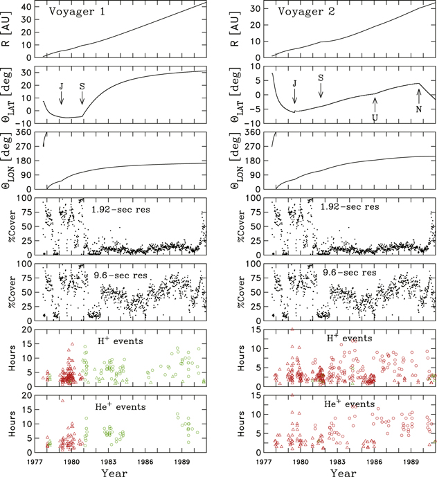
Figure 1. Trajectory of the Voyager 1 (left) and Voyager 2 (right) spacecraft from launch through 1990. (Top to bottom) R is the heliocentric distance (from the spacecraft to the Sun), ΘLAT is the heliolatitude, and ΘLON is the heliolongitude. The times of closest approach for Jupiter (J), Saturn (S), Uranus (U), and Neptune (N) are marked in the ΘLAT panels. The percent of data available in any given 5-day file is plotted for 1.92 and 9.6 s data resolutions. The times when waves are due to pickup He+ and H+ are shown along with the duration of the wave events (red denotes wave events with PLS data and green denotes wave events without PLS data.
Download figure:
Standard image High-resolution imageThe National Space Science Data Center (NSSDC) provides magnetic field data from the Voyager spacecraft at four cadences: 1.92, 9.6, 48 s; and 1 hr. Data files typically span five days. Figure 1 shows the average daily percent coverage for magnetic field data in the 1.92 and 9.6 s data files. Coverage is not the same for all data rates. Both 9.6 and 48 s data have more complete coverage than the 1.92 s data, and this is especially true after the start of 1981. For this reason, and because longer data intervals are needed to yield spectra at lower frequencies, we use the 9.6 s data to augment the 1.92 s data when the latter are incomplete. Beyond the start of 1981, the HMF intensity B is low enough to permit the resolution of the proton cyclotron frequency and associated waves using this lower cadence data. We do not use the 48 s, as the coverage is no better than that for the 9.6 s data and it provides a lower Nyquist frequency making resolving the waves more difficult.
The bottom two panels of Figure 1 also show the times of wave observations associated with pickup H+ and He+, along with the duration of the events. The red (green) symbols represent times when thermal proton data such as wind speed and proton density are available (unavailable) from the PLS instrument. The triangles (circles) represent the 1.92 s (9.6 s) data. We follow this convention throughout the paper. The event durations may be limited by data availability, as is the ability to find events. It is likely that the 50% coverage of the 9.6 s data after 1981 implies that there are actually twice as many wave intervals in these years at the spacecraft location than we are able to find in the data. Typical event durations are under 10 hr and very often under 5 hr. This does not reflect the lifetime of the event in the plasma. It is only a measure of the size of the plasma region that contains the waves and the time it takes that region to pass over the spacecraft. Actual lifetimes of the wave events may be longer. Years without any apparent wave events were examined and none were found. A detailed list of the event times and locations is available in Hollick et al. (2018a). A total of 637 intervals of Voyager magnetic field data containing waves due to PUIs were used in this study. The number of events of each type used is listed in Table 1. The two events examined by Argall et al. (2017) were not included in this study.
Table 1. Number of Wave Intervals Used
| S/C | Cadence | Ion | PLS | Number |
|---|---|---|---|---|
| (s) | Y/N | |||
| V1 | 1.92 | He+ | Y | 46 |
| V1 | 1.92 | He+ | N | 5 |
| V1 | 9.6 | He+ | Y | 0 |
| V1 | 9.6 | He+ | N | 49 |
| V1 | 1.92 | H+ | Y | 129 |
| V1 | 1.92 | H+ | N | 26 |
| V1 | 9.6 | H+ | Y | 0 |
| V1 | 9.6 | H+ | N | 71 |
| V2 | 1.92 | He+ | Y | 75 |
| V2 | 1.92 | He+ | N | 2 |
| V2 | 9.6 | He+ | Y | 54 |
| V2 | 9.6 | He+ | N | 0 |
| V2 | 1.92 | H+ | Y | 248 |
| V2 | 1.92 | H+ | N | 9 |
| V2 | 9.6 | H+ | Y | 77 |
| V2 | 9.6 | H+ | N | 2 |
Download table as: ASCIITypeset image
The analysis begins with daily spectrograms using both 1.92 and 9.6 s magnetic field data to compute the polarization parameters and power levels at the kinetic scales associated with the He+ and H+ cyclotron frequencies. Argall et al. (2017) showed an example of these spectrograms. Daily spectrograms form a necessary basis for finding the wave events because they are relatively rare and do not coincide with easily recognized conditions such as shocks. Both here and in the Ulysses analysis (Cannon et al. 2014a) the waves intervals represent only ∼1% of the total data. In the ACE observations of waves excited by He+ the events form only ∼0.1% of the data. Waves are most readily found by examining the polarization where the signals stand out from the normally unpolarized signals of interplanetary turbulence. The times of these waves are extracted, and the data are run through separate spectral analysis routines using both Blackman–Tukey and FFT algorithms. Comparison of wave spectra against plots of the time series reveal some wave events that may be associated with solar wind transients such as shocks and other dynamics unrelated to this study. These intervals are discarded. We also exclude large intervals of data associated with planetary encounters including their upstream regions on both the inbound and outbound passes (Ness et al. 1979a, 1979b, 1981, 1982, 1986, 1989; Goldstein et al. 1983, 1984, 1985, 1986; Smith et al. 1983, 1984, 1989, 1991; Krimigis et al. 1985), where waves may be generated by ions due to planetary processes, such as bow-shock acceleration, leakage from the magnetosphere, or pickup of planetary neutral atoms. The times of planetary closest approach are shown in the second panels of Figure 1. These times, as well as the associated times excluded from this analysis, are listed in Table 2. Distant Jovian magnetotail encounters continue until the orbit of Saturn (Kurth et al. 1981, 1982), but there are no shock observations to accompany these encounters, no reason to expect a Jovian source for the PUIs at this distance, and no reason to exclude these data intervals from the analysis.
Table 2. Times of Planetary Closest Approach for the Voyager Spacecraft
| S/C | Planet | CA | CA | Exclude |
|---|---|---|---|---|
| Date | Year/DOY | Year/DOY | ||
| V1 | Jupiter | 1979 Mar 5 | 1979/064 | 1979/053-091 |
| V1 | Saturn | 1980 Nov 12 | 1980/317 | 1980/316-321 |
| V2 | Jupiter | 1979 Jul 9 | 1979/190 | 1979/145-264 |
| V2 | Saturn | 1981 Aug 26 | 1981/238 | 1981/226-244 |
| V2 | Uranus | 1986 Jan 24 | 1986/024 | 1986/010-040 |
| V2 | Neptune | 1989 Aug 25 | 1989/237 | 1989/225-250 |
Download table as: ASCIITypeset image
We compute power spectra via Blackman–Tukey spectral techniques (Matthaeus & Goldstein 1982; Leamon et al. 1998a, 1998b; Smith et al. 2006a, 2006c; Hamilton et al. 2008; Markovskii et al. 2008, 2015) where a first-order difference of the measurements is used to pre-whiten the data and reduce the effect of spectral leakage (Smith et al. 1990). The resultant spectra are then corrected using a "post-darkening" algorithm (Chen 1989). The polarization spectra were computed via a FFT of the time series (Fowler et al. 1967; Rankin & Kurtz 1970; Means 1972; Mish et al. 1982). We compute the minimum variance direction to represent the wave vector k. FFT methods were also used to compute the power spectra, which were found to agree with the Blackman–Tukey spectra shown here. These are the same techniques used previously to study magnetic waves due to interstellar PUIs in the ACE and Voyager data sets (Joyce et al. 2010, 2012; Argall et al. 2015, 2017; Aggarwal et al. 2016; Fisher et al. 2016).
The power spectra for the three components of the magnetic field are computed in mean-field coordinates (Belcher & Davis 1971; Bieber et al. 1996) consisting of the component of the fluctuations parallel to the mean magnetic field and two components perpendicular to the mean field. We will show the trace of the power spectral density matrix, along with the power spectrum of the magnetic component aligned with the local mean magnetic field, BZ. The trace spectrum gives the total power in the magnetic fluctuations, while the spectrum of BZ is one indication of the compressive component of the fluctuations. The degree of polarization, Dpol, is the ratio of the polarized power to the total power in the fluctuations. As such it is computed using the field-aligned component of the power spectral matrix. The coherence, Coh, derives from the off-diagonal terms in the power spectral matrix and offers a measure of the cross-component correlation of the fluctuations. The ellipticity, Elip, is the ratio of the minimum to maximum axes of the fluctuation ellipse. We choose to associate the sign of the polarization with Elip such that Elip > 0 (Elip < 0) denotes right-hand (left-hand) polarization in the spacecraft frame and  (Elip = 0) denotes circular (linear) polarization. The minimum variance direction is computed and taken to represent the direction of propagation relative to the mean magnetic field. This analysis is incapable of distinguishing between parallel propagation in the sunward and anti-sunward directions. Therefore, the angle between the minimum variance direction and the mean field,
  is represented below such that 0° ≤ ΘkB ≤ 90°.
Figure 2 shows stacked plots of our spectral analysis for six intervals of Voyager data containing magnetic waves that are attributable to either pickup He+ or H+. In each case the stack from top to bottom is the trace of the power spectral density matrix (upper curve) and the power spectrum of BZ (lower curve), the degree of polarization, the coherence, the ellipticity, and the angle between the minimum variance direction and the mean magnetic field. The spacecraft, days, and times of the analysis are given at the top of each stack. The red lines in the top panels are fits to the background spectra omitting the wave energy enhancements. The He+ and H+ cyclotron frequencies,  and
and  , are shown in the top panels.

Figure 2. Power and polarization spectra for six data intervals when waves due to pickup ions are seen for Voyager 1 (top row) and Voyager 2 (bottom row). In all cases the upper power curve is the trace of the power spectral matrix and the lower power curve is the power in the field-aligned component. Below that are the degree of polarization, coherence, ellipticity, and angle between the minimum variance direction and the mean magnetic field. The days and times of analysis are given above each spectral stack. See the text for explanation.
Download figure:
Standard image High-resolution imageThe top left panel of Figure 2 shows the computed spectra for Voyager 1 observations on 1979/267 from 06:00 to 12:00 UT. The frequencies of interest are  (
( ) for waves due to pickup He+ (H+). There is a clear enhancement above the background level in total wave power associated with pickup H+, but any enhanced power due to He+ is questionable. The trace (total) power is consistently ∼10× the power in the field-aligned component at the frequencies of interest, as is the case for all the examples shown. This implies the waves are largely transverse fluctuations yielding minimum variance directions that are field-aligned, as shown in the bottom panel. Both Dpol ≃ 0.9 and Coh ≃ 0.9, while Elip ≃ −0.9 in the enhanced frequency range, indicating highly polarized and coherent wave signatures that are left-hand-polarized in the spacecraft frame for both the He+ and H+ source.
The top middle panel of Figure 2 shows spectra for Voyager 1 on 1979/354 from 06:00 to 08:15 UT. There are again signatures of wave activity due to both pickup He+ and H+. Wave power enhancements due to H+ appear to be significant, while excess power due to the He+ resonance is minimal. Both again exhibit magnetic fluctuations that are largely transverse to the mean magnetic field. The polarization parameters Dpol ≃ 0.7 and Coh ≃ 0.9, indicating polarized and coherent wave activity at the relevant frequencies. According to the Elip spectrum, He+-excited waves are left-hand-polarized in the spacecraft frame, while the H+-excited waves are right-handed. Right-hand-polarized waves are seen in a large segment of this analysis, as will be shown below. Right-hand-polarized waves due to newborn interstellar PUIs are not currently understood.
The top right panel of Figure 2 shows spectra for Voyager 1 on 1980/085 from 21:00 to 22:30 UT. This is an example of wave excitation by H+ that probably does not include wave excitation by He+. There is some ambiguity in the interpretation, as is sometimes the case in the results we have found and use in this study. The wave signal shows strong Dpol, Coh, and Elip signatures, is left-hand-polarized in the spacecraft frame, and peaks at  , but it extends significantly to
  and into frequencies that would normally be associated with pickup He+ or with the acceleration of pickup H+. Either there is an aspect of He+ scattering and wave excitation that is unclear, leading to a signal peaked near
  , or the pickup H+ has been energized and is thereby producing waves at
  . This seems unlikely, as examination of the hourly averages of PLS data for this time reveal the spacecraft to be in a rarefaction region about 70 hr after an apparent shock crossing. There are no wave observations during the three days between the shock crossing and this wave event. The absence of intervening wave events would seem to make the shock an unlikely source for the waves and any corroborating PUI measurements are unavailable on the Voyager spacecraft. An unambiguous resolution for the source of waves at
  is not possible given the absence of PUI measurements, so we attribute them to pickup He+ in keeping with traditional theory.
The bottom left panel of Figure 2 shows our analysis of Voyager 2 observations on 1983/294 from 20:00 to 22:30 UT. There is a strong signal of left-hand-polarized waves associated with pickup He+ and no indication of wave excitation by H+. The near complete absence of any wave signal at  appears to indicate that only pickup He+ could explain the observation. It is interesting that the wave power peaks at
  and not at
  . This is also seen in other examples.
The bottom middle panel of Figure 2 shows another example of waves due to both pickup He+ and H+. The wave interval was captured by the Voyager 2 spacecraft on 1985/108 from 09:000–12:00 UT. The waves have a strong degree of polarization and coherence and are left-hand-polarized in the spacecraft frame. The fluctuations are largely transverse to the mean magnetic field and have minimum variance directions that are aligned with the mean magnetic field. This could be considered a textbook example of a weak wave event showing both ion resonances.
The bottom right panel of Figure 2 shows an example of right-hand-polarized waves in the frequency range of pickup H+ seen by Voyager 2 on 1985/340 from 19:15 to 21:00 UT. The He+ frequencies are largely unresolved, but those frequencies that are available show no evidence of wave activity due to He+.
4. Voyager 1 Analysis
Figure 3 shows the general plasma parameters averaged over the duration of the individual Voyager 1 wave events. The average magnetic field intensity B and the angle between the average magnetic field and the radial direction ΘBR are computed directly from the 1.92 and 9.6 s data files used in the wave analysis. The average wind speed VSW, average thermal proton density NP, and thermal proton temperature TP are computed from the hourly averages of the PLS data. The thermal proton pressure ratio βP, Alfvén speed VA, and Alfvén Mach number MA are computed from these basic plasma parameter averages. For reference we plot nominal plasma parameters as represented by the solid curves:  nT,
nT,  , VSW = 450 km s−1,
  cm−3, and
  K, where R is the heliocentric distance measured in au. Times when PLS data are unavailable were described to agree with the above thermal proton scalings. These choices are obtained from general scalings of the HMF (Parker 1963) that have been confirmed by observation (Burlaga et al. 2002) and the observed radial scaling of the solar wind speed, density, and temperature (Richardson et al. 1995). It is true that these scalings may not accurately represent conditions when wave events are seen owing to considerations such as stream structure, transients, and latitudinal variation of flow conditions, leading to issues such as flow expansion and the associated reductions in density and temperature, etc. We offer these scalings only to provide a general framework for understanding the results.

Figure 3. Plasma conditions for He+-excited waves (left) and H+-excited wave intervals (right). (Top to bottom) Magnetic field intensity, B; angle between the mean field and radial directions, ΘBR; solar wind speed, VSW; thermal proton density, NP; thermal proton temperature, TP; proton plasma beta, βP; Alfvén speed, VA; and the Alfvén Mach number,  . The curves represent nominal average conditions, as described in the text.
Download figure:
Standard image High-resolution imageThe spectral values of Dpol, Coh, Elip, and ΘkB are averaged over  for both the He+ and H+ cyclotron frequencies. Figure 4 shows the results of those averages for the Voyager 1 wave events. The double-peaked distribution of Dpol when plotted as a function of Elip that is seen for both the He+- and H+-excited waves is the same as was seen for H+-excited waves in the Ulysses measurements (Cannon et al. 2014a). Both the He+- and H+-excited waves show a dominance of left-hand-polarized waves, but there are a large number of right-handed waves. In the Ulysses (Cannon et al. 2014a), ACE (Fisher et al. 2016), and early Voyager analyses (Aggarwal et al. 2016) only ∼10% of the waves were seen to be right-hand-polarized. The early Voyager analyses were limited to observations inside ∼6.5 au. In this analysis the fraction is much larger. Comparison of Dpol and Coh shows a linear correlation between the two measurements for both ion sources. When we plot Elip as a function of heliocentric distance it becomes readily evident that the right-hand-polarized waves are found at R > 5 au, while they dominate at R > 10 au. The fact that the PLS data becomes unavailable for the Voyager 1 observations in this range is not thought to be relevant. Typically, ΘkB < 30°, in generally good agreement with the expectation that the most rapid wave growth is associated with parallel propagation. Note that this analysis is unable to determine propagation sunward or anti-sunward and the two possibilities are treated as equivalent.

Figure 4. (Top) Dpol plotted as function of Elip for Voyager 1 observations of waves due to newborn interstellar pickup He+ (left) and H+ (right). (Second) Coh plotted as a function of Dpol. (Third) Elip plotted as a function of heliocentric distance. Note the tendency for  at increasing R. (Bottom) Angle ΘkB for He+- (left) and H+-excited waves (right) averaged over the same frequencies and plotted as a function of R.
Download figure:
Standard image High-resolution imageWe fit the trace power spectra by omitting the wave signatures to obtain the background spectrum for comparison against the wave properties. In the process, we examine the frequency range  for both the He+- and H+-excited waves to find the frequency at which the measured wave power is greatest relative to the background fit spectrum. Figure 5 (top) shows the spacecraft-frame frequency where the wave power is at maximum above the background spectrum normalized by the ion cyclotron frequency,
  . The peak wave power occurs primarily within
  , as is generally expected (Lee & Ip 1987).
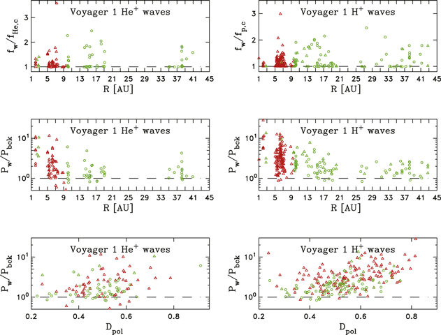
Figure 5. (Top) Ratio of peak wave power frequency to ion cyclotron frequency,  , plotted as a function of R for Voyager 1 observations of waves due to newborn interstellar pickup He+ (left) and H+ (right). (Middle) Ratio of peak wave power to background power level,
  , plotted as a function of R. (Bottom) Ratio of peak wave power to background power level,
  , plotted as a function of degree of polarization Dpol.
Download figure:
Standard image High-resolution imageThe middle panel of Figure 5 shows the maximum wave power, Pw, relative to the background power, Pbck, within the same frequency interval  . This is the wave power at the frequencies shown in Figure 5 (top). There is a clear trend with reduced wave power relative to the background spectrum as the spacecraft moves to greater heliocentric distance. There are many observations with low
  for R < 10 au, but it is in this range that the wave power is greatest. Beyond R = 10 au we see
  as a general rule. This is true for both the He+- and H+-excited waves. At the same time, the bottom panel of Figure 5 shows that
  increases with increasing Dpol, as is expected when adding coherent wave energy to a background spectrum. What could be most interesting is that we have found the polarization spectrum to be a better tool for finding these waves than the power spectrum, as it appears that the polarization develops nonzero values even when the wave power is not seen to significantly exceed the background spectrum. There can be intervals with no discernible excess wave energy, while the polarization spectrum provides a strong signature of resonant activity due to PUIs.
5. Voyager 2 Analysis
We now repeat the above analysis for the wave events recorded by the Voyager 2 spacecraft. We follow the same convention as above where triangles (circles) represent the analysis of 1.92 s (9.6 s) magnetic field data and red (green) symbols represent times when PLS is available (unavailable). Figure 6 shows the plasma parameters averaged over the duration of the individual Voyager 2 wave events. On Voyager 2, PLS data are generally available during these wave events. The field intensity B follows the predicted form with only normal variation. Wave events are not characterized by abnormally high or low values of B. The winding angle ΘBR tends to be smaller than predicted by the Parker spiral. The wind speed is nominal and the proton density is typically less than the prediction. Proton temperatures vary significantly, but do not depart systematically from the predicted value. The measured proton βP tends to exceed the nominal prediction, but is not exceptionally high. The Alfvén speed is nominal to slightly below the prediction and the Mach number MA is correspondingly higher than predicted. Although the measured plasma parameters are often different from the nominal values, the parameters that most systematically depart from expectation are ΘBR and NP. The local mean magnetic field tends to be more nearly radial than the Parker prediction and the proton density tends to be lower than the nominal prediction. These characterizations appear to be equally accurate for both the He+- and H+-excited wave intervals.

Figure 6. Same as Figure 3, but computed for Voyager 2 wave events.
Download figure:
Standard image High-resolution imageFigure 7 reproduces the analyses shown in Figure 4 using the Voyager 2 wave events. The correlation between Dpol and Elip again shows the double-peaked distribution with Dpol peaking at  . Both distributions show a minor peak at Elip ≃ 0 that may bring into question a few of the wave events. The parameters Coh and Dpol are again strongly correlated for both the H+- and He+-excited waves.
  , to a marginal degree. The ellipticity for the He+-excited waves shows a predominance for Elip < 0 that extends out to 35 au. In contrast, there are an approximately equal number of positive and negative values of Elip for the H+-excited waves with little to no clear evidence of a radial trend. As with the Voyager 1 analysis, the angle between the mean magnetic field and the minimum variance direction, ΘkB, for the He+-excited waves increases with R. The H+-excited waves exhibit a broad scatter across the full range of values. There is a tendency for ΘkB < 30° for R < 15 au, but this is not a strong organizer of the observations.
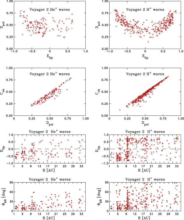
Figure 7. Same format as Figure 4, but showing analysis of Voyager 2 wave data.
Download figure:
Standard image High-resolution imageFigure 8 repeats the analysis of Figure 5 using the Voyager 2 wave events. As before, the peak in the power spectrum is seen close to the associated ion cyclotron frequency with  in most cases. Again, the power associated with that peak becomes a decreasing fraction of the background power at the same frequency as the heliocentric distance increases. This means that the strongest signals in the magnetic power spectrum are at smaller values of R. Also as before, the ratio of wave power to background power where the signal peaks,
  , increases with Dpol. This is not unexpected and simply represents the fact that when the wave signal is stronger it appears in both the power and the polarization spectra.

Figure 8. Same analysis as Figure 5, but applied to the Voyager 2 wave events.
Download figure:
Standard image High-resolution imageIf we compare the Voyager 1 and 2 results, we see they are largely similar. The Voyager 2 event list is longer and benefits from greater availability of PLS data, but otherwise there is relatively little difference in the conclusions. Events arising from H+ resonances outnumber the events due to He+ in both cases. There seems to be little significant results from Voyager 1 climbing to higher heliographic latitudes during this time.
6. Right-hand Polarization
Theory predicts that the asymptotic form of the magnetic spectra for wave excitation by newborn interstellar PUIs is left-hand-polarized in the spacecraft frame (Lee & Ip 1987). However, that analysis assumes a radial mean magnetic field. The winding angle of the Parker spiral approaches 90° beyond ∼5 au with  . Wave instabilities are modified for non-radial fields that result in initial PUI distributions other than field-aligned beams, and instabilities are severely modified for mean fields at right angles to the flow (Gary & Madland 1988; Wong et al. 1991; Gary 1993) that result in non-streaming, gyrating ion distributions. As a possible explanation for the observation of right-hand-polarized waves seen at R > 5 au in Figures 4 amd 7, we compute the angle between the local mean magnetic field and the radial direction, ΘBR, and plot the ellipticity as a function of this angle. Figure 9 shows the results of that analysis. Although there are 10 examples of right-hand-polarized waves due to pickup H+ and 1 example of right-hand-polarized waves due to pickup He+ with ΘBR < 30°, the majority of observations are seen at ΘBR > 30°. This suggests that the instabilities and resulting imbalance between left-hand-polarized and right-hand-polarized wave excitation may be sufficiently modified by the local field orientation to explain the large number of right-hand polarized waves seen here. If true, we must also note that a majority of waves excited by He+ in this range of ΘBR remain left-hand-polarized and at least as many waves due to H+ are left-hand-polarized as are right-hand polarized.

Figure 9. Analysis shows that waves with right-handed ellipticity are seen when the local mean magnetic field is nonradial. Although waves for ΘBR > 30° are not exclusively right-hand-polarized, few right-handed waves are seen for ΘBR < 30°.
Download figure:
Standard image High-resolution imageA second possible explanation for this result could be that field line bending results in viewing the wave in a field orientation that is different from when the wave was excited. This would require that the field line be bent "backwards" after the wave is excited. This seems unlikely, as field line bending would not seem to be a rapid process beyond 5 au and would require that the wave remain excited and unchanged as the field line direction is bent beyond ΘBR = 90°. Thermal electron data would be helpful in addressing this possibility, but is unavailable.
7. Flow Conditions
Figures 3 and 6 demonstrate that the solar wind thermal proton densities appear to be low when the waves are seen. In our companion paper we argue that the background magnetic fluctuations must likewise be low for the waves to be resolved in the data. This can occur under several conditions, including rarefaction regions and interplanetary coronal mass ejections. To demonstrate the role of rarefaction regions in providing the necessary conditions for the wave events to be seen, we compute the gradient of the wind speed about the wave event. We do this by computing the average wind speed from 12 to 24 hr before the start of the event and subtracting this average from that the average of the wind speed computed from 12 to 24 hr after the end of the wave event. This yields a negative value in rarefaction.
Figure 10 shows the results of that analysis. While we continue to adhere to the convention that red (green) symbols represent those events when PLS data is (is not) available for the event times, we must note that PLS data availability for the analysis in this figure does not map one-to-one to PLS data availability for the event times. Since we use data before and after the event time in this analysis, there are events where PLS data are available for the event, but are not available either before or after for use in this analysis. The reverse is also occasionally true. There appears to be a general tendency for ΔVSW < 0, although there are counter examples. As the spacecraft move to greater heliocentric distances the value of ΔVSW approaches zero. This may reflect the general lessening of the wind speed gradient as the rarefaction regions expand or the development of merging regions. It is not our contention to argue that the waves are only seen in rarefaction regions. However, rarefaction regions do appear to play a significant role in providing the necessary low background levels that permit the observation of the waves.

Figure 10. Analysis of solar wind speed changes over a 48 hr period surrounding the wave events. Negative values represent decreasing wind speeds that are indicative of rarefaction regions.
Download figure:
Standard image High-resolution imageFigures 3 and 6 show that the local mean magnetic field during wave events appears to be more radial than the Parker spiral would suggest. This implies that the rarefaction regions that are often associated with the waves may be of the type where the heliospheric field threads the rarefaction (Gosling & Skoug 2002; Murphy et al. 2002; Schwadron 2002; Schwadron & McComas 2005). At 1 au these intervals tend to have nearly radial HMF, but beyond this point we know very little about the evolution of such regions. It may well be the case that the same dynamics that wind the HMF toward  also wind the field away from 0° in these rarefaction regions as the rarefaction region grows in size and the gradient of the flow decreases.
It is interesting to note that the early H+-excited waves inside 2 au, whose existence would appear to be poorly described by newborn interstellar ion theory, are also seen within regions of strongly expanding flow. Our analysis of these events in our companion paper (Hollick et al. 2018b) indicates that the source of these waves cannot be newly ionized interstellar H. It is unlikely that these observations are related to low-frequency wave (LFW) storm events (Jian et al. 2010, 2014; Boardsen et al. 2015; Gary et al. 2016), but the possibility must be admitted. Small-scale magnetic flux ropes have also been found at 1 au that could match the scale of these observations (Zheng & Hu 2018). However, there is evidence of so-called inner-source PUIs, including H+, beyond 1 au (Gloeckler et al. 2000, 2000; Allegrini et al. 2005) and this may be the more likely explanation for these observations. To date, the definitive source is undetermined.
8. Control Analysis
In an effort to compare the properties of wave intervals to times when no waves are present, we have performed the same analyses on 1675 intervals of Voyager 1 and 2 magnetic field data. The number of control intervals of each type is listed in Table 3. These intervals were chosen to be without signatures of waves due to any sources. Otherwise, they were selected only on the basis of having nearly stationary magnetic field and plasma flow conditions without significant discontinuities and possessing well-resolved power-law spectra. In short, they were chosen to be typical of solar wind conditions and suitable for an analysis of interplanetary turbulence. Figure 11 shows the general plasma parameters for these control intervals. Because control intervals do not contain wave signatures, the general plasma parameters are not broken out according to source ion species. The average field intensity, B, proton density, NP, and proton temperature, TP, for the control intervals appear to be better represented by the nominal curves than was found for the wave events. The typical measured values of VA for control intervals appear to be lower than the nominal value shown in the plot while the values of βP appear higher. This likely points to a less than optimal modeling of the nominal solar wind conditions.

Download figure:
Standard image High-resolution imageTable 3. Number of Control Intervals
| S/C | Cadence | PLS | Number |
|---|---|---|---|
| (s) | Y/N | ||
| V1 | 1.92 | Y | 219 |
| V1 | 1.92 | N | 80 |
| V1 | 9.6 | Y | 136 |
| V1 | 9.6 | N | 109 |
| V2 | 1.92 | Y | 309 |
| V2 | 1.92 | N | 9 |
| V2 | 9.6 | Y | 780 |
| V2 | 9.6 | N | 33 |
Download table as: ASCIITypeset image
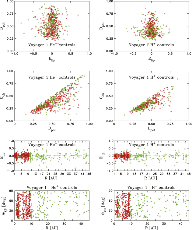
We can repeat the above polarization analyses using the control intervals. Figure 12 shows the analysis of Voyager 1 control intervals. Although there are no clear wave signatures, we repeat the same technique of averaging over the frequency interval  . We again adopt the convention that red (green) symbols represent times when thermal proton data such as wind speed and proton density are available (unavailable) from the PLS instrument and triangles (circles) represent the 1.92 s (9.6 s) data. The double-peaked distribution of Dpol when plotted as a function of Elip that was seen for the wave intervals is no longer present. There is a range of values for Dpol, but Elip adheres to a narrow range about Elip ≃ 0. When Coh is plotted against Dpol the linear scaling seen in the wave events is degraded according to
  . This appears to be a general property of the turbulence that is not seen in the wave events. The control intervals are generally characterized by Elip ≃ 0 and this is seen throughout the range 1 ≤ R ≤ 45 au. There is no trend with R as is seen for the wave events. All of these statements appear to be equally applicable to both He+ and H+ frequencies.
Download figure:
Standard image High-resolution imageFigure 12 also repeats our analysis of ΘkB averaged over the range  for both the He+ and H+ cyclotron frequencies using the Voyager 1 control intervals. Note that when comparing these results to Figure 4 it becomes evident that the wave events show average values of ΘkB that are significantly smaller and less broadly distributed than the control intervals. This, too, appears to be equally applicable to both He+ and H+ frequencies. It appears that the typical turbulence conditions exhibit magnetic fluctuations that are significantly less transverse to the local mean magnetic field than are the waves excited by newborn interstellar PUIs.
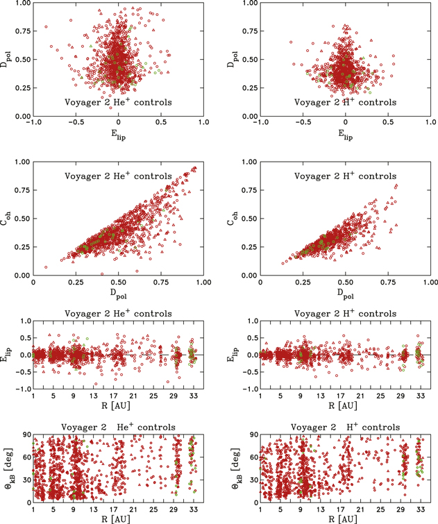
Figure 13 repeats the analysis of Figure 12 using the Voyager 2 control intervals. The conclusions are similar. The value of  , while Dpol varies over the full range of values. The double-peaked distribution of Elip seen for the wave events is not observed. The strong correlation between Dpol and Coh seen in the wave events is degraded to
  , as seen for the Voyager 1 control intervals. The analysis of Elip shows no radial dependence and ΘkB varies extensively between 0° and 90°. The most significant distinctions between the Voyager 1 and 2 control analyses is that the Voyager 2 data set continues to provide thermal proton data and the spacecraft does not leave the ecliptic plane. The polarization analyses appear fully consistent between the two control sets.
Download figure:
Standard image High-resolution image9. Discussion
There are several repeatable spectral features that complicate the identification of sources as pickup He+ or H+. These include:
- 1.Shocks and other potential sources of particle acceleration may produce energetic particles that excite waves at the frequencies of interest here. Normally, these spectra are distinct from what is expected of PUIs, but the possibility of relatively unevolved acceleration, together with questions of energization of PUIs, can complicate the source identification.
- 2.The possible overlap of He+-associated waves with H+ frequencies may provide a false association with H+ ions.
- 3.The possible, but understudied, energization of pickup H+ may result in waves at frequencies
 that could be incorrectly attributed to pickup He+.
 - 4.We have observed waves at that appear to be associated with sources other than pickup H+. These spectral features are often, but potentially not always, disconnected from the expected range of . Until they are better understood, we cannot rule out the possibility that some wave events attributed to pickup H+ are actually due to these other sources.
- 5.A significant number of events studied provide useful information for waves due to pickup H+, but are too short in duration to adequately resolve He+ dynamics.
- 6.There is, to date, no complete explanation for the waves seen to have right-hand polarization in the spacecraft frame. We have shown that these waves tend to be seen when ΘBR > 30°, but left-hand-polarized waves are also seen under these conditions. We suspect there is a different balance between the various instabilities in play under these conditions and we admit that these waves may be due to some form of incomplete PUI scattering. Without better measurements we cannot rule out the possibility of alternative sources.
- 7.In many instances, there is no observable enhancement to the wave power, and determination of PUI dynamics is based solely on polarization spectra. These can be misleading at low frequencies where poor statistics at low frequencies can mimic wave signatures.


There is little that can be done with this potential confusion at this time. We continue to study the observations and may have a better understanding at some time in the future. Readers are invited to study these events and their times are listed in our associated publication (Hollick et al. 2018a).
10. Summary
We have examined Voyager 1 and 2 magnetic field data from launch through 1990 using daily spectrograms in search of waves excited by newborn interstellar pickup He+ and H+. During this time, Voyager 1 and 2 reached 43.5 au and 33.6 au, respectively. A total of 637 wave events were found. Some possess signatures of just one ion source and some possess waves due to both. While the Voyager 1 observations are more numerous at R < 10 au, the distribution of Voyager 2 observations of both wave types is more nearly uniform throughout the entire range of heliocentric distances. Data coverage for the two spacecraft was approximately equal, so this does not seem to explain the difference in event distribution. Latitudinal effects may play a role in determining how often waves are observed, but there are many variables in determining this including solar cycle dependence of ionization rates, frequency of flow conditions, and background turbulence levels. We feel this is beyond what we can accomplish here. While about 10% of wave events seen in the ACE and Ulysses data sets (Cannon et al. 2014a; Fisher et al. 2016) are seen to be right-hand-polarized in the spacecraft frame, which is contrary to theoretical expectations (Lee & Ip 1987), a much larger percentage of the Voyager observations are seen to be right-hand-polarized in the spacecraft frame. We offer no explanation for this other than to note that right-hand-polarized waves are seen when the average magnetic field forms an angle with the radial direction that is greater than 30°. This is expected to alter the balance between the different instabilities that are active for PUI populations and we surmise that incomplete particle-scattering may be partially responsible for the unexpected result.
Theory predicts that the wave normals will be parallel to the local mean magnetic field. The Voyager 1 observations do tend to fit this description for both wave types, but the Voyager 2 waves that can be attributed to pickup H+ show a much larger percentage of wave normals at large angles to the local mean magnetic field.
We show that most wave events are found in rarefaction regions. This idea is explored in our companion paper (Hollick et al. 2018b). A detailed listing of the data times used in the wave study is available in Hollick et al. (2018a).
For comparison, we examine 1675 data intervals that do not show signs of waves due to PUIs. These are our control intervals and we use them to characterize the typical solar wind conditions during these years. The spectra tend to be unpolarized, although this is a significant aspect that led us to choose these intervals to use as controls. The coherence and ellipticity is not as strongly correlated as they are in wave events and the minimum variance directions are uniformly distributed over the range 0° ≤ ΘkB ≤ 90°.
C.W.S., P.A.I., S.H., and Z.B.P. are supported by NASA grant NNX17AB86G. B.J.V. is supported by NSF grant AGS1357893. C.J.J. and N.A.S. are supported by the Interstellar Boundary Explorer mission as a part of NASA's Explorer Program, partially by NASA SR&T Grant NNG06GD55G, and the Sun-2-Ice (NSF grant number AGS1135432) project. C.W.S., B.J.V., P.A.I., and N.A.S. were partially supported by NASA grant 80NSSC17K0009. J.M.S., M.B., and M.A.K. acknowledge the support by the Polish National Science Center grant 2015/19/B/ST9/01328. The data used in this analysis are available from the NSSDC.