


Abstract
Wide-field surveys are discovering a growing number of rare transients whose physical origin is not yet well understood. Here we present optical and UV data and analysis of intermediate Palomar Transient Factory (iPTF) 16asu, a luminous, rapidly evolving, high-velocity, stripped-envelope supernova (SN). With a rest-frame rise time of just four days and a peak absolute magnitude of  mag, the light curve of iPTF 16asu is faster and more luminous than that of previous rapid transients. The spectra of iPTF 16asu show a featureless blue continuum near peak that develops into an SN Ic-BL spectrum on the decline. We show that while the late-time light curve could plausibly be powered by 56Ni decay, the early emission requires a different energy source. Nondetections in the X-ray and radio strongly constrain the energy coupled to relativistic ejecta to be at most comparable to the class of low-luminosity gamma-ray bursts (GRBs). We suggest that the early emission may have been powered by either a rapidly spinning-down magnetar or by shock breakout in an extended envelope of a very energetic explosion. In either scenario a central engine is required, making iPTF 16asu an intriguing transition object between superluminous SNe, SNe Ic-BL, and low-luminosity GRBs.
Export citation and abstract BibTeX RIS
1. Introduction
Many new and unusual astrophysical transients have been discovered recently by wide-field surveys that regularly monitor the night sky. Supernovae (SNe) are traditionally classified based on their spectra (see Filippenko 1997 for a review) and fall into two main groups: SNe II/Ibc, which originate from the core collapse of massive stars, and SNe Ia, which are produced by thermonuclear disruptions of white dwarfs. The advent of dedicated wide-field surveys with increased survey speeds has led to the discovery of exotic types of SNe and other transient events both inside and outside of galaxies (see Kasliwal 2012 for a review). These rare detections have necessitated the establishment of new categories of SNe such as Ca-rich gap transients (e.g., Perets et al. 2010), .Ia explosions (e.g., Kasliwal et al. 2010), intermediate-luminosity red transients (e.g., Prieto et al. 2008), and superluminous SNe (e.g., Quimby et al. 2011), which demand different physical models than those previously used to explain SNe. The physics powering transient objects in our universe continues to be a rich topic of exploration.
This diverse landscape of transients is illustrated in Figure 1, shown in the phase space of rise time (explosion to peak) versus peak luminosity. As peak luminosities are not always available in the same filters, this figure should not be used for quantitative comparisons but rather as an illustration of the approximate areas inhabited by different transients in this phase space. SNe Ia, shown as a green diamond, act as standardizable candles (Phillips 1993). They exhibit a tight range of luminosities and rise times (Hayden et al. 2010). SNe II, shown as large cyan circles, are characterized by fast rise times but relatively low luminosities (Rubin et al. 2016). SNe Ibc, shown as small magenta circles, are more heterogeneous but tend to rise more slowly and become brighter than SNe II (Taddia et al. 2015); those with broad spectral features (SNe Ic-BL), denoted as magenta diamonds, generally reach higher peak luminosities than typical SNe Ibc (Corsi et al. 2012, 2017). Superluminous supernovae (SLSNe), shown as small blue circles, are extremely bright transients with very long rise times (Quimby et al. 2011; Gal-Yam 2012).

Figure 1. Rest-frame rise time (explosion to peak) vs. peak absolute magnitude of a variety of types of SNe. iPTF 16asu, shown as a red star, is unique in its combination of high luminosity and fast rise time. Data from Hayden et al. (2010) (B band), Rubin et al. (2016) (R band), Taddia et al. (2015) (g band), Hosseinzadeh et al. (2017) (template), Barbary et al. (2009) (i band), Pastorello et al. (2010) (B band), Quimby et al. (2011) (u band), Lunnan et al. (2013) (r band), Inserra et al. (2013) (r band), Chomiuk et al. (2011) (z band), Drout et al. (2014) (r band; yellow diamonds), Arcavi et al. (2016) (r band; large blue circles), Greiner et al. (2015) (i band), Lunnan et al. (2017) (r band), Kasliwal et al. (2012) (r band), and Ofek et al. (2010) (NUV band). Where possible rise times are given in the band closest to the iPTF 16asu rest-frame g band.
Download figure:
Standard image High-resolution imageTransients that rise and decay rapidly are difficult to detect, requiring a sufficiently high cadence over a sufficiently large volume, rapid triggering, and follow-up. Improvements in these areas have enabled the discovery of objects that populate this previously empty region of short time scales at a wide range of luminosities. Drout et al. (2014) searched the Pan-STARRS1 Medium Deep Survey for rapidly evolving transients, resulting in the sample of objects shown in yellow in Figure 1. Recently, Arcavi et al. (2016) presented another four rapidly evolving objects (shown as large blue circles), with intermediate luminosities between SLSNe and the other types of known SNe. These objects are also similar in rise time and luminosity to SN 2011kl, a unique event associated with an ultra-long gamma-ray burst (GRB), shown as a black circle (Greiner et al. 2015; Kann et al. 2016). Interaction-powered SNe, including SNe Ibn, can also show short rise times and high peak luminosities (e.g., Ofek et al. 2010; Hosseinzadeh et al. 2017).
Here we present an analysis of intermediate Palomar Transient Factory (iPTF) 16asu, a transient with a peak magnitude intermediate between SLSNe and ordinary SNe ( ) and an extremely rapid (4.0-day) rise to peak; shown as a red star in Figure 1. These characteristics place iPTF 16asu in a neighboring but unique part of transient phase space to the objects analyzed in Arcavi et al. (2016) and Drout et al. (2014). We present the photometric and spectroscopic observations of iPTF 16asu in Section 2, analyze the light curve and spectra in Section 3 and Section 4, and discuss the host galaxy in Section 5. We discuss the feasibility of several physical explosion mechanisms and energy sources for iPTF 16asu in Section 6 and summarize our findings in Section 7.
Throughout this paper, we assume a flat ΛCDM cosmology with  and
and  .
.
2. Observations
2.1. Intermediate Palomar Transient Factory Discovery
iPTF 16asu was discovered by the intermediate Palomar Transient Factory (Law et al. 2009; Cao et al. 2016; Masci et al. 2017) and was first detected in data taken with the 48 Samuel Oschin Telescope at the Palomar Observatory (P48) on 2016 May 11.26 UT (UT dates are used throughout this paper) at coordinates R.A. = 12h59m09
 28, decl. = +13°48'092 (J2000.0) and at a magnitude of g = 20.54 mag. We obtained a spectrum with the Double Beam Spectrograph (DBSP; Oke & Gunn 1982) on the 200" Hale Telescope at the Palomar Observatory (P200) on 2016 May 14.3 that shows a blue continuum and narrow Hα and [O iii] lines from the host galaxy, setting the redshift to z = 0.187. A later spectrum taken on 2016 June 04 by the Deep Imaging Multi-object Spectrograph (DEIMOS; Faber et al. 2003) on the 10 m Keck II Telescope on 2016 Jun 04 shows SN features consistent with an SN Ic-BL. The spectroscopic evolution is discussed in Section 4.
2.2. Photometry
iPTF 16asu was detected in a nightly cadence g band experiment with iPTF, and we therefore have P48 data covering the time up to explosion as well as the early rise. Subsequent photometry was obtained with the automated 60 telescope at Palomar (P60; Cenko et al. 2006) in the gri bands. Host-subtracted point-spread function photometry was obtained using the Palomar Transient Factory Image Differencing and Extraction pipeline (Masci et al. 2017) on the P48 images and the FPipe SEDM presented in Fremling et al. (2016) on the P60 images using Sloan Digital Sky Survey (SDSS; SDSS Collaboration et al. 2016) images as templates and also calibrating to SDSS. Our last photometric observation came from the 3.58 m Telescopio Nazionale Galileo (TNG) and was processed through the FPipe. The photometry was corrected for Galactic extinction following Schlafly & Finkbeiner (2011), with  mag, and all magnitudes in this paper are reported in the AB system. Table 1 lists all photometric data, shown in Figure 2.
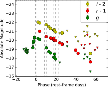
Figure 2. Light curves of iPTF 16asu in g, r, and i filters. As indicated in the legend, the r and i band data have been offset for clarity. Triangles denote nondetections. Dashed lines indicate times of spectroscopic observations.
Download figure:
Standard image High-resolution imageTable 1. Log of iPTF 16asu Photometric Observations
| Observation Date | Phasea | Filter | Magnitudeb | Telescope |
|---|---|---|---|---|
| (MJD) | (rest-frame days) | (AB) | ||
| 57508.32 | −12.50 | g | >20.61 | P48 |
| 57510.27 | −10.87 | g | >20.89 | P48 |
| 57510.30 | −10.84 | g | >20.80 | P48 |
| 57510.33 | −10.82 | g | >20.91 | P48 |
| 57511.26 | −10.03 | g | >20.78 | P48 |
| 57511.29 | −10.00 | g | >20.72 | P48 |
| 57511.32 | −9.98 | g | >20.53 | P48 |
| 57512.26 | −9.18 | g | >21.05 | P48 |
| 57512.29 | −9.16 | g | >20.82 | P48 |
| 57512.32 | −9.14 | g | >21.09 | P48 |
| 57513.25 | −8.35 | g | >20.96 | P48 |
| 57513.28 | −8.33 | g | >20.96 | P48 |
| 57513.31 | −8.30 | g | >20.72 | P48 |
| 57519.26 | −3.29 | g | 20.43 ± 0.13 | P48 |
| 57519.29 | −3.27 | g | >20.29 | P48 |
| 57519.32 | −3.24 | g | >20.01 | P48 |
| 57520.25 | −2.46 | g | 19.80 ± 0.12 | P48 |
| 57520.28 | −2.43 | g | 19.69 ± 0.08 | P48 |
| 57521.26 | −1.61 | g | 19.34 ± 0.09 | P48 |
| 57521.29 | −1.58 | g | 19.25 ± 0.09 | P48 |
| 57521.32 | −1.56 | g | 19.28 ± 0.09 | P48 |
| 57525.40 | 1.88 | g | 19.38 ± 0.09 | P60 |
| 57527.34 | 3.51 | g | 19.51 ± 0.07 | P60 |
| 57535.33 | 10.24 | g | 20.43 ± 0.09 | P60 |
| 57538.34 | 12.78 | g | 20.87 ± 0.05 | P60 |
| 57540.30 | 14.42 | g | 21.01 ± 0.07 | P60 |
| 57544.21 | 17.72 | g | 21.49 ± 0.08 | P60 |
| 57545.25 | 18.60 | g | 21.48 ± 0.11 | P60 |
| 57545.26 | 18.61 | g | 21.14 ± 0.09 | P60 |
| 57546.31 | 19.49 | g | 21.69 ± 0.13 | P60 |
| 57551.35 | 23.73 | g | >22.09 | P60 |
| 57560.26 | 31.24 | g | >20.29 | P60 |
| 57580.20 | 48.03 | g | >21.69 | P60 |
| 57581.23 | 48.90 | g | >21.19 | P60 |
| 57584.24 | 51.43 | g | >21.49 | P60 |
| 57587.18 | 53.91 | g | >21.69 | P60 |
| 57587.88 | 54.50 | g | >23.09 | TNG |
| 57527.33 | 3.51 | r | 19.60 ± 0.09 | P60 |
| 57535.32 | 10.23 | r | 20.19 ± 0.07 | P60 |
| 57540.27 | 14.40 | r | 20.34 ± 0.04 | P60 |
| 57541.18 | 15.17 | r | 20.40 ± 0.12 | P60 |
| 57541.18 | 15.17 | r | 20.36 ± 0.07 | P60 |
| 57544.19 | 17.70 | r | 20.55 ± 0.05 | P60 |
| 57544.25 | 17.75 | r | 20.55 ± 0.04 | P60 |
| 57544.26 | 17.76 | r | 20.37 ± 0.03 | P60 |
| 57545.23 | 18.58 | r | 20.65 ± 0.07 | P60 |
| 57545.23 | 18.58 | r | 20.61 ± 0.09 | P60 |
| 57546.29 | 19.47 | r | 20.64 ± 0.05 | P60 |
| 57551.32 | 23.71 | r | 20.89 ± 0.13 | P60 |
| 57554.24 | 26.17 | r | 21.09 ± 0.15 | P60 |
| 57554.25 | 26.17 | r | 21.00 ± 0.12 | P60 |
| 57560.24 | 31.22 | r | >20.83 | P60 |
| 57570.22 | 39.62 | r | 21.73 ± 0.20 | P60 |
| 57573.21 | 42.14 | r | 22.06 ± 0.14 | P60 |
| 57577.25 | 45.55 | r | >21.13 | P60 |
| 57580.19 | 48.02 | r | >21.53 | P60 |
| 57581.22 | 48.89 | r | >21.13 | P60 |
| 57584.23 | 51.42 | r | >20.03 | P60 |
| 57587.17 | 53.90 | r | >21.03 | P60 |
| 57587.90 | 54.52 | r | 23.01 ± 0.15 | TNG |
| 57593.21 | 58.99 | r | >21.73 | P60 |
| 57596.21 | 61.51 | r | >21.43 | P60 |
| 57525.40 | 1.88 | i | 19.57 ± 0.14 | P60 |
| 57527.33 | 3.51 | i | 19.66 ± 0.07 | P60 |
| 57535.33 | 10.24 | i | 19.87 ± 0.05 | P60 |
| 57538.33 | 12.77 | i | 20.09 ± 0.05 | P60 |
| 57540.28 | 14.41 | i | 20.29 ± 0.06 | P60 |
| 57544.20 | 17.71 | i | 20.46 ± 0.05 | P60 |
| 57544.21 | 17.72 | i | 20.43 ± 0.05 | P60 |
| 57544.26 | 17.77 | i | 20.43 ± 0.06 | P60 |
| 57545.24 | 18.59 | i | 20.48 ± 0.11 | P60 |
| 57545.25 | 18.59 | i | 20.46 ± 0.10 | P60 |
| 57546.29 | 19.48 | i | 20.68 ± 0.08 | P60 |
| 57551.33 | 23.72 | i | >20.84 | P60 |
| 57554.25 | 26.18 | i | 20.82 ± 0.16 | P60 |
| 57554.26 | 26.19 | i | 20.73 ± 0.12 | P60 |
| 57560.25 | 31.23 | i | >20.55 | P60 |
| 57570.23 | 39.63 | i | >21.25 | P60 |
| 57573.21 | 42.15 | i | >21.75 | P60 |
| 57580.20 | 48.03 | i | >20.64 | P60 |
| 57581.22 | 48.89 | i | >21.14 | P60 |
| 57584.23 | 51.43 | i | >20.05 | P60 |
| 57584.26 | 51.45 | i | >20.75 | P60 |
| 57587.17 | 53.90 | i | >21.25 | P60 |
| 57587.89 | 54.51 | i | 23.07 ± 0.16 | TNG |
| 57593.22 | 58.99 | i | >20.95 | P60 |
| 57596.21 | 61.51 | i | >21.14 | P60 |
| 57527.29 | 3.47 | V | >19.48 | Swift |
| 57527.29 | 3.47 | B | 19.45 ± 0.2 | Swift |
| 57527.29 | 3.47 | u | 19.6 ± 0.14 | Swift |
| 57527.29 | 3.47 | UVW1 | 20.52 ± 0.14 | Swift |
| 57527.29 | 3.47 | UVW2 | 21.8 ± 0.19 | Swift |
| 57527.29 | 3.47 | UVM2 | 21.27 ± 0.14 | Swift |
| 57534.33 | 9.4 | V | >18.95 | Swift |
| 57534.33 | 9.4 | B | >19.61 | Swift |
| 57534.33 | 9.4 | u | >20.37 | Swift |
| 57534.33 | 9.4 | UVW1 | >21.46 | Swift |
| 57534.33 | 9.4 | UVW2 | >22.46 | Swift |
| 57534.33 | 9.4 | UVM2 | >22.48 | Swift |
| 57541.19 | 9.4 | V | >18.96 | Swift |
| 57541.19 | 9.4 | B | >19.86 | Swift |
| 57541.19 | 9.4 | u | >20.68 | Swift |
| 57541.19 | 9.4 | UVW1 | >21.78 | Swift |
| 57541.19 | 9.4 | UVW2 | >22.60 | Swift |
| 57541.19 | 9.4 | UVM2 | >22.56 | Swift |
Notes.
aPhase is in rest-frame days relative to bolometric maximum light. bCorrected for Galactic extinction.Only a portion of this table is shown here to demonstrate its form and content. A machine-readable version of the full table is available.
2.3. Spectroscopy
We obtained a sequence of eight low-resolution spectra for iPTF 16asu using the DBSP on P200, the Andalucia Faint Object Spectrograph and Camera (ALFOSC) on the 2.56 m Nordic Optical Telescope (NOT), the Device Optimized for the Low Resolution (DOLORES) on TNG, the Low-resolution Imaging Spectrometer (LRIS; Oke et al. 1995) on Keck I, and the DEIMOS on the 10 m Keck II Telescope. The times of the spectra are marked as dashed lines in Figure 2, and details of the spectroscopic observations are given in Table 2. Spectra were reduced using standard procedures using IRAF18 and IDL, including wavelength calibration using arc lamps and flux calibration using standard stars. The spectroscopic sequences for iPTF 16asu is shown in Figure 3, and the spectroscopic properties are analyzed and discussed in Section 4. All spectra will be made available in the Weizmann Interactive Supernova Data Repository (Yaron & Gal-Yam 2012).
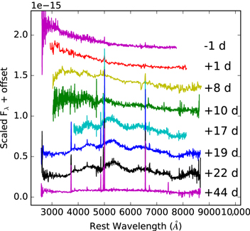
Figure 3. Sequence of observed spectra for iPTF 16asu. Phase in rest-frame days relative to g band maximum is given to the right of each spectrum. The first two spectra show a featureless blue continuum, with broad SN features starting to be visible eight days after maximum. By day 17, the spectrum has developed into that of an SN Ic-BL. Our last spectrum, taken 44 days after peak, is dominated by galaxy light. Galaxy narrow emission lines have not been removed. Spectra have been binned and arbitrarily scaled for display purposes. See Section 4 for details.
Download figure:
Standard image High-resolution imageTable 2. Log of iPTF 16asu Spectroscopic Observations
| Observation Date | Phasea | Instrument | Grating | Filter | Wavelength | Resolution | Exp. Time | Airmass |
|---|---|---|---|---|---|---|---|---|
| (rest-frame days) | (Å) | (Å) | (s) | |||||
| 2016 May 14.30 | −0.73 | P200+DBSP | 600/4000 | None | 3101–9199 | 1.30 | 600 | 1.21 |
| 2016 May 16.06 | +0.75 | NOT+ALFOSC | GRISM 4 | None | 3478–9662 | 3.35 | 2400 | 1.35 |
| 2016 May 24.97 | +8.25 | TNG+DOLORES | LR-B + LR-R | None | 3315–10330 | 2.65 | 2100 | 1.09 |
| 2016 May 27.36 | +10.27 | P200+DBSP | 600/4000 | None | 3600–10237 | 1.30 | 1800 | 1.69 |
| 2016 Jun 04.39 | +17.03 | Keck 2+DEIMOS | 600ZD | GG455 | 4550–9649 | 0.65 | 1000 | 1.29 |
| 2016 Jun 07.36 | +19.53 | Keck 1+LRIS | 400/3400, 400/8500 | None | 3072–10285 | 1.55 | 950 | 1.17 |
| 2016 Jun 10.42 | +22.11 | Keck 1+LRIS | 400/3400, 400/8500 | None | 3101–10290 | 1.55 | 980 | 1.71 |
| 2016 Jul 06.30 | +43.92 | Keck 1+LRIS | 400/3400, 400/8500 | None | 3067–10289 | 1.55 | 2400 | 1.30 |
| 2017 Apr 29.39 | +294.04 | Keck 1+LRIS | 400/3400, 400/8500 | None | 3063–10318 | 1.55 | 2400 | 1.02 |
Note.
aPhase is in rest-frame days relative to the bolometric maximum light (MJD 57523.25).Download table as: ASCIITypeset image
2.4. Radio Observations
We observed the field of iPTF 16asu with the Karl G. Jansky Very Large Array (VLA) on two epochs (Program VLA/16B-043; PI: A. Corsi). The first observation was carried out starting on 2016 June 13, 01:18:22 UT (MJD 57552), with the VLA in its B configuration. The second observation was carried out with the VLA in its A configuration, starting on 2017 January 10, 09:43:06 UT (MJD 57763). Both these observations were carried out in the C band (nominal central frequency of ≈5 GHz), using the 8 bit configuration and 2 GHz nominal bandwidth. On both epochs we used 3C286 as a bandpass and flux density calibrator and J1300 + 1417 as a phase calibrator. The total observing time was about 1 hr (including calibration and overhead) per epoch.
VLA data were calibrated using the automated VLA calibration pipeline in CASA (McMullin et al. 2007). After visual inspection, additional flags were applied when needed. Images of the fields were produced using the CLEAN task (Högbom 1974).
We searched for a radio counterpart to iPTF 16asu within a 2'' radius circle centered on the iPTF position of iPTF 16asu. No radio source was detected within this region down to a 3σ limit of  at 6.2 GHz for both epochs.
2.5. UV and X-Ray Observations
At the time of the first spectrum, iPTF 16asu resembled a very young SLSN, with its already high luminosity and blue spectrum indicating a high temperature. We therefore triggered our Swift program for SLSNe (GI-1215281, PI: R. Lunnan), and three epochs of Swift UVOT (Roming et al. 2005) and XRT (Burrows et al. 2005) data were obtained at phases corresponding to 7.4, 13.4, and 19.2 days after explosion (see Section 3.1 for the calculation of the explosion date).
We reduced the Swift data using the HEASoft package provided by NASA.19 UVOT photometry was performed using the task UVOTsource with an aperture of 5''. iPTF 16asu was detected in all filters except the V band in the first observation and undetected in all UVOT filters in the subsequent two epochs, due to the rapid fading of the SN. All UVOT photometry is listed in Table 1.
The XRT data were reduced with the Ximage software from the HEASoft package. No X-ray source was detected at the position of iPTF 16asu in either epoch. The  upper limits correspond to
  counts s−1,
  counts s−1, and
  counts s−1, respectively. Using WebPIMMS20
and assuming a Galactic nH of
counts s−1, respectively. Using WebPIMMS20
and assuming a Galactic nH of  , we find that
  counts s−1 corresponds to
  (unabsorbed; 0.3–10 keV), assuming a power-law model with an index of 2. At a redshift of z = 0.1874, our X-ray count limits translates to flux limits of
  ,
,  , and
, and  , respectively.
2.6. Search for Associated GRBs
We searched the Gamma-Ray Coordinates Network archives for any announced GRBs consistent with the location and best-fit explosion time of iPTF 16asu (Section 3.1). No announced GRB was consistent with the location and time of iPTF 16asu or when extending the search to include bursts detected between the last iPTF nondetection and the first detection of iPTF 16asu. However, our analysis of the Konus-Wind data (KW; Aptekar et al. 1995) reveals that a weak burst was detected by KW in the waiting mode (with a time resolution of 2.944 s) on 2016 May 10.41, which is consistent with our best-fit explosion time of 2016 May 10.53 ± 0.17 days (see Section 3.1). The burst was observed by the KW S2 detector pointing the northern ecliptic hemisphere (nothing was seen in the opposite S1 detector), which is also consistent with the position of iPTF 16asu, but the burst source position cannot be constrained more precisely from the KW data.
The burst emission was significant in the two softest KW energy bands: G1 (20–80 keV,  ) and G2 (80–300 keV,
  ). The burst light curve shows a single emission episode with a duration of 126 s (T50 = 56 ± 11 s and T90 = 100 ± 11 s, both measured in the 20–300 keV energy band). Fitting the KW tree-channel time-integrated spectrum (measured from T0 to T0+126.592 s) by a simple power law yields the photon index of
  ,
,  . From this fit, the burst had an energy fluence of
  and a 2.944 s peak energy flux, measured from T0 + 73.6 s, of
  (both in the 20–1200 keV energy range). At the distance of iPTF 16asu, this fluence would correspond to an equivalent isotropic energy
  of
of  . The fit with a power law with an exponential cutoff model yields only an upper limit on spectrum peak energy:
  .
.
During the KW burst, Swift was in the South Atlantic Anomaly and the position of iPTF 16asu was Earth-occulted. However, the position of iPTF 16asu was not occulted for Fermi (and six GBM detectors had incident angles of less than 60°). We analyzed the Fermi-GBM continuous data and found no emission in the 30–300 keV band coincident with the KW burst. Given that the background of Fermi-GBM is considerably lower than KW, this implies that the KW burst came from a source Earth-occulted to Fermi and therefore is not related to iPTF 16asu.
We also searched for a possible GRB in the INTEGRAL-SPI-ACS (SPI-ACS; von Kienlin et al. 2003) data covering the 75–8000 keV range and found no candidate event down to the 3 sigma level. Since KW and SPI-ACS were observing the whole sky during the interval of interest, upper limits on gamma-ray flux can be obtained. For the whole interval (excluding the KW burst), assuming a typical long GRB spectrum (the band function with  ,
,  , and
, and  ), the corresponding KW and SPI-ACS limiting peak fluxes estimates are
  , both in the 10 keV–10 MeV band at 3–10 s time scales.
We conclude therefore that there is no statistically significant evidence for an SN-associated GRB down to the threshold of  . The associated isotropic peak luminosity limit is
  and the total energy is
  (both calculated in the 10 keV–10 MeV energy range). Hence from these limits an accompanying low-luminosity GRB, like GRB 980425 (
 ,
,  Galama et al. 1998b), cannot be excluded. We return to discuss possible GRB models for iPTF 16asu in Section 6.3.
3. Light Curve Analysis
3.1. Rise Time and Peak Luminosity
The light curves of iPTF 16asu are shown in Figure 2. The rise and peak are only sampled in the g band, so we fit a second-order polynomial to the g band light curve near peak brightness to determine a best-fit explosion date, time of peak, and peak luminosity. The fit is shown in Figure 4, and the explosion and best-fit peak dates are MJD 57518.53 ± 0.17 and MJD 57523.25 ± 0.14, respectively. Corresponding calendar dates are 2016 May 10.53 and 2016 May 15.25. Thus, the rise time (time of peak—time of explosion) is 3.97 ± 0.19 days in the rest frame. The last optical upper limit prior to the first detection was MJD 57513.31, setting an upper limit to the rise time of 9.94 days.

Figure 4. Early g band light curve of iPTF 16asu, showing the rise of the light curve to peak. Red triangles denote g band nondetections. The second-order polynomial best-fit line (blue) results in a calculated rise time of 3.97 ± 0.19 days. The equation of line of best fit is  , where x is the phase in days and y is the flux (Fλ) in arbitrary units.
Download figure:
Standard image High-resolution imageUsing our series of spectra, we calculate K-corrections from the observed filters at z = 0.187 to the rest-frame filters, listed in Table 3. At this redshift the observed gri corresponds most closely to the rest-frame BVr, and the wavelength coverage of our spectra allows us to also calculate K-corrections to the u, g, and i filters. Applying this, we find that the time of peak corresponds to a peak absolute magnitude of  mag (AB).
Table 3. K-corrections Derived from Spectra
| Phase |

|

|

|

|

|

|

|

|
|---|---|---|---|---|---|---|---|---|
| (rest-frame days) | (mag) | (mag) | (mag) | (mag) | (mag) | (mag) | (mag) | (mag) |
| −0.73 | −0.368 | −0.041 | −0.270 | −0.194 | ⋯ | −0.173 | −0.192 | −0.269 |
| +0.75 | −0.357 | −0.062 | −0.260 | −0.215 | ⋯ | −0.164 | −0.177 | −0.258 |
| +8.25 | −0.136 | −0.286 | 0.056 | −0.372 | −0.285 | −0.206 | −0.078 | −0.175 |
| +10.27 | −0.107 | −0.280 | 0.062 | −0.438 | −0.325 | −0.204 | −0.079 | −0.158 |
| +17.03 | −0.109 | ⋯ | ⋯ | ⋯ | ⋯ | −0.199 | ⋯ | −0.121 |
| +19.53 | −0.043 | −0.467 | 0.410 | −0.688 | −0.255 | −0.195 | 0.102 | −0.112 |
| +22.11 | −0.050 | −0.487 | 0.422 | −0.768 | −0.214 | −0.187 | 0.127 | −0.110 |
Notes.
aK-correction is defined as in Hogg et al. (2002), so that for filters Q and R, .
bPhase is in rest-frame days relative to the bolometric maximum light (MJD 57523.25).
.
bPhase is in rest-frame days relative to the bolometric maximum light (MJD 57523.25).
Download table as: ASCIITypeset image
3.2. Light Curve Comparisons
iPTF 16asu inhabits an unusual location in rise time versus luminosity parameter space (see Figure 1). In this section, we compare its light curve in more detail to objects in the literature that have been noted for their fast timescales and/or high luminosities. Unfortunately, K-corrections are not available for the majority of our comparison objects due to a lack of spectroscopic coverage. For the purposes of comparison, we corrected iPTF 16asu and all comparison objects for redshift using the following equations:

We then chose filters with rest wavelengths as closely corresponding to those of iPTF16asu as possible in order to facilitate comparison. Comparing the approximation used in Equation (2) to the actual K-corrections calculated for iPTF 16asu (Table 3), we expect this approximation to introduce errors on the order of 0.1 mag. Figure 5 shows comparisons to the g band (left) and r band (right) light curves.
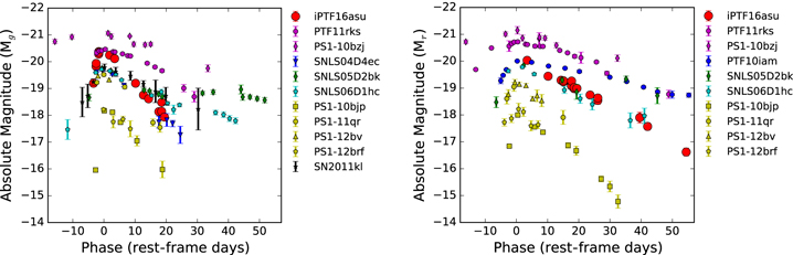
Figure 5. g-band (left) and r-band (right) light curves of iPTF 16asu (red) compared to other luminous and/or rapidly evolving transients from the literature. Filters have been chosen to correspond to approximately the same rest wavelengths. SLSNe from Inserra et al. (2013) and Lunnan et al. (2013) are shown in magenta; Arcavi et al. (2016) objects are shown in blue, cyan, and green; Drout et al. (2014) objects are shown in yellow; and SN 2011kl/GRB 111209A (Greiner et al. 2015) objects are shown in black.
Download figure:
Standard image High-resolution image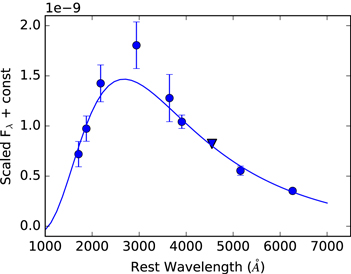
Figure 6. Blackbody fit of the Swift/UVOT and optical data, at phase +3 days. The triangle denotes a nondetection in the V band. The best-fit estimates of the temperature and radius from the fit are T = 10,800 ± 250 K and  cm.
cm.
Download figure:
Standard image High-resolution imageFirst we compare against the light curves of SNe noted for both their high luminosities and their rapid timescales. These include SN 2011kl (Greiner et al. 2015), an SN associated with the ultralong gamma-ray burst GRB 111209A (plotted in black), and PTF 10iam (blue), SNLS04D4ec (blue), SNLS05D2bk (green), and SNLS06D1hc (cyan) from Arcavi et al. (2016). In the g band as seen in Figure 5 (left), iPTF 16asu reaches a higher peak luminosity than these transients by over half a magnitude. Measuring from the rest-frame phase at  to
to  , iPTF 16asu's timescale is about two times shorter with
  days. iPTF 16asu displays both a steeper rise and steeper decay than the Arcavi et al. (2016) objects and SN 2011kl in the g band. However, iPTF 16asu resembles these objects more closely in the r band, shown in Figure 5 (right). The peak r band magnitude of iPTF 16asu is approximately the same as PTF 10iam, SNLS05D2bk, and SNLS06D1hc and the slope of decay runs nearly parallel to that of SNLS06D1hc. Although we have no data on the rise in the r band, iPTF 16asu has a peak magnitude similar to that of to the Arcavi et al. (2016) objects and decays on the same timescale as SNLS06D1hc.
Next we compared the light curve to PS1-10bjp, PS1-11qr, PS1-12bv, and PS1-12brf, a sample of rapidly evolving transients from the Pan-STARRS1 Medium Deep Survey (Drout et al. 2014). The objects shown are the four most luminous objects from the "gold" sample and are plotted in yellow in Figure 5. They have rise times and decay slopes similar to those of iPTF 16asu but are much fainter. In the g band, PS1-11qr and PS1-12bv are the brightest of the Pan-STARRS1 objects, reaching a peak magnitude of about −19.5 mag; thus iPTF 16asu is a magnitude brighter at peak. As seen in Figure 5, the shape of iPTF 16asu's light curve is quite similar to that of PS1-10bjp and PS1-11qr. Early in the decay of iPTF 16asu, the slope is nearly parallel to that of PS1-10bjp; however, at late times PS1-10bjp decays more sharply than iPTF 16asu. Comparing these objects to the r band data is less instructive because iPTF 16asu's rise was not captured in the r band and most of the Pan-STARRS1 objects do not have late-time data.
Finally we compared iPTF 16asu to the SLSNe PTF11rks (Inserra et al. 2013) and PS1-10bzj (Lunnan et al. 2013), which are both on the lower-luminosity end of SLSNe. In the g band, iPTF 16asu reaches about the same peak absolute magnitude as PTF11rks. In the r band iPTF 16asu's peak luminosity is about 0.5 mag dimmer than that of PTF11rks. However, the SLSNe have timescales several times longer than that of iPTF 16asu, as seen by the much broader peaks. Thus, while iPTF 16asu reaches luminosities similar to those of some SLSNe, it evolves on a very different timescale. iPTF 16asu stands out as a unique and surprising event, even amongst similar transients from the literature.
3.3. Blackbody Fits
We fit a blackbody to all epochs where we have observations in at least three filters, using Scipy least-squares optimization routines (Jones et al. 2001) as well as to our two earliest spectra. Only the day with Swift/UVOT detections (+3 days past peak) has data in more than three filters. The fit to the Swift photometry is shown in Figure 6. From this fit we obtain T = 10,800 ± 250 K and R = (2.6 ± 0.2) × 1015 cm. This corresponds to a total blackbody luminosity of  erg s−1.

Figure 7. Blackbody temperature (left) and radius (right) as a function of time. We fit a blackbody to all epochs with photometry in at least three filters as well as to the earliest two spectra. The slope of the radius over time gives an estimated expansion velocity of 35,400 ± 5350 km s−1. Open circles indicate points for which the covariance matrix would not converge to give error bars.
Download figure:
Standard image High-resolution imageFigure 7 shows the resulting derived temperatures and radii at all epochs. The overall trends show a cooling blackbody temperature and an increasing radius. In fitting a straight line to the blackbody radii, we get a best-fit slope of 34,500 ± 5400 km s−1, indicating high average velocities.

Figure 8. Left: Pseudobolometric light curve of iPTF 16asu. Luminosities obtained from data using the trapezoidal integration method. Right: Fit of the decline of iPTF 16asu's light curve to a power law and an exponential. The power law (dashed blue) has a best-fit of  and the exponential (solid green) decays are on a timescale of
  days. The light curve decline is well fit by an exponential.
Download figure:
Standard image High-resolution image3.4. Bolometric Light Curve
We construct a pseudobolometric light curve for iPTF 16asu by summing the observed flux on days where we have observations in at least three filters. We integrate over the observed spectral energy distribution using trapezoidal integration, interpolating to the edges of the observed bands. Since this only accounts for the observed flux, it constitutes a strict lower limit on the true bolometric luminosity.
Pre-peak photometry is only available in the g band so we approximate the rise of the pseudobolometric light curve by assuming a constant ratio of g band flux to total flux, i.e., a constant bolometric correction. This assumption is equivalent to assuming that the temperature on the rise is constant and equal to the temperature measured from the earliest multiband data. Similarly, for the late-time observations with data only in the r band we estimate the total flux by using the same bolometric correction as from the latest date with data in  filters.
We caution that in constructing a pseudobolometric light curve from optical data only, we are implicitly assuming that the ratio of optical to bolometric flux is approximately constant over the time period of interest. In particular, at late times as the effective temperature falls we would expect the near-IR (NIR) fraction of the bolometric luminosity to increase, which is unconstrained from observations, so assuming a constant bolometric correction is likely an underestimate. Unfortunately, NIR data are also not available for other fast-evolving SNe so we cannot use them as a basis for comparison. However, given that iPTF 16asu resembles a normal SN Ic-BL–like SN 1998bw from ∼20 days past explosion onward (Sections 4 and 6.1), we expect its late-time evolution of the optical-to-bolometric flux ratio to resemble normal SNe Ic-BL. Comparing to the light curve samples analyzed in Lyman et al. (2014), we estimate that this adds an uncertainty on the level of 10%–20% at late times.
Figure 8 (left) shows the resulting pseudobolometric light curve. Using trapezoidal integration over time we calculate an estimated total radiated energy of  erg and a peak luminosity of
  erg s−1.
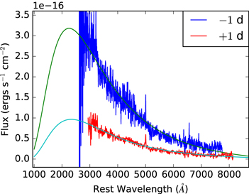
Figure 9. Blackbody fit of the two earliest spectra. The corresponding temperature and radius at phase −1 day are T = 10828 ± 322 K and  cm. The corresponding temperature and radius at phase +1 day are T = 10,466 ± 232 K and
  cm.
cm.
Download figure:
Standard image High-resolution imageThe shape of the decline of the bolometric light curve sheds light on what physical processes may be powering this event. Figure 8 (right) shows the best-fit power law and exponential fits to the post-peak light curve. Clearly the decline of the light curve does not follow a power law; however, it fits an exponential well. The power law has a best-fit decay of  and the exponential decays are on a timescale of
  days. The power-law decay parameter is similar to those found for the objects in Arcavi et al. (2016). Also similar, two of the four Arcavi et al. (2016) objects are better fit by an exponential. The implications of these results are discussed in Section 6.
4. Spectroscopic Properties
4.1. Spectroscopic Evolution and Comparisons
We obtained eight spectra of iPTF 16asu between 2016 May 14 and 2016 Jul 6. The spectra are shown in Figure 3. In this section, we look at the spectroscopic evolution in more detail and compare the spectroscopic properties of iPTF 16asu to similar objects from the literature.
The first two spectra, taken within a day before and after peak, show a featureless blue continuum with no discernible broad features. The spectrum is well fit by a blackbody, as shown in Figure 9. Such spectra dominated by blue continua have also been observed at early phases in other SNe, typically while the luminosity is powered by the cooling of the stellar envelope following shock breakout (see, e.g., SN 1993J; Woosley et al. 1994; Matheson et al. 2000). Interestingly, the rapidly evolving SNe from Pan-STARRS1 (Drout et al. 2014) also showed featureless blue continua. Figure 10 shows a comparison of PS1-12bv at peak compared to iPTF 16asu at peak. Unfortunately, comparison at late times is not possible as there is no further follow-up spectroscopy on the Pan-STARRS1 events. Based on the limited spectroscopic data available we cannot rule out that they were caused by the same phenomenon as iPTF 16asu.
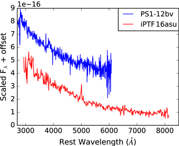
Figure 10. Spectrum of PS1-12bv (Drout et al. 2014) at +7 days after explosion compared to iPTF 16asu at +5 days after explosion. iPTF 16asu spectrum from NOT. Host galaxy narrow emission lines have not been removed—note that the feature at ∼5000 Å in the iPTF 16asu spectrum is a narrow [O iii]  4959,5007 emission from the host galaxy that appears broadened here due to binning.
Download figure:
Standard image High-resolution imageThe next two spectra, taken at phases 8 and 10 days past maximum, still show an underlying blue continuum but with broad features emerging. Such an evolution is reminiscent of GRB SNe. To illustrate this we show a comparison to SN 2006aj/GRB 060218 (Modjaz et al. 2006) in Figure 11. SN 2006aj is of particular interest here because it is one of the few GRB SNe that would not be ruled out by our radio and X-ray limits. We discuss GRB models for iPTF 16asu in detail in Section 6.3.

Figure 11. Spectrum of SN 2006aj (Modjaz et al. 2006) at +6 days after explosion compared to iPTF 16asu at +12 days after explosion. iPTF 16asu spectrum from TNG. Host galaxy narrow emission lines have not been removed.
Download figure:
Standard image High-resolution imageThe three spectra taken at phases +17, +19, and +22 days post maximum are dominated by distinct broad-line features, leading us to classify iPTF 16asu as an SN Ic-BL. Figure 12 shows a comparison of iPTF 16asu at +23 days after explosion (+19 days past peak) to SN 1998bw at +18 days after explosion, and features commonly identified in SNe Ic-BL are marked. Interestingly, the spectra of these events look very similar at roughly the same time after explosion, suggesting that iPTF 16asu may have a normal-timescale SN component hidden underneath the luminous and rapidly evolving peak.
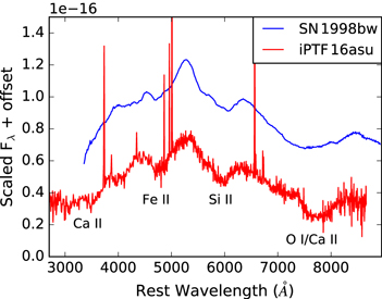
Figure 12. Spectrum of SN 1998bw (Patat et al. 2001) at +18 days after explosion compared with iPTF 16asu at +23 days after explosion. Features commonly identified in SNe Ic-BL are marked. iPTF 16asu spectrum from Keck 1+LRIS. Host galaxy narrow emission lines have not been removed.
Download figure:
Standard image High-resolution imageIt is also worth noting that the spectroscopic evolution of iPTF 16asu is different from the few objects in Drout et al. (2014) and Arcavi et al. (2016) with spectra at later phases: PS1-12bb showed a featureless continuum at phase +33 days, while PTF 10iam showed broad Hα emission at phase +28 days. This spectroscopic diversity suggests that there are likely multiple physical mechanisms giving rise to light curves in this part of the transient phase space.
Our final spectrum, taken at phase +44 days past peak, is dominated by host galaxy light. We discuss the host galaxy properties in Section 5.
4.2. Velocities
Measuring velocities from SNe Ic-BL spectra is challenging since the lines are often blended due to the high velocities. In addition, different lines can give different velocities because these elements are formed and found at different radii in the expanding ejected material. For iPTF 16asu we chose the strongest lines: the Si ii  Å line and the Fe ii
  Å line.
In the case of the Si ii  Å line we fit a parabola to find the minimum of the broad absorption feature. The corresponding wavelength is then used to determine velocities using the relativistic Doppler shift. The measured velocities are listed in Table 4.
Table 4. Spectral Line Velocities of iPTF 16asu
| Observation Date | Phasea | Fe ii Velocity | Fe ii Broadening | Si ii Velocity |
|---|---|---|---|---|
| (rest-frame days) | (1000 km s−1) | (1000 km s−1) | (1000 km s−1) | |
| 2016 May 24.97 | +8.25 |

|

|
|
| 2016 May 27.36 | +10.27 |

|

|
23.3 |
| 2016 Jun 04.39 | +17.03 |

|

|
19.8 |
| 2016 Jun 07.36 | +19.53 |

|

|
19.2 |
| 2016 Jun 10.42 | +22.11 |

|

|
16.8 |
Note.
aPhase is in rest-frame days relative to the bolometric maximum light (MJD 57523.25).Download table as: ASCIITypeset image
In the case of the Fe ii  Å line, similar to other SNe Ic-BL, this line is blended with the neighboring Fe ii λ4924 and Fe ii λ5018 lines. Thus we cannot simply fit the minimum of this feature to derive velocities. Instead we use the convolution method developed by Modjaz et al. (2016) and Liu et al. (2016) to extract velocities from the Fe ii
  Å line. The measured velocities are listed in Table 4. Figure 13 shows the Fe ii velocities from iPTF 16asu compared to the sample of SNe Ic and Ic-BL from Modjaz et al. (2016), with velocities derived using the same method (and code). The Fe ii velocities we measure for iPTF 16asu are high compared to the objects in this sample, closest to the Fe ii velocities of SNe Ic-BL associated with GRBs. We note that phase in this figure is measured with respect to maximum light—if iPTF 16asu has a normal SN component hidden underneath the blue luminous peak, then the SN maximum will be later and iPTF 16asu will move left in this plot, but the basic conclusion that the velocities are comparable to SNe Ic-BL with associated GRBs will be unchanged.

Figure 13. Velocity evolution of iPTF 16asu, measured from the Fe ii  Å line (red points), compared against literature data of SNe Ic (green diamonds), SNe Ic-BL (blue squares), and SNe Ic-BL (yellow triangles) associated with GRBs. Data from Modjaz et al. (2016).
Download figure:
Standard image High-resolution image5. Host Galaxy
The host galaxy of iPTF 16asu is detected in both the PTF templates and the SDSS images. The observed SDSS model magnitudes are  mag,
mag,  mag,
mag,  mag,
mag,  mag, and
  mag. At a redshift of z = 0.1874 this makes the host a dwarf galaxy with an absolute magnitude of
  . We use the FAST code (Kriek et al. 2009) to fit a galaxy model to the observed photometry using a Maraston (2005) stellar population synthesis model, assuming a Salpeter initial mass function and an exponential star formation history. The metallicity and extinction are constrained by our spectroscopic data, so we use the extinction derived from the Balmer decrement and a metallicity of
  , which is the closest model grid value to our derived metallicity. With these assumptions, we find a best-fit stellar mass of
  and a best-fit stellar population age of
  .
.
We obtained a host galaxy spectrum nearly a year after explosion, shown in Figure 14. We scale this galaxy spectrum to the SDSS photometry to account for slit losses, and measure the fluxes of the (unresolved) lines by fitting Gaussian profiles. The measured emission line fluxes are listed in Table 5.

Figure 14. Spectrum of the host galaxy of iPTF 16asu, taken with Keck 1+LRIS at ∼300 days after the SN explosion. Strong galaxy emission lines are marked.
Download figure:
Standard image High-resolution imageTable 5. Host Galaxy Emission Line Fluxes
| Line | Flux |
|---|---|
( ) ) |
|
| [O ii] 3727 | 3.50 ± 0.10 |
| [Ne iii] 3869 | 0.62 ± 0.08 |
| Hγ 4341 | 0.56 ± 0.07 |
| Hβ 4861 | 1.41 ± 0.08 |
| [O iii] 4959 | 1.91 ± 0.12 |
| [O iii] 5007 | 5.72 ± 0.09 |
| Hα 6563 | 5.01 ± 0.09 |
| [N ii] 6583 | 0.24 ± 0.10 |
| [S ii] 6717 | 0.66 ± 0.13 |
| [S ii] 6731 | 0.41 ± 0.14 |
Download table as: ASCIITypeset image
We use the Balmer decrement to calculate the host galaxy extinction, assuming Case B recombination (Osterbrock 1989). We measure a  ratio of 3.5 ± 0.2, translating to a host extinction of
  , assuming a standard Milky Way extinction curve with RV = 3.1 (Cardelli et al. 1989). Using the extinction-corrected
  flux, we measure a star formation rate of 0.7 M⊙
  (Kennicutt 1998). Given the stellar mass derived from the photometry, this corresponds to a specific star formation rate of
  .
.
We use pyMCZ (Bianco et al. 2016) to calculate the galaxy oxygen metallicity from the [O iii], [O ii], [N ii], Hα, and Hβ lines. pyMCZ is a Python-based implementation of up to 15 metallicity calibrators, updating the code given in Kewley & Dopita (2002) and Kewley & Ellison (2008) and with better treatment of statistical uncertainty from Monte Carlo sampling. While there is some scatter between the different strong-line metallicity estimators, they generally agree that the host galaxy of iPTF 16asu is low metallicity. For example, we find values of  to be
to be  on the Pettini & Pagel (2004) O3N2 scale,
  on the McGaugh (1991) scale, and
  on the Kobulnicky & Kewley (2004) R23 scale, to name three commonly used indicators. Using a solar oxygen abundance of
  (Asplund et al. 2009), this translates to a metallicity of
  .
.
Taken together, the host galaxy of iPTF 16asu was a low-mass, low-metallicity, star-forming dwarf galaxy. Such an environment is not unusual for SNe Ic-BL, which in general are found in lower-metallicity galaxies than other stripped-envelope SNe; for example, the median metallicity of SN Ic-BL hosts in the compilation of Sanders et al. (2012) was  on the Pettini & Pagel (2004) O3N2 scale. Other rare transients, such as long GRBs and SLSNe, also show a preference for low-metallicity galaxies (e.g., Levesque et al. 2010; Lunnan et al. 2014; Perley et al. 2016). The high specific star formation rate and the strong [O iii]λ5007 Å line (
 , rest-frame) in particular is reminiscent of SLSN host galaxies (Leloudas et al. 2015). Interestingly, the same is not true for the rapidly evolving transients studied in Drout et al. (2014) and Arcavi et al. (2016): for both samples, the host galaxies were generally more massive galaxies near solar metallicity.
6. Model Comparisons
6.1. Nickel Decay
Most SNe Ic/Ic-BL are powered by the release of energetic photons from the radioactive decay of 56Ni into 56Co and finally 56Fe. Since the late-time spectra of iPTF 16asu look very similar to the spectra of other SNe Ic-BL (Section 4), we first consider whether the light curve of iPTF 16asu can be explained purely by the decay of 56Ni.
Using the equations from Section 2 of Lyman et al. (2016), we compare our pseudobolometric light curve from Section 3.4 to the theoretical model for a 56Ni decay–powered light curve in Arnett (1982). The model takes two input parameters: diffusion time and 56Ni mass. The 56Ni mass predominantly affects the luminosity of the light curve, as a larger 56Ni mass would indicate a larger total energy input and the diffusion time controls the timescale over which the energy diffuses out (i.e. width of the peak). Figure 15 shows the bolometric light curve of iPTF 16asu plotted against an Arnett (1982) model with the parameters  M⊙ and
  days, assuming an opacity of
  cm2 g−1. As seen in Figure 15 , the 56Ni decay model does not fit both the sharp peak and the steep decay well, though we caution that the lack of NIR data could mean that our late-time bolometric light curve is systematically underestimated (Section 3.4).

Figure 15. Nickel-powered model fit to the light curve of iPTF 16asu, following Arnett (1982) and Lyman et al. (2016). The red dot-dashed curve shows the model with the parameters  M⊙ and
  days. The dotted gray line shows the model constrained by the last point with the parameters
  M⊙ and
  days. For comparison, the bolometric light curve using
  bands of SN 1998bw (Clocchiatti et al. 2011) is plotted in black. Attempting to fit the sharp luminous light curve with a 56Ni model leads to an unphysical solution in which the derived ejecta mass is lower than the required nickel mass.
Download figure:
Standard image High-resolution imageAn ejecta mass of  M⊙ was calculated using this diffusion time along with an estimate of the kinetic energy. Since our spectra near peak are featureless, and thus we cannot measure a velocity, we used the average velocity (35,000 km s−1) derived from the evolution of the blackbody radii to calculate this kinetic energy. The ejecta mass is notably about 10 times smaller than the amount of 56Ni required to power this light curve, which is unphysical: the 56Ni mass cannot be larger than the total ejecta mass, since it is necessarily part of the ejecta. Thus we rule out spherically symmetric radioactive 56Ni decay as the dominant energy source for iPTF 16asu.
The Arnett model considered above assumes spherical symmetry and a central energy source, i.e., that all the nickel is in the center. Therefore we cannot rule out the possibility of 56Ni-powered models for iPTF 16asu in a highly mixed or strongly asymmetric scenario (e.g., a jet), though we note that assymmetry is not expected to have a large effect on the observed luminosity (Barnes et al. 2017). More sophisticated modeling is outside of the scope of this paper.
Although 56Ni decay alone cannot explain the light curve of iPTF 16asu, it may still contribute. Figure 16 shows iPTF 16asu's light curve compared to other SNe Ic-BL from the literature. The light curve of SN 1998bw in the g and r bands is a good match to that of iPTF 16asu from ∼15 to 40 days, which interestingly also corresponds to the time when their spectra are very similar (Figure 12), suggesting that the light curve of iPTF 16asu could plausibly be dominated by a normal SN component at these times. Their late-time slopes deviate, mainly constrained by our last r band point at 60 days (Figure 16)—however, the decay rates of stripped-envelope SNe are heterogeneous and could be explained by differences in opacity and/or asymmetry, affecting the degree of gamma-ray trapping (Wheeler et al. 2015; Dessart et al. 2017). Fainter SNe Ic-BL such as SN 2006aj and SN 2002ap are below the light curve of iPTF 16asu at all times (Figure 16). Since the light curve shows only a single, smooth peak, any 56Ni decay contribution to the total luminosity must be subdominant to whatever is powering the main peak.
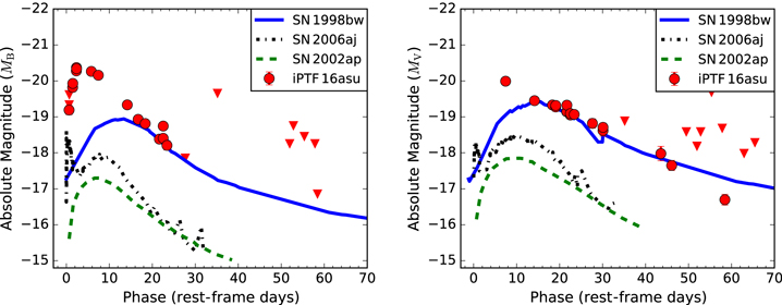
Figure 16. Left: Light curve of iPTF 16asu (red) in the g band, K-corrected to the B band, compared to the light curve of SN 1998bw (blue) in the B band (Galama et al. 1998b; McKenzie & Schaefer 1999), SN 2006aj (black) in the B band (Modjaz et al. 2006; Brown et al. 2014; Bianco et al. 2014), and SN 2002ap (green) in the B band (Foley et al. 2003). Right: Light curve of iPTF 16asu in the r band, K-corrected to the V band, compared to the same SNe, all in the V band.
Download figure:
Standard image High-resolution imageFinally we note that other radioactive species, such as 48Cr and 52Fe, have been proposed to power a class of fast-and-faint thermonuclear transients from He-shell detonations, so-called.Ia SNe (Bildsten et al. 2007; Shen et al. 2010). However, given that iPTF 16asu is 3–5 magnitudes brighter than these models predict, the spectrum at peak is blue and featureless without the expected strong Ti ii features, and the late-time spectrum is an excellent match to SNe Ic-BL, suggesting a core-collapse explosion, we do not consider these models relevant for iPTF 16asu.
6.2. Magnetar
During the core collapse of a massive star, a highly magnetized ( G) rapidly spinning neutron star called a magnetar can be formed. As the newborn magnetar spins down, rotational energy is released and can significantly boost the luminosity of the SN if the spin-down time of the magnetar is comparable to the diffusion time through the ejecta (e.g., Kasen & Bildsten 2010; Woosley 2010; Metzger et al. 2015). Magnetar models have been suggested to explain highly luminous transients, including many SLSNe as well as SN 2011kl (Greiner et al. 2015; Bersten et al. 2016). iPTF 16asu has a luminosity similar to that of to SN 2011kl and some relatively low-luminosity SLSNe (Figures 1 and 5), so we examine whether a magnetar model can explain the peculiar light curve of iPTF 16asu.
As described in Kasen & Bildsten (2010), the hydrodynamic simulations for their magnetar model makes the simplifying assumption that all of the injected energy is thermalized spherically at the base of the ejecta (ignoring the possibility of anisotropic jet-like injection). They further assume homologous expansion, a shallow power-law structure for interior density, and the dominance of radiation pressure. An expanding bubble with a thin shell of swept-up ejecta and a low-density interior are formed due to central overpressure in the SN remnant but rarely affect the outer layers of the SN ejecta. At late times the energy injected by the magnetar continues to heat the ejecta, as in 56Ni decay, but it is no longer dynamically important. This process significantly affects the SN light curve.
The shape of the light curve in magnetar models depends on three parameters: P, the initial spin period; B, the strength of the magnetic field; and  , the diffusion timescale that is proportional to
  . Using the magnetar model fitting code from Kangas et al. (2017) we recover the parameters
  Gauss,
  ms, and
  days. Manually tweaking the parameters slightly to obtain a better visual fit, we show the resulting fit to the bolometric light curve in Figure 17 with the parameters
  ms,
ms,  G, and
  days, and assuming an opacity of
  cm2 g−1. As done in the 56Ni model, the diffusion time and average velocity from the blackbody fits are used to calculate an ejecta mass of
  M⊙. The parameters allow for the energy and the timescale to essentially be tuned separately, making the magnetar model quite flexible and generating a tight fit to both the peak and the decay of the bolometric light curve.
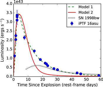
Figure 17. Model 1, the magnetar model best fit to the full light curve, shown in dashed green. Parameters are  ms,
ms,  Gauss, and
  days. Model 2, the magnetar model best fit with constrained
  M⊙, shown as a red line. Parameters are
  ms,
ms,  Gauss, and
  days. The pseudobolometric light curve using
  bands of SN 1998bw (Clocchiatti et al. 2011) is plotted in dotted black to demonstrate how 56Ni decay may power the late-time light curve.
Download figure:
Standard image High-resolution imageAlthough the magnetar model produces a light curve that fits iPTF 16asu, the derived ejecta mass of our best fit is very low. Arcavi et al. (2016) derived similarly small ejecta masses for their rapidly rising SNe events, which caused them to conclude that the magnetar model was unlikely, while Greiner et al. (2015) concluded that a magnetar was a likely explanation for SN 2011kl despite their low derived ejecta mass. For an SN Ic-BL caused by the core collapse of a massive star, a magnetar model with such a low ejecta mass would require an extreme stripping scenario to reduce the core mass. Furthermore, the Kasen & Bildsten (2010) magnetar model was tuned to an ejecta mass of  M⊙ and it is not clear that the assumptions of this model would remain valid in this low-mass regime.
Another way for a magnetar model to produce a fast timescale peak, similar to that of iPTF 16asu, is to use a small period and a high magnetic field, thereby decreasing the spin-down time. When constraining the ejecta mass to be  M⊙, we find the best-fit parameters
  ms,
ms,  Gauss, and
  days. This fit is shown as a red line in Figure 17 and can also reproduce the fast rise and luminous peak of iPTF 16asu. However, this model declines too quickly to explain the entire light curve, so one would need a two-component model (e.g., with the late-time powered by 56Ni, as was considered by Bersten et al. 2016 for SN 2011kl). Thus despite the compelling light curve fit, we conclude that a magnetar model is unlikely to be the sole power source of iPTF 16asu but remains a candidate for powering the peak emission if the late time light curve is powered by 56Ni.
6.3. Off-axis GRB
Long GRBs are often associated with SNe Ic-BL, though not every SN Ic-BL has an accompanying GRB (see, e.g., Woosley & Bloom 2006 for a review of the GRB-SN connection). GRBs are extremely energetic, relativistic, and highly beamed explosions characterized by an initial flash of gamma-rays followed by an "afterglow" of radiation typically seen at wavelengths ranging from the X-ray to the radio. iPTF 16asu's spectra and velocities are similar to those of SNe Ic-BL associated with GRBs (Section 4, Figures 11 and 12), so we examine whether the excess blue emission at peak could be explained as a GRB afterglow.
Nondetections of iPTF 16asu in the X-ray and radio strongly constrain the allowable GRB parameter space. The upper limits from three epochs of Swift data are shown in the left panel of Figure 18. While data at earlier times would have been more constraining, the upper limits rule out the bulk of observed X-ray afterglows with  erg; however, weak or off-axis GRBs are not excluded by the X-ray data alone. Similarly, the right panel shows the upper limits from our two epochs of VLA data. As evident from this figure, we can exclude a radio counterpart to iPTF 16asu as luminous as SN 1998bw or SN 2009bb, but we cannot exclude a lower-luminosity and/or faster-evolving radio counterpart such as SN 2006aj and SN 2010bh. If iPTF 16asu is associated with a GRB, then these limits suggest that it must be a faint (
 erg) event. These constraints are consistent with the analysis from all-sky gamma-ray monitors (Section 2.6), as an on-axis burst at the distance of iPTF 16asu with (
 erg) would have been seen by KW or SPI-ACS.
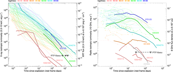
Figure 18. X-ray (left) and radio (right) light curves of long-duration gamma-ray bursts, shifted to the redshift of iPTF 16asu and plotted alongside our measured upper limits for that event from Swift and the VLA. X-ray light curves are from the Swift XRT online database (Evans et al. 2007) plus Tiengo et al. (2004); radio light curves are from the compilation of Chandra & Frail (2012) plus the relativistic SN 2009bb (Soderberg et al. 2010). Light curves are color-coded by the measured isotropic-equivalent gamma-ray luminosity of the prompt emission; see Perley et al. (2014) for additional details. Dashed lines (on the radio plot) indicate upper limits, and some prominent events are highlighted. The upper limits on iPTF 16asu rule out most of the parameter space for previously observed GRB afterglows but permit a faint event similar to GRB 060218.
Download figure:
Standard image High-resolution imageThe most unusual characteristic of iPTF 16asu is its abrupt four-day rise time in the optical. Such a rise time is extremely short in an SN context but would be unprecedentedly long in an SN-GRB context, even though optical afterglow light curves do sometimes show a rise (e.g., GRB 970508; Galama et al. 1998a). To explain the shape of the optical light curve as a GRB afterglow, we therefore consider off-axis GRB models.
From the New York University Afterglow Library data set of off-axis long GRBs at an observed wavelength of 3000 Å (1015 Hz), the models can reproduce a three- to six-day rise for an observer angle of between 23° and 17°, respectively (van Eerten et al. 2010). The data set assumes a jet energy of 2 × 1051 erg, a jet half opening angle of 11 5, and a homogeneous circumburst number density of 1 cm−3. The parameters for an observer angle of 17° produce a light curve with roughly the same peak magnitude as iPTF 16asu; however, in changing to an observed wavelength of 30 mm (10 GHz), these parameters produce a radio light curve that is orders of magnitude brighter than our radio limits. Similarly, considering the low-energy models from van Eerten & MacFadyen (2011), we find that parameters that satisfy the radio limits are inconsistently faint in the optical. The coarse grid of parameters used in van Eerten et al. (2010) does not allow us to make precise comparisons to their model but indicates that while a four-day optical rise could be constructed, our optical light curve and radio upper limits cannot be simultaneously satisfied by current models. A more thorough exploration of energy and density parameter space than is available in these model grids is necessary to determine whether GRB models can account for both the bright optical emission and the lack of X-ray and radio emission.
A similar conclusion can be reached by comparing the observed spectral properties of iPTF 16asu to typical GRB afterglows, which are well described by synchrotron radiation resulting in both a light curve and a spectrum consisting of several power-law segments with associated indices (e.g., Sari et al. 1998). If the featureless blue spectra of iPTF 16asu are due to a GRB afterglow then we expect the spectrum to follow a power law ( ), with typical values of the power-law index β around 0.5–0.6 (e.g., Kann et al. 2010). Fitting our first spectrum (at +3 days after explosion) with a power law, we find a best-fit index of
  , i.e.,
  , which is inconsistent with a GRB-like spectrum. In contrast, the spectrum is well fit by a blackbody (Figure 6). Similarly, if we compare our earliest X-ray upper limit to the corresponding point on the r band light curve, then we derive a limit on the optical- to-X-ray spectral index
  whereas typical GRB afterglows show
  (Gehrels et al. 2008). We also note that the decline of the light curve is better fit by exponential decay than by a power law (Section 3.4, Figure 8 (right)).
While the properties of the luminous blue peak of iPTF 16asu do not seem to resemble a classical GRB afterglow (on- or off-axis), it is worth noting that low-luminosity GRBs like 060218 and 100316D have shown thermal emission in addition to the weak synchrotron component (e.g., Campana et al. 2006; Starling et al. 2011). Thus it is still possible that iPTF 16asu could be a related phenomenon but with a significantly brighter thermal component. The origin of the thermal emission in low-luminosity GRBs is debated, though one possibility is that it is associated with shock breakout. We consider next whether such a model can also explain iPTF 16asu.
6.4. Shock Cooling
The short timescales and blue colors of iPTF 16asu are reminiscent of shock cooling transients, where the early light curve of an SN is powered by the cooling of the envelope following the breakout of the SN shock, usually followed by a second peak from the SN itself (e.g., SN 1993J; Wheeler et al. 1993). Such a shock cooling phase should be present in all SNe (Nakar & Sari 2010), but both the duration and the luminosity will depend on the structure of the progenitor star. A peak in both the red and blue bands, as we see in iPTF 16asu, is generally associated with shock breakout from extended material (Nakar & Piro 2014). Shock cooling models have been considered for other rapidly evolving transients (e.g., Ofek et al. 2010; Drout et al. 2014) as well as low-luminosity GRBs (e.g., Nakar 2015), so we consider here whether iPTF 16asu could be explained by a shock cooling scenario.
Since the peak is seen in all bands, we consider the extended envelope model of Nakar & Piro (2014). Here the mass in the extended envelope scales as  and the effective radius of the material scales as
  . For the rise time and peak luminosity measured for iPTF 16asu, this suggests an envelope mass of around ∼0.5 M⊙ and a lower limit on the effective radius of the material of
  cm, still assuming
  cm2 g−1.
Piro (2015) developed this extended envelope further, and Figure 19 shows a fit of the model with the parameters  M⊙,
M⊙,  cm, and
  erg. In general there is a degeneracy between the initial radius of the material and the energy deposited by the shock, but our high observed velocities suggest that we are in the regime of a smaller radius and higher energy (Piro 2015). Since the energy deposited into the extended material is just a fraction of the total SN energy, if this model is correct then it would imply a very high explosion energy, likely requiring a central engine.
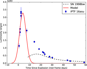
Figure 19. Fit of shock-breakout model (red) from Piro (2015) using the parameters  cm2 g−1,
  M⊙
M⊙  cm (
cm ( ), and
  erg. The pseudobolometric light curve using
  bands of SN 1998bw (Clocchiatti et al. 2011) is plotted in black to illustrate how 56Ni decay could power the late-time light curve.
Download figure:
Standard image High-resolution imageUnlike many shock-breakout SNe, iPTF 16asu exhibits only a single peak, so if the main light curve peak is powered by shock cooling then it must completely dominate the contribution from the underlying normal SN light curve. The model shown in Figure 19 approximates the shock cooling light curve with a Gaussian and is not expected to capture the decline of the light curve, which would depend on the density structure of the material. It does, however, demonstrate that an extended envelope model can produce a peak with a rise time and luminosity compatible with iPTF 16asu. As seen in Figure 16, an SN Ic-BL slightly less luminous than SN 1998bw could be hidden underneath a luminous shock-breakout peak forming one continuous peak by the merging of the second SN peak with the decay of the first peak.
In Nakar (2015), SN 2006aj/GRB 060218 was modeled by a shock breakout from energy deposited into an extended ( ) low-mass (
 M⊙) envelope by a low-luminosity GRB. Thus iPTF 16asu could have a similar explosion mechanism but with a significantly higher-mass envelope, producing a longer-duration and luminous peak. The presence of circumstellar material would also be consistent with the constraints on high-energy emission; indeed, it has been suggested that low-energy soft GRBs like 060218 and 100316D have extended circumstellar material (Margutti et al. 2015).
7. Summary
We present photometric and spectroscopic observations of the unique transient iPTF 16asu. The key observed properties can be summarized as follows:
- 1.A rapidly evolving and luminous light curve, with a rise of 4.0 days to a high peak luminosity of
 erg s−1. The decline is similarly fast and is well fit by exponential decay with a characteristic timescale of 14 days.
 - 2.A blue and featureless spectrum near peak that is well fit by a blackbody, using UV and optical data, with a temperature of and a radius of cm.
- 3.Broad spectroscopic features emerging on the decline that are well matched to SNe Ic-BL. The velocities, as measured from the Fe ii Å line, are comparable to SNe Ic-BL with accompanying GRBs.
- 4.Nondetections in the X-ray (Swift/XRT) corresponding to limits of erg s−1 and in the radio (VLA) corresponding to limits of erg s−1. Nondetections by all-sky gamma-ray monitors similarly constrain any associated on-axis GRB to be low-energy ().
- 5.A dwarf host galaxy, with a stellar mass of, a metallicity of , and a star formation rate of .


We discuss various energy sources to explain the above observed properties. We find that 56Ni decay, as in an ordinary SN Ic-BL, is adequate to explain the late-time photometry. It is also consistent with the observed spectra and nondetections in the X-ray and radio bands. However, attempting to fit the rapid rise and luminous peak solely with 56Ni decay gives the unphysical result that  . Hence we consider two different hypotheses to explain the early data.
First we consider a magnetar model. The magnetar model either requires a very small ejecta mass ( ) in order to fit the sharp rise or a high magnetic field (
 G) that decreases the spin-down time. The latter would require that the late-time data are explained by the radioactive decay of 56Ni.
Next we find that shock cooling can also explain the fast rise and high luminosity with a dense envelope ( M⊙,
M⊙,  cm) and high injected energy (
 erg). The required energetics in this model also implies an underlying central engine. Shock cooling through the envelope has been seen in the low-luminosity SN 2006aj/GRB 060218. Our spectra and kinematics are also more similar to SNe Ic-BL associated with GRBs. Our radio and X-ray limits constrain the energy (
 ) of any associated GRB to be
  . Regardless of whether or not there was a GRB, the late-time light curve is reasonably fit by 56Ni decay.
Both of the above scenarios suggest that iPTF 16asu was an engine-driven SN, making it an intriguing transition object between SLSNe, low-luminosity GRBs, SNe Ic-BL, and objects like SN 2011kl. We hope that new discoveries from the next generation of wide-field surveys (e.g., Zwicky Transient Facility; Bellm & Kulkarni 2017) will enable us to find more objects like iPTF 16asu and more conclusively determine the origins of such fast and luminous transients.
We thank the anonymous referee for constructive comments that improved the manuscript. We thank Iair Arcavi, Maria Drout, Avishay Gal-Yam, Raffaella Margutti, and Maryam Modjaz for helpful discussions and comments. R. L. acknowledges helpful discussions at the Munich Institute for Astro- and Particle Physics (MIAPP) workshop "Superluminous Supernovae in the Next Decade," supported by the MIAPP, of the DFG cluster of excellence "Origin and Structure of the Universe." We thank Harish Vedantham, Vikram Ravi, and Anna Ho for assisting with the observations presented in this paper. The Intermediate Palomar Transient Factory project is a scientific collaboration among the California Institute of Technology; Los Alamos National Laboratory; the University of Wisconsin, Milwaukee; the Oskar Klein Center; the Weizmann Institute of Science; the TANGO Program of the University System of Taiwan; and the Kavli Institute for the Physics and Mathematics of the Universe. This work was supported by the GROWTH project, funded by the National Science Foundation under Grant No. 1545949. This work is partially based on data acquired with the Swift GO program 1215281 (Grant No. NNX16AN84G, PI: R. Lunnan). Part of this research was carried out at the Jet Propulsion Laboratory, California Institute of Technology, under a contract with NASA. The National Radio Astronomy Observatory is a facility of the National Science Foundation operated under cooperative agreement by Associated Universities, Inc. A. C. acknowledges support from the National Science Foundation CAREER Award No. 1455090. D. S. and D. F. gratefully acknowledge support from RSF Grant No. 17-12-01378. This work made use of the data products generated by the New York University SN group and released under doi: 10.5281/zenodo.58767, available at https://github.com/nyusngroup/SESNspectraLib based on observations made with the Nordic Optical Telescope, operated by the Nordic Optical Telescope Scientific Association at the Observatorio del Roque de los Muchachos, La Palma, Spain, of the Instituto de Astrofisica de Canarias. Some of the data presented herein were obtained at the W. M. Keck Observatory, which is operated as a scientific partnership among the California Institute of Technology, the University of California, and NASA. The Observatory was made possible by the generous financial support of the W. M. Keck Foundation. The authors wish to recognize and acknowledge the very significant cultural role and reverence that the summit of Mauna Kea has always had within the indigenous Hawaiian community. We are most fortunate to have the opportunity to conduct observations from this mountain.
Facilities: PO: 1.2 m - , PO: 1.5 m - , PO: Hale - , Keck: I - , Keck: II - , NOT - , TNG - , Swift - , VLA - .
Footnotes
- 18
IRAF is distributed by the National Optical Astronomy Observatory, which is operated by the Association of Universities for Research in Astronomy under a cooperative agreement with the National Science Foundation.
- 19
- 20