


Abstract
We use data on gas temperature and velocity dispersion from the Green Bank Ammonia Survey and core masses and sizes from the James Clerk Maxwell Telescope Gould Belt Survey to estimate the virial states of dense cores within the Orion A molecular cloud. Surprisingly, we find that almost none of the dense cores are sufficiently massive to be bound when considering only the balance between self-gravity and the thermal and non-thermal motions present in the dense gas. Including the additional pressure binding imposed by the weight of the ambient molecular cloud material and additional smaller pressure terms, however, suggests that most of the dense cores are pressure-confined.
Export citation and abstract BibTeX RIS
1. Introduction
Dense cores, condensations of gas and dust ∼0.1 pc in size, are the birthplaces of stars (e.g., Bergin & Tafalla 2007; Di Francesco et al. 2007; Ward-Thompson et al. 2007a). One of the most important properties of a dense core is its degree of stability against gravitational collapse. Understanding which subset of cores in a molecular cloud population is likely to form protostars in the near future, versus which subset of cores is likely to not form protostars soon (or ever, unless local conditions change) has profound implications for star formation efficiency and the interpretation of the core mass function. Detailed studies of individual cores (including full 3D modeling, e.g., Steinacker et al. 2013) are essential for accurately determining all properties of an individual system. This approach, however, requires a prohibitive amount of data and modeling time for cloud-wide studies of core populations. Instead, by adopting simple stability proxies, insight can be gained into the global properties and variations of cores within a molecular cloud. Even this approach requires a non-negligible amount of information, including mass, temperature, non-thermal motions, and other properties that are typically estimated from different types of observations. The Green Bank Ammonia Survey (GAS; Friesen et al. 2017) provides an important contribution to these studies. Using the Herschel (André et al. 2010) and James Clerk Maxwell Telescope (JCMT) (Ward-Thompson et al. 2007b) Gould Belt Surveys to identify areas of high extinction within nearby molecular clouds (<500 pc) that likely have dense gas, GAS data provide information on gas temperature and velocity to complement that on (dust) column density collected by the Gould Belt Surveys. The large and uniform areal coverage of these three surveys provides an unprecedented opportunity to understand the broad stability properties of dense structures formed within nearby molecular clouds.
The Orion A molecular cloud is one of the most distant clouds covered by GAS and is located at a distance of ∼415 pc from the Sun (Menten et al. 2007; Kim et al. 2008). Orion A is also the closest example of a molecular cloud forming high-mass stars. For example, there are several O stars forming within the Orion Nebula Cluster (e.g., Hillenbrand 1997; Bally 2008). The Orion A complex also hosts hundreds of mostly lower mass protostars (e.g., Megeath et al. 2012; Stutz et al. 2013) and many dense cores forming, or with the potential to form, additional protostars (e.g., Mezger et al. 1990; Johnstone & Bally 1999; Ikeda et al. 2007; Li et al. 2007; Sadavoy et al. 2010; Shimajiri et al. 2011; Polychroni et al. 2013; Salji et al. 2015; Lane et al. 2016; Mairs et al. 2016). The large census of dense cores, and extensive observations available for the region, in combination with its status as the nearest higher-mass star-forming region, make Orion A an ideal cloud in which to investigate core properties and boundedness.
The dense cores within the OMC2 and OMC3 regions of Orion A (i.e., the top portion of the integral shaped filament (ISF)) have previously been analyzed from a virial perspective by Li et al. (2013), using a combination of SCUBA data from Nutter & Ward-Thompson (2007) to identify the dense cores and NH3 data from the Very Large Array (VLA) and Green Bank Telescope (GBT) to estimate the velocity dispersion and kinetic temperature. While the spatial resolution of the NH3 data is quite good, 5'', the spectral resolution is poor, with an FWHM of 0.6 km s−1, and Li et al. (2013) find that many of the dense cores have intrinsic line widths below their resolution.
Given the better velocity resolution and larger spatial coverage of our GAS observations, it is worth revisiting a virial analysis of Orion A. Here, we combine data from the JCMT Gould Belt Survey (GBS), which identified dense cores and characterized their basic properties (size and mass), with new dynamical data from GAS, which trace the motions of the dense gas (NH3) associated with these dense cores.
In Section 2, we present the GAS and JCMT GBS observations used in our analysis, along with supplementary publicly available data (e.g., protostellar catalogs and maps of total cloud column density). In Section 3, we first perform a simple virial analysis comparing only self-gravity with thermal and non-thermal support, and find that most of the dense cores appear unbound under these assumptions. We then include confining pressure terms in our analysis and show that most of the cores are actually bound. In Section 4, we discuss our results in the context of external pressure binding being an important ingredient in all nearby star-forming regions, before concluding in Section 5.
2. Observations
2.1. GBT NH3 Observations
NH3 observations were obtained through the GAS, a large project to map the ammonia (1, 1), (2, 2), and (3, 3) rotation-inversion transitions across the high-extinction regions of nearby Gould Belt molecular clouds using the Green Bank Telescope's K-band Focal Plane Array. The survey strategy, data reduction procedure, and basic data properties are described in detail in Friesen et al. (2017). The spatial resolution is 32'' (0.064 pc), while the spectral resolution is 0.07 km s−1. The northern portion of the Orion A cloud is one of the first four areas mapped, and observations of it are presented in Friesen et al. (2017) as "Data Release 1" (DR1).15 The DR1 observations of Orion A cover the ISF and areas slightly southward of it. Additional data further south were obtained at a later date and will be included in a second data release. Figure 1 shows an overview of the area mapped overlaid on the JCMT SCUBA-2 850 μm image of the region, with the dense cores (see Section 2.2) and protostars (see Section 2.3) overlaid in each panel.

Figure 1. Overview of the JCMT GBS 850 μm data over the portion of Orion A observed by GAS. The blue contour shows the areal coverage of GAS for the present DR1 analysis. In the left panel, the dark orange circles show young stellar objects (YSOs) identified using Spitzer data (Megeath et al. 2012), while the filled yellow triangles show additional YSOs identified using Herschel data (Stutz et al. 2013). In the right panel, the ellipses show the Gaussian 1σ contours fit to the culled getsources core catalog of Lane et al. (2016). Here, protostellar cores are shown in red while starless cores are shown in green.
Download figure:
Standard image High-resolution image2.2. JCMT SCUBA-2 Data
Although NH3 is an excellent tracer of dense gas, defining dense cores from its emission alone can be complicated by varying abundance levels. At the distance of Orion (∼415 pc; Menten et al. 2007; Kim et al. 2008), the ∼32'' resolution of our GAS data also presents a challenge in identifying individual dense cores in such a complex and clustered environment. Submillimeter continuum emission offers an alternative method for identifying dense cores and estimating their sizes and masses. There are, however, several separate significant sources of uncertainty in the conversion between flux density and mass, as well as the potential for chance alignments of lower-density structures giving rise to apparent cores. The JCMT GBS (Ward-Thompson et al. 2007b) observed 6.2 square degrees around the Orion A molecular cloud at 850 μm and 450 μm with SCUBA-2, with resolutions of 14 6 and 98 (Dempsey et al. 2013), respectively. Observations of the northern and southern portions of Orion A were first published in Salji et al. (2015) and Mairs et al. (2016), respectively. For our analysis, we use the dense core catalog presented in Lane et al. (2016), which covers the entire Orion A complex.
Lane et al. (2016) analyzed the JCMT GBS 850 μm data for the entire Orion A molecular cloud, using a map that reaches the full survey depth but is slightly poorer at recovering the largest-scale structures than the current best reduction method. Lane et al. (2016) identified dense cores using two independent methods, getsources (Men'shchikov et al. 2012) and FellWalker (Berry 2015), and analyzed their clustering properties. The getsources algorithm is a multi-scale, multi-wavelength source extraction algorithm. It first decomposes emission from each wavelength into a variety of scales, and then uses the combined information across wavelengths to create a Gaussian-based model that characterizes the small-scale sources and separates them from larger-scale emission features. In contrast, the FellWalker algorithm separates peaks based on local gradients, assigning each pixel to the peak that the local gradient points toward. FellWalker therefore does not assume any particular source geometry, and in the Lane et al. (2016) catalog, no background subtraction was performed to remove large-scale structures. Since Orion A is home to quite complex emission structures, Lane et al. (2016) found that in general getsources performed better in isolating dense and compact structures. For our main analysis, we therefore adopt the getsources-based catalog of Lane et al. (2016), although in Appendix A, we present an analysis using instead the FellWalker-based catalog. In Appendix A, we demonstrate that our results are robust against changes in the core catalog used.
The Orion A catalog of Lane et al. (2016) provides the sizes, total fluxes, and peak positions of the dense cores. We approximate the dense core radius as the geometric mean of the major and minor axis FWHMs fit by getsources, noting that at a radius equal to the FWHM, a Gaussian profile is at one eighth of its full height, and is therefore a reasonable estimate of the full core extent. We assume a distance of 415 pc to Orion A, and correct the catalog values of Lane et al. (2016) from their assumed distance of 450 pc. We also correct the core sizes for the telescope beam; for cores with sizes less than half of the 146 FWHM of the SCUBA-2 850 μm beam, deconvolution is likely to be unreliable, and so we report this value as the upper limit to their true size. We convert the total flux of each core measured by getsources to a mass using
where S850 is the total flux density at 850 μm,  is the dust opacity at 850 μm, Td is the dust temperature, and D is the distance. We assume a constant dust grain opacity at 850 μm of 0.012 cm2 g−1, consistent with previous JCMT and Herschel Gould Belt analyses, and which includes the standard dust-to-gas ratio of 0.01 (e.g., Kirk et al. 2013; Pattle et al. 2015). (Note that the popular model 5 of Ossenkopf & Henning (1994) for icy grains would give a larger opacity of 0.018 cm2 g−1 at 850 μm.) For each core, we adopt a dust temperature equal to the kinetic temperature derived from our GAS NH3 observations (see Section 2.4). For cores where a kinetic temperature could not be measured, we assume a value of 18 K, which is the mean temperature measured for the cores in NH3. Previous works, including Lane et al. (2016), assumed a constant dust temperature of 15 K, which would give masses roughly 30% larger than those quoted here for a mean dust temperature of 18 K. Similarly, assuming instead a higher temperature of 21 K would give masses that were 20% smaller. We note that while a 20%–30% change in estimated mass can be significant for a detailed study of a single object, this level of difference has relatively little impact on our population study because of the broad range in properties measured. For example, most of the cores would not change their status of being gravitationally bound or unbound in Section 3.2 with only a 20%–30% change in their mass. Much larger variations in the mass estimated for cores arise in regions of complex emission structure such as Orion A through the choice in algorithm used to identify cores. In Appendix A, the cores identified using FellWalker tend to be more massive and larger than the getsources cores. Highlighting the challenges of core identification, there is not always a one-to-one correspondence between objects in the two catalogs, because getsources tends to split emission structures more finely than FellWalker does. Despite these large uncertainties in defining individual cores and accurately measuring their properties, our overall conclusions about the typical virial state of cores are similar using either algorithm, suggesting that our overall conclusions about bulk virial properties are robust.
Finally, we note that some of the dense cores in Lane et al. (2016), although they are clearly detected, have poor Gaussian fits. While this was not important for the original clustering analysis of Lane et al. (2016), poor estimates of the core radius could significantly impact our virial analysis. We therefore apply several cuts to the getsources catalog of Lane et al. (2016), requiring dense cores in our present analysis to have parameters:
- gs_sig_glob ≥ 1
- gs_sig_mono8 ≥ 7
- gs_good > 0
- gs_relp850 > 3
- gs_relt850 > 3.
In short, these criteria imply "significant" fits (gs_sig_glob, gs_sig_mono8) with fitted peak fluxes of signal-to-noise ratio (S/N) ≥ 3 (gs_relp850) and fitted total fluxes of S/N ≥ 3 (gs_relt850), and no getsources flags (gs_good) associated with the fits. These fitting criteria reduce the original 919 dense cores in Lane et al. (2016) to 610, primarily excluding the faintest cores with the poorest fits. In the culled catalog, the lowest mass core identified is 0.09  . Of the 610 reliably fit dense cores, roughly half (311) lie within the area mapped by GAS. The median mass of the cores is 0.7
  for those with reliable getsources sizes and reliable temperature and kinematic measures (see Section 2.4).
Figure 1 shows the GBS 850 μm emission over the area observed with GAS, with the culled getsources catalog overlaid. The dearth of getsources cores in the center of the ISF visible in Figure 1 is caused by two effects. First, getsources excludes large-scale emission modes from its core-fitting routine, and hence a significant amount of flux within the center of the ISF is not attributed to any getsources core. Second, the larger-scale emission within the center of the ISF increases the difficulty of fitting Gaussian models to the compact emission features present, leading to a greater fraction of cores being culled in this particular area. We note, however, that our overall results are similar even when the full getsources catalog from Lane et al. (2016) is used.
In Table 1, we summarize the properties of the cores identified by getsources for which there are measurements of their GAS-derived properties (see following sections).
Table 1. Properties of the Dense Cores
| IDa | R.A.a | Decl.a | Ma | Reffa | Ca | Pr?a |
 (km s−1)b (km s−1)b
|
Tkin(K)b |
 c
c
|
Virial |
 d
d
|
 d
d
|
||||
|---|---|---|---|---|---|---|---|---|---|---|---|---|---|---|---|---|
| (J2000) | (J2000) | ( ) ) |
(pc) | mean | err | std | mean | err | std | log(K cm−3) | Ratiod | |||||
| 5 | 83.84726 | −5.02459 | 8.28 | 0.017 | 0.64 | Y | 0.311 | 0.002 | 0.041 | 17.5 | 0.1 | 0.8 | 7.3 | 1.4E+00 | 2.6E+00 | 2.0E+01 |
| 9 | 83.86135 | −5.16620 | 11.10 | 0.023 | 0.48 | Y | 0.435 | 0.001 | 0.067 | 23.3 | 0.1 | 1.5 | 7.3 | 8.2E-01 | 1.5E+00 | 1.1E+01 |
| 10 | 83.82113 | −5.32181 | 4.92 | 0.017 | 0.51 | N | 0.542 | 0.001 | 0.075 | 25.2 | 0.0 | 0.8 | 7.5 | 3.9E-01 | 6.2E-01 | 4.2E+00 |
| 12 | 83.81898 | −5.32483 | 3.84 | 0.017 | 0.58 | N | 0.517 | 0.001 | 0.084 | 25.5 | 0.0 | 1.0 | 7.5 | 3.7E-01 | 5.2E-01 | 2.5E+00 |
| 16 | 83.81604 | −5.33532 | 2.06 | 0.025 | 0.69 | N | 0.477 | 0.001 | 0.084 | 28.1 | 0.0 | 1.5 | 7.5 | 8.5E-01 | 2.1E-01 | 1.4E-01 |
| 17 | 83.82469 | −5.31807 | 2.93 | 0.017 | 0.54 | N | 0.563 | 0.001 | 0.064 | 25.2 | 0.0 | 0.9 | 7.5 | 2.9E-01 | 3.5E-01 | 1.6E+00 |
| 18 | 83.81026 | −5.31189 | 3.64 | 0.026 | 0.62 | N | 0.450 | 0.001 | 0.109 | 23.7 | 0.0 | 0.8 | 7.4 | 6.1E-01 | 4.1E-01 | 5.0E-01 |
| 19 | 83.86445 | −5.15861 | 3.11 | 0.027 | 0.63 | Y | 0.423 | 0.001 | 0.074 | 23.7 | 0.1 | 1.7 | 7.3 | 5.8E-01 | 3.8E-01 | 4.8E-01 |
| 21 | 83.84284 | −5.01978 | 3.61 | 0.017 | 0.56 | Y | 0.272 | 0.001 | 0.052 | 17.0 | 0.1 | 0.7 | 7.3 | 8.5E-01 | 1.3E+00 | 3.7E+00 |
| 23 | 83.82478 | −5.00483 | 2.49 | 0.017 | 0.62 | N | 0.341 | 0.001 | 0.033 | 17.8 | 0.0 | 0.4 | 7.2 | 5.2E-01 | 6.9E-01 | 1.9E+00 |
Notes.
aCore properties based on the getsources catalog of Lane et al. (2016). Only cores that have kinematic properties measured by GAS are listed. Columns are the core ID in Lane et al. (2016), central position, mass (estimated using Equation (1) from the total flux), effective radius (geometric mean of the major and minor axis lengths), concentration as derived using Equation (11) and whether the core has an associated protostar. bVelocity dispersion ( ) and kinetic temperature (Tkin) measured for the cores, averaging over all core pixels where sufficient signal was present. The value reported for each quantity is the mean weighted by the inverse square of the uncertainty. The formal error in the weighted mean value is also reported (second column), as is the weighted standard deviation (third column). This latter quantity is more reflective of the variation between fitted values across the core.
cEstimated pressure on the core boundary due to the weight of the overlying cloud material. See Section 3.2 for more information.
dVirial parameters estimated according to Section 3.2. The virial ratio is given by
) and kinetic temperature (Tkin) measured for the cores, averaging over all core pixels where sufficient signal was present. The value reported for each quantity is the mean weighted by the inverse square of the uncertainty. The formal error in the weighted mean value is also reported (second column), as is the weighted standard deviation (third column). This latter quantity is more reflective of the variation between fitted values across the core.
cEstimated pressure on the core boundary due to the weight of the overlying cloud material. See Section 3.2 for more information.
dVirial parameters estimated according to Section 3.2. The virial ratio is given by  .
.  reflects the balance of gravitational binding versus thermal pressure, while
  reflects whether gravity or external cloud pressure dominates the confinement of the cores.
Only a portion of this table is shown here to demonstrate its form and content. A machine-readable version of the full table is available.
Download table as: DataTypeset image
2.3. Protostars
Lane et al. (2016) further classify their dense cores as being protostellar or starless based on whether or not they are spatially coincident with a protostar identified by Megeath et al. (2012) using Spitzer observations or by Stutz et al. (2013) using Herschel data. Due to the highly clustered nature of Orion A, Lane et al. (2016) required a separation of less than one beam radius (725) from the location of the dense core's peak for a core to be classified as protostellar. Note that this requirement of a small separation ensures that any given protostar can be associated with a maximum of one dense core. Meingast et al. (2016) recently identified YSOs in Orion based on near-infrared observations using VISTA. We searched their catalog for evidence of additional protostellar cores, but found only three possible new associations with our core catalog, all of which were listed in Meingast et al. (2016) as previously known class II sources. For simplicity, we did not reclassify these three cores. Protostellar and starless dense cores are shown in Figure 1 in the right panel, while the protostars themselves are shown in the left panel.
2.4. Deriving Dynamical Core Properties
The GAS NH3 (1, 1) and (2, 2) observations were used to estimate the properties of the dense gas, as described in more detail in Friesen et al. (2017). Our interest here is in the velocity dispersion, σ, and the kinetic temperature, Tkin. Figure 2 shows a comparison of Tkin overlaid with the SCUBA-2 850 μm emission of Orion A, highlighting the well-known fact that the most active part of the ISF tends to be noticeably warmer than its surroundings. We note that for the GAS DR1, all spectra are fit with a single velocity component. A visual inspection of the spectra suggests that a single velocity component is sufficient to describe the majority of NH3 spectra, even in Orion A; however, several per cent of the spectra require a second velocity component to be well described (Friesen et al. 2017). Fits with multiple velocity components are planned for a future GAS data release.

Figure 2. Comparison of the GBS 850 μm data in Orion A (grayscale) with the kinetic temperature of NH3 fitted to the GAS data (colorscale). The SCUBA-2 flux scale is the same as in Figure 1, while Tkin varies from 5 K (blue) to 30 K (red) in the color scaling (see color bar).
Download figure:
Standard image High-resolution imageUsing the GAS NH3-based property maps, we calculate the weighted mean kinetic temperature and velocity dispersion of each dense core. For the getsources-based dense core catalog used for the bulk of our analysis, we consider all GAS pixels that lie within a radius of one core FWHM from each core's peak (i.e., the same area as the core's full extent, as discussed in Section 2.2), and calculate the weighted mean of each property (weighting by the inverse square of the uncertainty in the fitted parameter). We calculate both the error in the weighted mean as well as the weighted standard deviation, to measure the variation in property values across each core. These values are all listed in Table 1. We also measured the kinetic temperature and line width at the peak position for all of the cores, and found largely similar results to those presented here. A total of 29 protostars and 282 starless cores lie within the GAS observing footprint. Of these, 26 protostars and 211 starless cores have kinematic properties measured, i.e., there was sufficient sensitivity in the ammonia data to estimate line widths and kinetic temperatures. The velocity dispersions are similar for the starless and protostellar cores, with a mean and standard deviation of 0.38 km s−1 ± 0.20 km s−1 and 0.37 km s−1 ± 0.17 km s−1, respectively. The kinetic temperatures are also similar. After removing less reliable measures where  K, we find typical kinetic temperatures of 18 K ± 4 K for the starless cores, and 17 K ± 3 K for the protostellar cores. Previous observations have tended to find smaller kinetic temperatures for starless cores than for protostellar cores—for example, Jijina et al. (1999) compiled all available NH3 observations in the literature and found median values of the kinetic temperature of 12.4 K and 15 K for apparently starless and protostellar cores respectively, while more recent work in the Perseus molecular cloud reveals typical kinetic temperatures of 10.6 K and 11.9 K for starless and protostellar cores respectively (Foster et al. 2009). Both Jijina et al. (1999) and Foster et al. (2009) also note that environment appears to play a stronger role than protostellar content in determining the kinetic temperature. Jijina et al. (1999) found median kinetic temperatures of 20.5 K and 12.0 K for cores within and outside clusters, while Foster et al. (2009) measured typical kinetic temperatures of 12.9 K and 10.8 K, for clustered and unclustered cores respectively, in Perseus. Since all of the dense cores we analyze in Orion A lie within a highly clustered environment, we might not expect to see cores with lower kinetic temperatures. This general trend of higher kinetic temperatures being present in more clustered environments is also obvious across the four GAS DR1 regions (Friesen et al. 2017), where the isolated B18 (Taurus) has the lowest kinetic temperatures, and the moderately clustered NGC 1333 (Perseus) and L1688 (Ophiuchus) have intermediate kinetic temperatures. It is possible that our estimated Tkin values in Orion A are also are slightly elevated due to contamination from the warmer envelope material surrounding the dense cores.
2.5. Total Column Density
To estimate the ambient pressure due to the weight of surrounding molecular cloud material on the dense cores, we require a map of the total column density in Orion A. Lombardi et al. (2014) derived such a map by performing point-by-point modeling of the spectral energy distribution of flux measured by both the Planck and Herschel Space Telescopes. We use the 850 μm map of optical depth derived in Lombardi et al. (2014), and convert into column density using the equations and constants given in their Equations (12) and (16):

and

where AK is the extinction in the K-band,  mag,
mag,  mag, Σ is the column density (in mass units),
  ,
,  cm−2 mag−1, and
  g.16
Note that the factors γ and δ are fitted by Lombardi et al. (2014), and they obtain slightly different values in Orion B than in Orion A. We adopt the Orion A values here. The left panel of Figure 3 shows the map of column density from Lombardi et al. (2014) with the scalings above adopted.
g.16
Note that the factors γ and δ are fitted by Lombardi et al. (2014), and they obtain slightly different values in Orion B than in Orion A. We adopt the Orion A values here. The left panel of Figure 3 shows the map of column density from Lombardi et al. (2014) with the scalings above adopted.

Figure 3. Left: original map of column density from Lombardi et al. (2014) shown over the same area as in the previous figures. Contours are shown for  cm−2 and
  cm−2. Right: map of column density containing only structures larger than 0.5 pc. Contours are shown for
  cm−2 and
  cm−2.
cm−2.
Download figure:
Standard image High-resolution imageEvery position in the map of column density may have contributions from structures on a variety of size scales. To estimate the pressure on the cores from the weight of the overlying molecular cloud, we need to consider only the portion of the column density that is attributable to larger-scale structure. In particular, the 36'' angular resolution of the map of column density (matching the Herschel resolution at 500 μm) is comparable to the size of the dense cores, suggesting that in the vicinity of the dense cores, a non-negligible portion of the column density measured could arise from the cores themselves and not from larger-scale structures. We therefore filter out the smallest scale structures from the map of column density when estimating the pressure of the cloud weight. To perform this filtering, we use a similar method to that in Kainulainen et al. (2014). Namely, we use the à Trous wavelet transform to measure the amount of structure on various scales.17
Structures are measured on scales of  pixels, by smoothing and subtracting the smoothed image from the remainder, going from the largest to the smallest scale. The large-scale structure can then be represented as the sum of all single-scale structure maps at sizes above the desired smoothing scale.
In the maps of Lombardi et al. (2014), each pixel is 15'', corresponding to 0.03 pc at a distance of 415 pc. Dense cores tend to have sizes between 0.03 pc and 0.2 pc (Bergin & Tafalla 2007), while larger-scale clumps and clouds span sizes from several tenths of a parsec to more than 10 pc. For a conservative estimate, we assume that the structures of order 0.5 pc and larger belong to the cloud rather than the dense core. The closest smoothing scale to 0.5 pc is 16 pixels, which corresponds to 0.48 pc. For our nominal best estimate of the column density attributable to the cloud, we sum all structures of sizes ∼0.5 pc and larger generated by the à Trous algorithm. In Appendix B, we show that our qualitative conclusions remain similar even when we change the limiting size scale for the features of the cloud column density. Figure 3 shows the original map of column density of Lombardi et al. (2014), as well as the 0.5 pc filtered version of the map, which we use for the majority of our analysis.
Within the large-scale cloud structure, dense cores are also usually found to reside within filaments. Observations from Herschel suggest that filaments have widths of order 0.1 pc (Arzoumanian et al. 2011; André et al. 2014), similar to the size of the dense cores, which makes separating cores and filaments unfeasible using the simple filtering method described above. In our analysis in Section 3.3, we approximate the bounding pressure of filaments using a different method than that discussed here. Finally, we note that not all of the column density may belong to structures that the core is associated with, i.e., some of the column density may belong to additional structures along the line of sight. This is especially important to acknowledge in a region as complex as Orion A. While multiple structures along the line of sight are likely more common at intermediate size scales than at the largest cloud scale, we note that our estimate of the cloud column density may be slightly too high.
3. Analysis
3.1. Line Width–Size Relationship
We first examine the relationship between the line widths and sizes of the dense cores. The observed line width,  , has contributions from both turbulent and thermal energy, i.e.,

We assume that the kinetic temperature for the mean gas is the same as we measure for NH3, and calculate the total line width by subtracting the thermal contribution from NH3 and adding in the assumed total gas thermal contribution, i.e.,
where kB is the Boltzmann constant,  is the molecular weight of NH3 (17),
  the mean molecular weight, and mH the mass of a hydrogen atom. Following Kauffmann et al. (2008), we take
  .
.
Bulk motions within a core can also contribute to the total velocity dispersion, and are usually quantified through measurement of the standard deviation in the centroid velocity of the gas measured across the core. This contribution would then be added to the total velocity dispersion in quadrature. We find that including this term typically has a small effect on the resulting total velocity dispersions, adding less than 0.1 km s−1 to the total velocity dispersion calculated without its inclusion for more than 90% of the cores. The mean difference in the total velocity dispersion between including and excluding the standard deviation in centroid velocity is 0.04 km s−1, while the median difference is 0.02 km s−1. We therefore exclude the contribution from the change in line centroid to the total velocity dispersion that we use for our analysis.
Figure 4 shows the total line width and size measured for each core, using Equation (5). All of the cores have significantly supersonic velocity dispersions—the velocity dispersion expected for a purely thermal gas at the mean Tkin value observed is shown by the horizontal dashed line, and it lies about a factor of two lower than the smallest total velocity dispersions measured. These line widths are larger than is typical for the nearest molecular clouds, such as those in Perseus, where cores tend to have roughly transsonic total line widths (e.g., Foster et al. 2009). Orion, however, has long been recognized as an environment where cores have larger non-thermal motions present in dense gas tracers such as NH3 (e.g., Caselli & Myers 1995; Jijina et al. 1999). These larger line widths do not appear to be an artefact of the larger distance to Orion as compared to nearby clouds such as Perseus. We compared the NH3 line widths reported by Li et al. (2013) using VLA observations of higher angular resolution (∼5'' versus our 32'') and see no evidence that our measured line widths are systematically larger. On the contrary, our measurements tend to be slightly smaller, likely due to the poorer velocity resolution of the observations of Li et al. (2013).
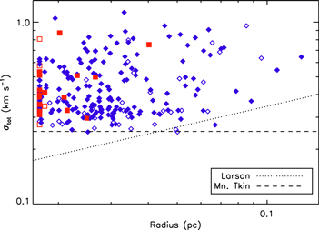
Figure 4. Total 1D velocity dispersion of the dense cores compared with their effective radii. The dashed horizontal line shows the velocity dispersion of purely thermal gas at a temperature equal to the mean kinetic temperature of the cores, i.e., 18 K. The dotted diagonal line shows the line width–size relationship reported by Larson (1981), after scaling for the appropriate observed quantities, i.e., radius vs. diameter and 1D vs. 3D velocity dispersion. Red squares indicate protostellar cores while blue diamonds indicate starless cores. Filled symbols indicate cores lying near the ISF, and open symbols show cores that lie further south.
Download figure:
Standard image High-resolution imageThe dotted diagonal line in Figure 4 shows the standard line width–size relationship of Larson (1981) measured for larger-scale structures using CO observations. Clearly our population of cores does not follow Larson's scaling law, but instead it shows no variation as a function of core size, and only a large amount of scatter. This lack of change in line width as a function of size is exactly what is expected for the behavior of dense gas within cores, because the material lies in a zone of coherence (e.g., Goodman et al. 1998; Pineda et al. 2010), although the zone of coherence is typically also characterized by a thermally dominated velocity dispersion, which is not the case here.
3.2. NH3 Motions versus Self-gravity
We next compare the amounts of thermal and non-thermal support available to each dense core to their self-gravity. The thermal Jeans criterion is

(e.g., Bertoldi & McKee 1992) where  is the (thermal) Jeans mass, R is the radius, and G is the gravitational constant. If non-thermal support is included, we can rewrite the equation as
where  is the total line width given by Equation (5).
Figure 5 shows the mass and size measured for each dense core based on SCUBA-2 850 μm data compared to various Jeans stability criteria. Here, we use the mean values of Tkin and  (the non-thermal component of the velocity dispersion) obtained for dense cores where a good fit to these parameters was obtained. Unsurprisingly, turbulent motions dominate over thermal motions in all cores. When non-thermal motions are considered in addition to the thermal pressure supporting the dense cores, nearly all of the dense cores lie below the Jeans line (dashed line in the figure). This behavior implies that the cores are gravitationally unbound, i.e., they have insufficient self-gravity due to their mass to counteract the internal (turbulent) gas motions.

Figure 5. Comparison of the masses and sizes of the dense cores. Starless cores are shown as blue diamonds while protostellar cores are shown as red squares. Filled symbols show cores associated with the ISF cluster in Lane et al. (2016). The dotted line indicates the thermal Jeans mass for the mean temperature measured for the cores. The dashed line shows the Jeans mass when mean non-thermal motion is included as a thermal pressure-like term. Smaller, lighter symbols show cores that fell within the GAS footprint but did not have reliable kinematic properties measured.
Download figure:
Standard image High-resolution imageIn Figure 6, we show  versus
  , the dispersion needed to balance gravity alone, to make a similar comparison on a core-by-core basis and account for variations in the Tkin and
  measured for each core. Here too, the final result is similar: most of the cores do not have sufficient mass to remain bound.

Figure 6. Direct comparison of the velocity dispersion required to balance gravity (vertical axis;  ) with the total velocity dispersion measured (horizontal axis). Blue diamonds denote starless cores while red squares denote protostellar cores. Filled symbols show cores associated with the ISF, while open symbols show cores that are located further south in Orion A. Cores with lighter outlines have upper limits to their true sizes reported, implying that the estimated values of
  are lower limits. Cores lying below the dotted line are gravitationally unbound. Both this figure and Figure 5 clearly indicate that considering only the balance of gravity vs. temperature and local non-thermal motions implies that most of the dense cores are gravitationally unbound.
Download figure:
Standard image High-resolution imageThe cores that are gravitationally bound tend to have larger masses. The virial ratio, defined as
represents the degree to which a core is gravitationally bound, with bound cores satisfying  (e.g., Bertoldi & McKee 1992). Figure 7 shows the virial parameter as a function of core mass, showing that the most massive cores are the ones most likely to be gravitationally bound. Similar behavior has been seen in other studies of populations of dense cores, such as the Pipe Nebula (Lada et al. 2008).

Figure 7. Comparison of core masses and their estimated virial parameters. As in previous figures, blue diamonds denote starless cores while red squares denote protostellar cores. Filled symbols show cores associated with the ISF, while open symbols show cores that are located further south in Orion A. Cores with lighter outlines have upper limits to their true sizes reported, implying that the estimated values of α are also upper limits. Cores lying above the dotted line are gravitationally unbound.
Download figure:
Standard image High-resolution imageAlthough the trend that we observe in virial ratios decreasing with increasing core mass is consistent with previous studies, it is worth noting that most nearby dense core populations such as Perseus tend to have overall lower virial ratios than what we measure (e.g., Kirk et al. 2007; Foster et al. 2009). There are several reasons why dense cores in Orion could appear to be less self-gravitating than in nearby clouds: (1) the larger distance to Orion could lead to a greater confusion of multiple velocity components within the telescope's beam, artificially increasing the measured core velocity dispersions; (2) the higher mean density in Orion could imply that NH3 traces kinematics beyond the core, implying that the NH3 velocity dispersion is larger than should be attributed to the core; or (3) Orion does truly harbour more non-self-gravitating cores.
We can rule out the first possibility through comparison with Li et al. (2013). Li et al. (2013) use a combination of VLA and GBT NH3 observations to assess the virial state of dense cores in the OMC2 and OMC3 regions of Orion A. There, the angular resolution is 5'' and the velocity resolution is 0.6 km s−1. We compared the reported velocity dispersions for cores at nearly coincident positions in Li et al. (2013) and our own work, and found that our velocity dispersions tended to be slightly smaller. The relatively poor velocity resolution in the observations of Li et al. (2013) likely causes slight overestimates in their measurements of velocity dispersion. The fact that we observe slightly lower core velocity dispersions, however, suggests that the spatial resolution of our GBT observations does not cause a significant increase to the velocity dispersions that we report. Further comparisons with the results of Li et al. (2013) are discussed in Section 3.6.
The second possibility requires observations using a molecular tracer of higher effective density (e.g., Shirley 2015). Ideally, such a tracer would be known to trace unambiguously much denser gas than NH3, such as a deuterated form of ammonia (e.g., Crapsi et al. 2007). The closest observations that we were able to find to satisfy this condition use N2H+. N2H+ has a higher effective density than NH3 (Shirley 2015), and NH3 appears to be sensitive to gas at lower densities than N2H+. For example, the lower-density filament B216 in Taurus is visible in NH3 but not N2H+ (Seo et al. 2015). Due to a combination of chemical and optical depth effects, however, NH3 also traces gas to higher densities than N2H+—e.g., see the higher concentration of core emission in NH3 relative to N2H+ in Tafalla et al. (2002) and the simulations of Gaches et al. (2015). While a full understanding of the chemistry behind the creation and destruction of both N2H+ and NH3 remains elusive (see Caselli et al. 2017, for a recent test of models of the latter), observations such as those described here are strong evidence that NH3 traces a wider range of densities than N2H+. Therefore, while N2H+ is not strictly a tracer of denser gas than NH3, comparison between the two should allow us to test whether or not a significant amount of the NH3 emission originates from the lowest densities of material to which it is sensitive. We note that if the mean density in Orion is sufficiently high that even N2H+ is sensitive to intercore gas, as has been found in some infrared dark clouds (IRDCs; e.g., Henshaw et al. 2013), then this comparison between NH3 and N2H+ will not rule out the possibility of contamination in the NH3 spectra from non-core gas.
Tatematsu et al. (2008) observed the N2H+ (1−0) emission line in OMC2 and OMC3 using the Nobeyama Radio Observatory, with a spatial resolution of 17'' (with a spacing between observations of 411) and a velocity resolution of 0.12 km s−1. We compared the N2H+ velocity dispersion reported by Tatematsu et al. (2008) with the NH3 velocity dispersion that we measure at the same locations of a sample of their cores with a range of declinations and find very good agreement, always within 0.02 km s−1. This close correspondence in velocity dispersions implies that the NH3 and N2H+ are tracing similar zones of material. Furthermore, a visual comparison of on-core and nearby off-core NH3 spectra suggests that the core emission is not being significantly biased to higher widths by non-core material. While these tests suggest that the NH3 emission is not dominated by material at the lowest densities to which it is sensitive, observations of a tracer of unambiguously higher density, such as emission from deuterated NH3, should be used to verify this behavior.
With the data available, we argue that it is reasonable to assume that the cores in Orion A represent a truly less self-gravitating population than is typically observed in nearby molecular clouds. The less self-gravitating cores certainly do not appear to be due to observational biases caused by the greater distance to Orion A. Observations of a high-density molecular tracer on small spatial scales are necessary, however, to verify that the large line widths originate in gas associated with the dense cores.
3.3. Pressure
3.3.1. Cloud Weight
We next modify our analysis to include the fact that the ambient molecular cloud material provides an additional confining pressure on the cores. Under the assumption that the large-scale cloud can be roughly approximated by a sphere, the column density at the position of each core then provides an estimate for how deeply embedded the core is within the cloud. Although the Orion A cloud is clearly not spherical, we argue that the approximation is acceptable for the large-scale column density distribution, since, as we discussed in Section 2.5, we already exclude small-scale column density features from consideration. The pressure exerted on the ambient cloud is often expressed as

where P is the pressure,  is the mean cloud column density, and Σ is the column density at the location of the dense core (see, for example, McKee 1989; Kirk et al. 2006). As we show in Appendix C, this equation is strictly appropriate only for a spherical cloud with density varying as
  with k = 1. Other values of k in the density scaling lead to a two-term expression for the pressure, given in Equation 19. When the cloud's density distribution has an exponent of
  —a reasonable range for large-scale clouds—this second term is positive, so Equation (9) provides a lower limit to the full pressure. Additional considerations, such as using
  as a proxy for how deeply embedded a dense core is within the cloud, may introduce some bias to the estimate of the pressure of the cloud weight when
  . See Appendix C for further discussion of the caveats associated with estimating the pressure of the cloud weight.
To calculate the mean cloud column density used in Equation (9), we consider only the area within the large-scale map of column density that was covered in the GAS observations, yielding a value of  cm−2 or
  g cm−2.
To compare the relative strengths of cloud pressure, core self-gravity, and thermal plus non-thermal support, we use the formalism introduced in Pattle et al. (2015), expressing each in terms of its energy density in the virial equation:


where  is the pressure term,
  is the gravitational term, and
  is the kinetic term. The expression for
  is derived in Pattle (2016) for a core with an infinitely extending Gaussian density distribution. For a core with Plummer-like density distribution (e.g., Whitworth & Ward-Thompson 2001)18
with an exponent of 4, the factor of
is derived in Pattle (2016) for a core with an infinitely extending Gaussian density distribution. For a core with Plummer-like density distribution (e.g., Whitworth & Ward-Thompson 2001)18
with an exponent of 4, the factor of  becomes π instead, i.e., implying slightly smaller
  values than we estimate. For an object of constant density, as is assumed when deriving the standard virial parameter or Jeans mass discussed earlier,
  is a factor of ∼3.5 larger. A dense core is in virial equilibrium when
  .
.
In Figure 8, we show the energy density ratio for the dense cores, compared to the ratio of the gravitational and pressure energy densities. The latter ratio expresses whether gravity or pressure is the dominant element binding the core, and is termed the "confinement ratio" in Pattle (2016). As can be seen in Figure 8, the majority of dense cores are bound, with energy density ratios exceeding one. As already illustrated in Figure 6, self-gravity alone contributes relatively little to this binding; pressure dominates gravity for the vast majority of the cores. A trend of decreasing confinement ratio with increasing energy density ratio is seen in Figure 6. We investigated the cause of this trend, and found no correlation between  and either
  or
or  .
.  , however, varies approximately as
  . This latter trend appears to be driven by the mass term in
  and
and  , which follows the same relative scaling. As Figure 4 has already shown, there is no relationship between Reff and
  , and both have a relatively small range in values (approximately an order of magnitude). The range of masses is just over three orders of magnitude, and thus appears to be driving the correlation between
  and
and  , which in turn is responsible for the trend seen in Figure 6.
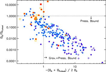
Figure 8. Comparison of terms in the virial equation, following Pattle et al. (2015). The vertical axis shows the ratio of self-gravity to pressure, i.e., the confinement ratio, showing that in most cores, pressure plays a more significant role in binding the cores than gravity does. The horizontal axis shows the ratio of energy densities with cloud pressure included. Inclusion of cloud pressure causes most of the dense cores to be bound, with the majority of that binding attributable to the weight of the overlying cloud material. See Figure 6 for the plotting conventions used.
Download figure:
Standard image High-resolution image3.3.2. Filament Pressure
As discussed in Section 2.5, cores are typically found embedded within filaments in the larger molecular cloud structure. Like the larger molecular cloud, these filaments will also help to confine the dense cores. Since it is difficult to disentangle the column density belonging to the filaments from that belonging to the dense cores with simple techniques due to their similar size scales, we instead use previous observations to estimate a lower limit to the confining pressure due to filaments. Tafalla & Hacar (2015) observed filaments and cores in the Taurus L1495/B213 region using a combination of observations of the dust continuum and of molecular emission lines. They used these observations to model the density profile of the filaments in locations where cores were not present, using a cross-sectional profile of

where n is the density at radial separation r, n0 is the central density, r0 is the characteristic size, and α is the power-law dependence (Whitworth & Ward-Thompson 2001). Across eight different filaments in Taurus, Tafalla & Hacar (2015) find  cm−3,
cm−3,  (at an assumed distance of 140 pc), and
  , while a characteristic temperature of 10 K was assumed.
The pressure induced by the weight of overlying material in an isothermal filament can be expressed as

(see Appendix C), where  is the column density through the center of the filament. The binding pressure on cores from the filaments measured in Taurus can therefore be estimated using the model estimates of Tafalla & Hacar (2015). Filaments in Orion, however, are likely to be much more dense than those found in Taurus, and therefore the Taurus estimate provides us with a lower limit to the true filament pressure. Generally, the pressure exerted by the cloud on cores is about a factor of 10 higher than the pressure exerted by these model filaments. Figure 9 shows the resulting energy density ratios with this additional pressure included (see also the following section for a further pressure term added).
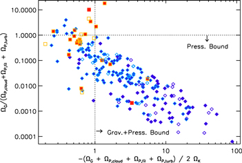
Figure 9. Comparison of terms in the virial equation, similar to that shown in Figure 8. Here,  includes the pressure of the cloud weight, the pressure of the filament weight, and the turbulent pressure. See Figure 6 for the plotting conventions used.
Download figure:
Standard image High-resolution image3.3.3. Turbulent Pressure
In addition to the weight of overlying material, turbulent pressure, i.e., pressure induced from the material of higher velocity dispersion and lower column density surrounding the cores, may also be present. We estimate the magnitude of this pressure in an approximate way. Shimajiri et al. (2014) obtained 13CO (1−0) and C18O (1−0) observations of the northern portion of Orion A, extending slightly southward of the main ISF. According to their Figure 2, the C18O (1−0) emission has a velocity dispersion <1.5 km s−1 everywhere, with most of the gas having velocity dispersions <0.75 km s−1. They assume a mean density of material traced by C18O (1−0) emission of 5 × 103 cm−3, based on previous analysis by Ikeda & Kitamura (2009). Using these estimates, the turbulent pressure on the dense cores can be written as

(e.g., Pattle et al. 2015). A more careful measurement of both the mean gas density and typical CO velocity dispersion around each dense core (or even the velocity dispersion of the surrounding fainter NH3 emission) would be required to obtain a more precise estimate of the turbulent confining pressure. Nonetheless, using the present equation to approximate the influence of turbulent pressure in combination with the pressure of the filament weight discussed above, Figure 9 shows that all cores have slightly increased energy density ratios, with an additional six dense cores now appearing to be bound. We emphasize that more precise, core-specific, estimates for both the turbulent pressure and the pressure of the filament weight could yield additional binding, especially as the latter pressure estimate is a lower limit.
3.3.4. Bonnor–Ebert Sphere Pressure
Cores are often approximated as Bonnor–Ebert (BE) spheres (Ebert 1955; Bonnor 1956), a spherically symmetric, isothermal equilibrium model where self-gravity and an external binding pressure balance internal thermal motions. In this model, the maximum external binding pressure for a stable BE sphere model can be expressed as
(Hartmann 1998). While we do not find any correlation between the critical binding pressure of a BE sphere and the estimated pressure on each core from the weight of the overlying cloud material, the values span a similar range. The mean and standard deviation of  is 6.5 ± 0.8 (where PBE,crit/kB is in K cm−3). This rough similarity in pressures between the BE sphere model and those estimated from the weight of the cloud suggests that the BE sphere model may provide a reasonable representation of the cores, although this conjecture should be tested more carefully through measurements of the radial column density profile of the cores.
3.4. Concentration
When only information on the dust continuum is available for cores, their stability is often assessed in terms of their concentration, or peakiness. Following Johnstone et al. (2001), the concentration, C, can be written as
where B is the telescope beam size, Stot is the total flux observed, and Fpk is the peak flux density observed. Typically, B is expressed in arcsec, Stot in Jy, R in arcsec, and Fpk in Jy beam−1. In the BE sphere model, the minimum concentration is 0.33 when observed in 2D, representing a sphere of uniform density, while the maximum concentration for a stable configuration is 0.72 (Johnstone et al. 2000). In Figure 10, we show the concentration measured for each dense core compared to its respective energy density ratio. Cores of higher concentration have more mass within a smaller size, and therefore would be expected to have stronger self-gravity, and hence a higher energy density ratio. As plotted in Figure 10, there is an absence of low-concentration, strongly bound cores and high-concentration, strongly unbound cores, both of which represent states that would be difficult to populate or maintain. There is no further correlation visible between the two quantities.
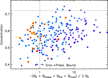
Figure 10. Comparison of the central concentration of the dense cores with their energy density ratio as shown in Figure 8. The horizontal dotted line marks the maximum stable concentration for the BE sphere model, while the vertical dotted line denotes the boundary between bound (right) and unbound (left) systems. Note that very few of the dense cores have concentrations exceeding that expected for a stable Bonnor–Ebert sphere model. See Figure 5 for the plotting conventions used.
Download figure:
Standard image High-resolution imageSome of the protostellar cores have low concentration values. Previous studies, such as van Kempen et al. (2009), have found low-concentration protostellar cores when the core evolution is more advanced, i.e., much of the core material has already been accreted onto the central protostar or dispersed by protostellar outflows, making the remaining envelope traced by the submillimeter continuum observations appear more diffuse. Angular resolution and the core identification algorithm used also play a role in the concentrations observed, since both of these influence the peak and total flux associated with each core.
3.5. Regional Variation
We additionally checked whether or not there are any bulk differences in the virial properties of dense cores associated with the ISF and the remainder of the field. Lane et al. (2016) identified clusters of dense cores across Orion A using minimal spanning trees. One of these clusters roughly encompasses the ISF, and therefore provides a simple way to identify dense cores either associated or not associated with the ISF. In all of the previous figures showing the properties of dense cores, filled symbols denote cores associated with the ISF, while open symbols show cores not associated with the ISF. Dense cores associated with the ISF tend to have slightly smaller energy density ratios than the remaining cores, due to their typically smaller sizes and therefore much smaller  values, but the two populations largely overlap. The starless cores in the ISF have typical energy density ratios of
  , while the starless cores outside the ISF have typical values of 0.62 ± 0.42 (median and median absolute deviation quoted for both). The non-ISF population that we analyze is small at present (39 starless cores), but the full GAS map of Orion A will extend much further south than the DR1 map analyzed here, and will allow for a more stringent test of whether or not virial properties vary between the ISF and the rest of Orion A.
3.6. Comparison to Li et al. (2013)
As noted in Section 3.2, Li et al. (2013) observed NH3 in cores in the OMC2 and OMC3 regions of Orion A and assessed their virial nature. While Li et al. (2013) also find that many of their dense cores are not self-gravitating ( ), they do not report virial ratios as high as those found in our analysis. The relative lack of high virial ratios in Li et al. (2013) can be attributed to our greater sensitivity to lower mass cores. For example, almost none of the cores of Li et al. (2013) have masses below 1
  , while more than half of our cores (65%) do. As discussed earlier, higher-mass cores tend to be more self-gravitating, so it is reasonable that the lower mass cores in our sample have larger virial ratios than those reported in Li et al. (2013).
In their full virial analysis, Li et al. (2013) include a turbulent pressure term estimated assuming a mean gas density of 104 cm−3 and a mean velocity dispersion of 1 km s−1. This implies a slightly larger turbulent pressure than the one we estimate in Section 3.3.3, which we noted is typically smaller than the pressure binding provided by the overlying cloud material that we estimated for each core individually. Li et al. (2013) also include a magnetic support term in their analysis, assuming a typical field strength of 0.1 mG based on nearby observations of the Zeeman effect in CN. Including both the turbulent pressure binding and magnetic support reduces the number of supervirial cores in their analysis, although nearly half (47%) of their cores still appear to be unbound, with a "critical mass ratio" above one. The overall conclusions of Li et al. (2013) therefore seem consistent with our own results, given the different core samples and different assumptions used for the virial analysis.
New results from the BISTRO survey (Ward-Thompson et al. 2017) suggest that the total magnetic field strength may be substantially larger than assumed in the analysis of Li et al. (2013). Using the Chandrasekhar–Fermi method (Chandrasekhar & Fermi 1953), Pattle et al. (2017b) estimate a magnetic field strength in the OMC-1 region, i.e., the central densest portion of the ISF) to be 6.6 ± 4.4 mG in the plane of the sky. At this level, the magnetic field would contribute significantly to the energy density of each core. Inclusion of the magnetic pressure would serve to increase the amount of internal support against the gravitational collapse of the cores, thus points in Figure 9 would move up and to the left. The magnetic pressure may not be well approximated by a constant field strength value over the large area of Orion A included in our analysis, because the field strength derived only for the densest part of the cloud may not be representative of the entire region. Therefore, while we exclude the magnetic support term from our virial analysis, we note that this should be revisited when estimates of magnetic field strength are available for a larger extent of Orion A.
4. Discussion
The potential for dense cores to be pressure-bound due to the weight of the overlying molecular cloud material has been considered for several decades (e.g., Elmegreen 1989; Bertoldi & McKee 1992), and some early observations supported this hypothesis (e.g., Keto & Myers 1986). Other types of external pressure have also been considered, including intercore ram pressure (Miettinen et al. 2010), ram pressure generated by core accretion (Naranjo-Romero et al. 2015; Seo et al. 2015), radiation pressure (Seo & Youdin 2016), and turbulent shocks (Gong & Ostriker 2015). A related issue is the role of tidal forces within molecular clouds. As discussed in Ballesteros-Paredes et al. (2009), tidal disruption should be considered for a full virial analysis of molecular clouds. On the scale of cores, however, tidal compression is more likely than tidal disruption, and is generally expected to contribute less than self-gravity for smaller cores. We therefore expect tidal effects to increase slightly the total number of bound cores in our sample. Beyond the role of external pressure, whether dense cores are in stable equilibrium, unstable equilibrium (e.g., Field et al. 2011), or not in equilibrium at all, as suggested by some numerical simulations (e.g., Ballesteros-Paredes et al. 2003; Naranjo-Romero et al. 2015), is an additional issue to consider. Our analysis makes the simplest and usual assumption that the dense cores evolve sufficiently slowly that the parameters of the virial equation measured provide a reasonable approximation of the full virial state of the cores.
On the kinematic side, we made the simple assumption that the entire velocity dispersion of the core acts to provide internal thermal plus non-thermal pressure support. While this assumption is reasonable for the thermal pressure, the non-thermal velocity dispersion almost certainly does not represent only isotropic small-scale motions that provide additional pressure support. For example, some of the non-thermal velocity dispersion could be caused by infall motions within the core, which can lead to broader emission lines in dense gas tracers (e.g., Myers 2005; Bailey et al. 2015). For the protostellar cores, where we know that infall motions must be present, in addition to some of the starless cores where infall has begun but has not yet produced a detectable central protostar, the observed line widths will be larger due to infall motion (e.g., Caselli et al. 2002). Our present analysis therefore overestimates the amount of internal pressure support, and hence underestimates the level of binding of these cores. Mapping or pointed observations of a reliable infall tracer such as HCN (e.g., Sohn et al. 2007) could be used to help remove this bias in our analysis.
A final subtle consideration is the degree to which the column density and velocity measurements we use correspond to single discrete cores in three-dimensional space. Beaumont et al. (2013) ran a careful comparison of numerical simulations of a molecular cloud as viewed in true 3D (position–position–position, or PPP) space versus the view inferred from synthetic 13CO (1−0) observations of the position–position–velocity (or PPV) structures. They found that the lack of perfect correlation between PPP and PPV structures led to scatter in the virial parameters by a factor of about two. Since NH3 traces denser gas than 13CO, the correspondence between structures is likely moderately better, because line-of-sight confusion is expected to play a smaller role in dense gas, which has a lower volume filling fraction. Nevertheless, the high average density of Orion A allows for the possibility that some of the apparent cores in our SCUBA-2 based catalog could be chance alignments of somewhat dense gas along the line of sight rather than representing a true core or could include some contamination from the material surrounding a true core. Since our analysis requires not only NH3 (1, 1) but also NH3 (2, 2) emission for cores to be reasonably well detected (at S/N > 3), we expect that there should be a minimal number of unreal cores in our analysis, but it is possible that a few of our cores with the faintest and broadest NH3 spectra fall into this category.
4.1. Previous Studies with Pressure
Our conclusion that dense cores in Orion A are significantly bounded by the pressure of the surrounding cloud material is a result that has been found in other nearby molecular clouds as well, spanning a range of environments. One example is the nearby Pipe Nebula, a star-forming environment significantly different from Orion A. Dense cores in the Pipe have typical volume densities of less than 104 cm−3, sizes of ∼0.2 pc, non-thermal velocity dispersions of ∼0.2 km s−1, and inhabit a cloud with a mean extinction of  mag and a total mass of
 that is located a mere 130 pc away (Alves et al. 2007; Lada et al. 2008, and references therein). Lada et al. (2008) used pointed NH3 or C18O observations, in combination with dense core sizes and masses estimated using extinction mapping, to demonstrate that most dense cores in the Pipe have insufficient mass to be gravitationally bound. Furthermore, the vast majority of the internal pressure support in Pipe cores was found to be from thermal pressure rather than non-thermal motions. They also found a surprising similarity in the total internal pressures of Pipe cores across the cloud and argued that the most likely source of pressure on Pipe core boundaries is that caused by the weight of the overlying cloud material. Indeed, typical internal core pressures tend to be slightly larger in the "bowl" of the Pipe than in the 'stem'; the former area is also associated with higher mean cloud column densities. Magnetic pressure may also play an important role in confining cores in the Pipe, as argued by Alves et al. (2008). In contrast to the Pipe, Orion A has a mean cloud column density contributing to the cloud external pressure that is much higher (a factor of >5), and non-thermal motions and perhaps additional sub-core bulk motions provide significant contributions to the internal pressures of its dense cores.
Several other studies examining the role of cloud pressure have been performed in star-forming regions that have properties intermediate to the Pipe and Orion A (i.e., cloud mass, volume density of dense cores, size, and non-thermal velocity dispersion). In the Ophiuchus molecular cloud, three independent analyses using different data sets all came to the conclusion that external cloud pressure is important in confining many cores in the cloud. Specifically, Johnstone et al. (2000) argued this point based on Bonnor–Ebert sphere modeling of dust continuum observations at 850 μm and the level of pressure expected from ambient cloud material, Maruta et al. (2010) used Nobeyama H13CO+ observations, while Pattle et al. (2015) used a combination of SCUBA-2 850 μm dust continuum data and IRAM 30 m N2H+ and C18O observations. In the Perseus molecular cloud, Kirk et al. (2007) analyzed the dense cores, while Sadavoy et al. (2015) analyzed the larger B1-E structure, both also finding evidence that pressure confinement is important. Note, however, that Foster et al. (2009) also analyzed dense cores in Perseus and found instead that self-gravity alone was sufficient to confine them. This difference is primarily due to the larger masses derived for the dense cores by Foster et al. (2009) using CSO Bolocam data, rather than higher resolution JCMT SCUBA data of Kirk et al. (2007). Foster et al. (2009) furthermore did not estimate the magnitude of cloud pressure to see how it compares with core self-gravity, and it is likely that such an estimate would provide a larger amount of binding than they estimated from self-gravity alone. In the Taurus L1495/B218 region, Seo et al. (2015) analyzed the virial properties of filaments and smaller structures using NH3 observations, and found that most of the small NH3 structures are gravitationally unbound when considering just the balance between self-gravity and thermal plus non-thermal support. They argued that many of these structures, especially the youngest ones, appear to be pressure-confined, and that cloud pressure is a reasonable candidate for the source of that pressure, with ram pressure from material inflowing to the system being their other main candidate. In the Cepheus clouds, Pattle et al. (2017a) performed a virial analysis using a combination of JCMT SCUBA-2 850 μm dust continuum and archival 13CO observations to argue that cloud pressure is required to bind most of the dense cores. Similarly, Kirk et al. (2016) find suggestive evidence that cloud pressure is important for dense cores in Orion B, although there, the analysis lacks kinematic information to provide precise estimates of the dense cores' temperatures and non-thermal motions.19
For more distant (non-Gould Belt) star-forming regions, Kauffmann et al. (2013) performed a self-consistent virial analysis combining observations from a variety of previous surveys. While external pressure was not included in their analysis, a comparison of self-gravity and non-thermal motions showed that the majority of structures were unbound. Structures that were bound were either much larger entities (masses above 100  ) or were in regions of high-mass star formation, or both. Kauffmann et al. (2013) speculate that the structures, which do appear to be gravitationally unbound, may in fact be pressure-bound. Additionally, Barnes et al. (2016) analyze a large sample of massive molecular clumps observed with the CHaMP survey in HCO+ and 12CO emission to demonstrate that the less dense gas traced by 12CO appears to provide significant pressure binding to the more compact clumps traced by HCO+, at a sufficient level that most of the clumps are near virial equilibrium. Thus, while it may be the case that high-mass stars form under a different mode, dense cores that form low- to intermediate- mass stars appear to be well represented by a large virial parameter, requiring the presence of some additional factor such as external pressure to remain bound.
Some numerical simulations have also illustrated the importance of cloud pressure to the formation and evolution of dense cores. Lucas et al. (2017) show that, for otherwise identical simulations of star-forming regions, either the absence of a cloud envelope at the beginning of formation, or the removal of such an envelope during evolution, leads to less dense substructure forming and to markedly lower star formation efficiencies.
Despite the differences in the analyses described above, it is striking that all of these studies come to a similar conclusion: pressure from the ambient cloud material on dense cores is important and often is required to keep the cores bound. The fact that this conclusion holds across such different star-forming environments from analyses using different techniques suggests that this phenomenon is a universal feature of star formation.
The one major component missing from most virial analyses of core populations is the support provided by magnetic fields. The magnetic field strength remains challenging to observe directly, although estimates can be made based on the field alignment, as measured by polarization data. Polarization observations are beginning to be available over larger areas of molecular clouds at lower resolution through telescopes such as Planck (e.g., Planck Collaboration et al. 2015) and Blast-Pol (e.g., Fissel et al. 2016), and at higher resolution with the JCMT's POL-2 (through the BISTRO survey; Pattle et al. 2017b; Ward-Thompson et al. 2017).
5. Conclusion
We perform a simple virial analysis of the dense cores in Orion A and find that most of them are bound. We likely underestimate the true number that are bound, since our estimate of the binding pressure from the weight of filaments surrounding the dense cores is a lower limit to the true value. The majority of the dense core binding comes in the form of pressure, mostly from the weight of the ambient cloud material rather than self-gravity or other forms of binding pressure. Qualitatively, the picture that the pressure from surrounding molecular cloud material is important, or essential, to keeping dense cores bound appears common to a variety of local molecular cloud environments. Thanks to the efforts of a variety of recent surveys of nearby molecular clouds, there are high-quality, large-area maps available to allow for a uniform assessment of the sizes and masses of dense cores (e.g., the JCMT and Herschel Gould Belt Surveys; Ward-Thompson et al. 2007b; André et al. 2010), their protostellar content (e.g., the Spitzer c2d and Gould Belt Surveys and the Herschel Gould Belt Survey, Harvey et al. 2008; Evans et al. 2009; André et al. 2010), and ambient cloud material (e.g., using variants on the near-infrared color excess, or NICE technique; Lombardi & Alves 2001). The Green Bank Ammonia Survey (Friesen et al. 2017) provides the necessary components to perform the type of virial analysis presented here, measuring both the temperatures and internal velocities of dense gas associated with the cores. The results of a similar virial analysis performed across all of the molecular clouds mapped by GAS should provide an answer to the question of whether or not the pressure of molecular cloud material is indeed an essential component to (local) star formation.
R.K.F. is a Dunlap Fellow at the Dunlap Institute for Astronomy & Astrophysics. The Dunlap Institute is funded through an endowment established by the David Dunlap family and the University of Toronto. J.E.P., P.C., A.C.T., and A.P. acknowledge the financial support of the European Research Council (ERC; project PALs 320620). E.W.R., C.D.M., and J.DiF. are supported by Discovery Grants from NSERC of Canada. The National Radio Astronomy Observatory is a facility of the National Science Foundation operated under cooperative agreement by Associated Universities, Inc. S.S.R.O. is supported by NSF grant AST-1510021. The JCMT has historically been operated by the Joint Astronomy Centre on behalf of the Science and Technology Facilities Council of the United Kingdom, the National Research Council of Canada, and the Netherlands Organisation for Scientific Research. Additional funds for the construction of SCUBA-2 were provided by the Canada Foundation for Innovation. The identification number for the program under which the SCUBA-2 data are used in this paper is MJLSG41. This research made use of Astropy, a community-developed core Python package for Astronomy (Astropy Collaboration et al. 2013). Figures in this paper were creating using the NASA IDL astronomy library (Landsman 1993) and the Coyote IDL library (http://www.idlcoyote.com/index.html).
Facilities: Green Bank Telescope - , JCMT (SCUBA-2) - .
Software: Astropy (Astropy Collaboration et al. 2013), Starlink (Currie et al. 2014), atrous.pro (https://github.com/low-sky/idl-low-sky/tree/master/wavelet).
Appendix A: Core Catalogs
Defining dense cores is generally challenging (e.g., Pineda et al. 2009) and is especially difficult in Orion A due to the high level of larger-scale structure present along the ISF. To test whether or not our conclusions are robust against uncertainties in the definitions of dense cores, we reran our analysis using two independently derived core catalogs: the FellWalker-based catalog from Lane et al. (2016) and a Hessian-based core identification algorithm presented and adopted in Salji et al. (2015). Both of these catalogs are based on the JCMT GBS SCUBA-2 850 μm data observations of Orion A, similar to the getsources-based catalog of Lane et al. (2016) used for our main analysis. Below, we describe each of these catalogs in detail and present a virial analysis based on each. We note that we do not include a similar analysis for the structure catalogs presented in Mairs et al. (2016), because that analysis does not extend far enough north in Orion A to match the GAS coverage.
A.1. FellWalker Catalog of Lane et al.
As discussed in Section 2.2, Lane et al. (2016) presented two dense core catalogs for Orion A, one using getsources, which we adopted for our main analysis, and also one using FellWalker, which we examine here. FellWalker identifies peaks based on local gradients, effectively associating any pixel lying along an upward path to a peak with that peak. There is no assumed shape for each core, and each pixel can be assigned to a maximum of one peak. When calculating the NH3-based properties of each core, analogously to Section 2.4, we use the full core footprint. Otherwise, we follow an identical procedure to that presented for the getsources-based dense core catalog.
In Figure 11, we show the results from the virial analysis using instead the FellWalker dense core catalog. As in our main analysis, we see that nearly all of the dense cores are bound (energy density ratios greater than one). Only seven of the cores have sufficient self-gravity to be entirely bound without the pressure of the cloud (i.e.,  ), so our conclusion that pressure binding is required for the majority of dense cores holds.

Figure 11. Comparison of the energy density ratio and confinement ratio for dense cores identified using FellWalker by Lane et al. (2016) (left panel) and by Salji et al. (2015) using a self-developed method (right panel). See Figure 6 for the plotting conventions used. Note that the right panel follows a different color convention than previous figures: blue points show starless cores, while red points show prestellar cores. Protostellar cores were eliminated from the catalog of Salji et al. (2015) and not published.
Download figure:
Standard image High-resolution imageA.2. Catalog of Salji et al.
Salji et al. (2015) analyzed the region around the ISF in Orion A using an early JCMT GBS data release that did not reach the final survey depth and an early reduction method that is less sensitive to larger-scale structure in the cloud ("Internal Release 1"). To identify dense cores, Salji et al. (2015) developed a new structure detection algorithm, tuned to identify only compact and roughly round sources. Sources identified with protostars were also removed from their final published catalog. The remaining cores were classified as either starless or prestellar based on a thermal stability analysis using only SCUBA-2 data (and no kinematic information). To derive the NH3-based properties for each core, we follow a similar procedure to that in the main analysis: we consider all pixels within the 1σ contour of the peak core position. Since Salji et al. (2015) did not publish axial ratios of dense core or a rotation angle, we assume the cores are well described by a single radius.
The right panel of Figure 11 shows the virial analysis for the dense cores of Salji et al. (2015). Here, the cores appear to follow a much more linear trend, suggesting that higher self-gravity and higher cloud pressure values tend to go together. The distinction that Salji et al. (2015) made between starless and prestellar cores does appear to be largely borne out in our virial analysis, with the prestellar cores tending to lie higher (more bound by both self-gravity and cloud pressure) than the starless cores. Although the qualitative appearance of the plot differs dramatically from our main analysis, we find that our main conclusion still holds: the majority of dense cores are bound (94%), and none would appear to be bound if the pressure from the cloud were ignored.
Appendix B: Estimate of Cloud Pressure
As discussed in Section 2.5, one complication in estimating the external cloud pressure is determining whether gas on different scales is associated with the core or the cloud. Attributing all of the material observed to cloud-wide material would lead us to overestimate the level of pressure exerted on the cores. In our main analysis, we filtered the map of column density of Lombardi et al. (2014) to trace only structures on ∼0.5 pc scales and larger. Here, we examine the impact of that choice of scale on our final results. We note that our test of the choice of scale also indirectly tests the choice of method for measuring the large-scale column density. The variation between methods at a single spatial scale is likely to be much smaller than the variation induced by significant changes to the scale adopted.
The à Trous algorithm we apply for filtering can be applied on length scales of  pixels. For context, 0.48 pc corresponds to 16 pixels in the original map of Lombardi et al. (2014). In Figure 12, we show a comparable analysis to that in Figure 8 but with the cloud pressure calculated instead from a map of column density filtered to 0.24 pc (8 pixels) and 0.97 pc (32 pixels). Although points do shift for each of the different choices of column density, minimal changes to the distribution of energy density ratio above or below one occur.

Figure 12. Examining the effect of different smoothing scales on the cloud pressure derived for each core. The left panel shows the cloud pressure derived including the cloud column density up to scales a factor of two smaller than the nominal value (i.e., roughly 0.25 pc). The right panel shows the cloud pressure derived including the cloud column density up to scales a factor of two larger than the nominal value (i.e., 1 pc). There is only a minimal shift in the points compared to Figure 8; in both cases, nearly all cores remain sub-virial and pressure-bound. See Figure 6 for the plotting conventions used.
Download figure:
Standard image High-resolution imageIn Figure 13, we examine the most extreme cases, comparing the results if instead the full, unfiltered map of column density or an extremely filtered map (7.7 pc or 256 pixels) were used. In the case of no filtering, we again see that most of the cores have energy density ratios above one. Only in the extremely filtered map do we find that the majority of cores are unbound. In other words, a significant amount of cloud material must be excluded from our estimate of cloud pressure for most of the dense cores to be not pressure-confined.
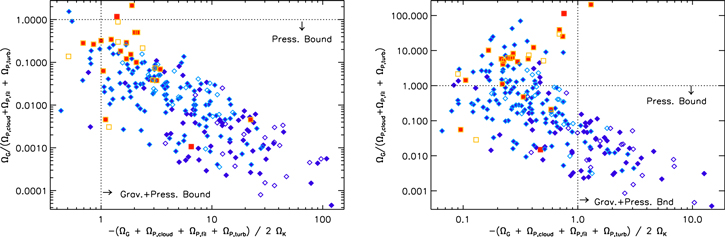
Figure 13. Examining the effect of different smoothing scales on the cloud pressure derived for each core. The left panel shows the cloud pressure derived using the total cloud column density measured, i.e., with no filtering applied. The right panel shows the cloud pressure derived including only the maximum smoothing scale for the cloud column density, i.e., 8 pc. In the former case, nearly all dense cores are sub-virial and pressure-bound, while in the latter case, many of the cores are supervirial, while pressure continues to dominate over gravity regardless of the level of confinement on the core. See Figure 6 for the plotting conventions used.
Download figure:
Standard image High-resolution imageThese tests show that, barring an extreme allocation of core-like and cloud-like material in the column density map of Lombardi et al. (2014), we come to the same conclusion: pressure from the ambient cloud material strongly dominates over self-gravity in keeping the dense cores bound. Given the fact that the amount of cloud pressure estimated for each core varies by a significant amount (often a factor of 10 between the unfiltered and maximally filtered cases), we may also surmise that changing the overarching assumption in our method, i.e., assuming that the cloud is spherically symmetric, is also unlikely to change this conclusion, although the precise amount of pressure binding attributable to each core would vary in different models.
Appendix C: Derivation of Cloud Pressure
Here we derive a useful expression for the hydrostatic pressure on a protostellar core embedded within a larger cloud. We begin with a spherical cloud of radius  , with a density profile
  , enclosed mass
  , and mean column (or more precisely, mass surface density)
  within r. The bounding pressure is
  . From any point, the column to the surface (along a radial path) is
  . The wisdom of these definitions is that the hydrostatic relation can be rewritten entirely in terms of column density:

which can be integrated if the relation between  and
and  is known. Note also that
Suppose we adopt a power-law density profile,  , for which
  then
then  . If
. If  is the mean column of the entire cloud,
Equation (18) can then be integrated:

The pressure is related to the mean cloud column and the column to the surface; for the characteristic GMC profile k = 1, Equation (19) reduces to the expression given by McKee (1989).
Within our power-law density profile, one could also use the expression  where
where  (McKee & Tan 2003). The advantage of expression (19) is that it avoids making reference to the radius r, and is therefore more closely related to observed quantities and more robust to deviations from spherical symmetry.
It is also useful to consider non-spherical geometries such as sheets and cylinders, for which the maximum column  perpendicular to the axis (for cylinders) or along the surface normal (for sheets) is the relevant scale; this quantity is twice the maximum value of
  . For a sheet confined by a surface pressure Ps, the overpressure is
  , for which the maximum (midplane) value is
  . Within an unmagnetized isothermal filament (Stodólkiewicz 1963; Ostriker 1964), the central pressure is at least20
 .
.
When estimating the pressure on a given core, one generally does not know the values of  and
and  directly from observations, but rather the projected column
  without any indication of how much column is in the background. For this reason, we now consider how P should be inferred from the column map.
C.1. Evaluation for an Observed Core
What is the most reasonable range of pressures to associate with a specific core, given a map of the projected column Σ? A natural choice is to associate  with the mean of Σ within the cloud boundaries, and
  with one-half of Σ at the location in question, but there are several ambiguities. First, the external pressure Ps must be guessed at. Second, our Σ map may be contaminated by emission unrelated to the structure of interest. Third, if the density distribution is not isotropic, Σ is affected by inclination. Fourth, one usually does not know how much of Σ is in front of the core and hence what value to associate with
  . Finally, observations may suffer from intrinsic uncertainties involving finite resolution, spatial filtering, emission-to-mass conversions, and the like.
We concentrate on the fourth ambiguity (foreground and background). The natural assumption that half of Σ is in the foreground tends to maximize P, but it is more rigorous to adopt a model and some prior expectations regarding the occurrence of cores within clouds, and to derive a probability distribution from P. Let us assume: (i) no cores exist with  , a situation corresponding to extinction thresholds observed in various regions (Pak et al. 1998; Johnstone et al. 2004) perhaps because of far-UV photoionization (McKee 1989). (ii) The probability of finding a core scales as
  per unit volume, a scenario accommodating a constant star formation rate per unit mass (
 ) and a dynamically limited rate
  .
.
The differential cumulative probability is then  , where z is distance along the line of sight, except
  where
where  .
.
For the special case  ,
,  so the column toward the core is uniformly distributed within its allowed range. In the case of a planar sheet,
  is uniformly distributed from
  to
to  . The median pressure within this distribution is lower than the midplane value by
To go further, we require relations among P, ρ, and z Hence, we adopt here the spherical model: then  where
where  is the polytropic exponent. Also,
  if ϖ is the projected offset from the cloud center and z = 0 at the cloud center. Working out dz in terms of dP,
Note that for the dynamical star formation rate ( ) the numerator is constant and
  so long as
  .
.
The next step is to determine the maximum possible pressure by determining the maximum value of  along the line of sight, given the observed value of Σ, i.e.,
  ). Often we can ignore the cloud boundary and extend a line-of-sight integration to infinity. This assumption is especially reasonable if
  , which is usually the case for giant molecular clouds. We then obtain
The middle expression comes from integrating through an infinite sphere, and the quadratic approximation is exact for  and errs by only 0.6% over the entire range. It shows that the usual assumption (
 ) is correct when k = 1, but amounts to an overprediction in steeper density profiles.
Once  and
and  have been determined, Equation (20) provides the probability density. In Figure 14, we plot the factor relating the median overpressure to the maximum value.
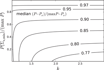
Figure 14. Median overpressure, relative to the theoretical maximum, for cores detected within spherical clouds, assuming that the probability per unit volume scales as  for columns
  to the surface, i.e., pressures
  . Theoretical maximum and minimum pressures are determined from
  and
and  (Equation (21)) via Equation (19), and the probability density follows Equation (20). This plot assumes
  .
.
Download figure:
Standard image High-resolution imageFootnotes
- 15
DR1 maps and data products are all publicly available at https://dataverse.harvard.edu/dataverse/GAS_DR1.
- 16
We note that these equations assume that there is no grain growth, a process that might affect the scaling at the highest column densities.
- 17
We use the IDL program atrous.pro developed by Erik Rosolowsky, which is available at https://github.com/low-sky/idl-low-sky/tree/master/wavelet.
- 18
A Plummer-like column density distribution has
 where Rflat is the radius of the central flat portion of the core and η describes the outer power-law slope (see Pattle 2016 for more information).
 - 19
GAS will provide NH3 observations in a future data release, however.
- 20
In our expression
neglects the column of the bounding medium, and P reaches this lower limit when the bounding pressure is effectively zero.

