


Abstract
We present high-resolution, spatially resolved, near-infrared spectroscopy and imaging of the two components of DF Tau, a young, low-mass, visual binary in the Taurus star-forming region. With these data, we provide a more precise orbital solution for the system, determine component spectral types, radial velocity, veiling and  values, and construct individual spectral energy distributions. We estimate the masses of both stars to be
  . We find markedly different circumstellar properties for DF Tau A and B: evidence for a disk, such as near-infrared excess and accretion signatures, is clearly present for the primary, while it is absent for the secondary. Additionally, the
  and rotation period measurements show that the secondary is rotating significantly more rapidly than the primary. We interpret these results in the framework of disk-locking and argue that DF Tau A is an example of disk-modulated rotation in a young system. The DF Tau system raises fundamental questions about our assumptions of universal disk formation and evolution.
Export citation and abstract BibTeX RIS
1. Introduction
The bimodal nature of rotation periods in young stars is often attributed to disk-locking, where the stellar magnetic field lines thread through and thus couple to the ionized inner disk (Li 1996). This coupling can occur as close to the star as a few to tens of stellar radii (Bouvier et al. 2007). In this manner the disk can apply a torque to the star, regulating its rotation. Disk-locking was first demonstrated in studies of the Taurus region, showing that the rotation period distribution of young stars with disks is different from the distribution of young stars without disks (Edwards et al. 1993). The rotation period distributions for stars earlier than M2 in the Orion Nebula Cluster (ONC) and Taurus star-forming region are bimodal, with peaks at ∼2 and ∼8 days. The rotation period distribution for the stars later than M2, however, has only a single peak at about 2 days, with a long tail toward longer rotation periods (Attridge & Herbst 1992; Herbst et al. 2002; Davies et al. 2014). Young stars with disks tend to have rotation periods around 5–8 days, depending on the Keplerian velocity at the radius at which the star's magnetic field couples with the disk (Koenigl 1991). Diskless young stars have a range of rotation periods from less than a day to around 15 days (Edwards et al. 1993). Thus, as a young star contracts toward the main sequence, as long as it is disk-locked, it can exchange angular momentum with the disk and preserve its rotation period. A young star that has lost its inner disk will spin up as it contracts. The final rotation rate of a star as it joins the main sequence is likely tied to the lifetime of its disk during pre-main sequence evolution.
It is crucial to determine circumstellar disk characteristics and stellar rotation properties in order to better understand the connection between circumstellar disk lifetimes, rotational evolution, and young stellar evolution in general. Multistar systems share common properties such as distance, age, metallicity, line of sight extinction, and environment and thus are of particular importance because their companions provide a control comparison. The triple system BD-21 1074, a member of the ∼21 Myr β Pictoris moving group, is an example of such a system (Messina et al. 2014). The A and B components of BD-21 1074 have roughly the same spectral type (M1.5 and M2.5, respectively) and a wide separation of almost 150 au. The B component has an additional close M5 spectral type companion with a 15 au separation. Despite sharing similar properties, the A component has a rotation period of about 9.3 days, while the B component has a rotation period of only about 5.4 days. Messina et al. (2014) suggest that the most plausible scenario leading to this outcome is that both components began with similar rotation periods, but the B component's interactions with its close companion led to rapid dissipation of its circumstellar disk, resulting in spin-up at an early point in its contraction and thus a faster final rotation period compared to the A component.
The young (∼1–2 Myr) visual binary DF Tau (Herbig & Bell 1988; Chen et al. 1990; Schaefer et al. 2014) in the Taurus star-forming region is a useful laboratory to examine the effects of star–disk evolution, and potentially, star–disk interactions. DF Tau comprises two equal-mass components (Section 3.2) with an angular separation of ∼100 mas, corresponding to 14 au at the assumed 140 pc distance to Taurus (Kenyon et al. 1994). Intriguingly, even though the components are of similar mass and presumably coeval, their circumstellar properties are distinct. Our observations of the primary show strong accretion signatures and a long-wavelength excess, indicative of the presence of a disk, while accretion and disk indicators for the secondary are weak and/or absent. We present new near-infrared spectroscopy and imaging of the individual stars in DF Tau (Section 2). With these data we determine the spectral types, veiling,  , radial velocity (RV), disk, and rotational properties for each component and improve the orbital parameters for the system (Section 3). Finally, we discuss DF Tau as an example of divergent circumstellar disk evolution and speculate as to the driving processes behind heterogeneous disk formation, evolution, and dissipation (Section 4). A summary appears in Section 5.
2. Observations and Data Reduction
2.1. Resolved Infrared Spectroscopy of the DF Tau Components
Spatially resolved spectroscopic observations of the DF Tau components were obtained using NIRSPEC (McLean et al. 1998, 2000) behind the adaptive optics (AO) system (NIRSPAO) on the Keck II 10 m telescope on the UT dates of 2009 December 06, 2010 December 12, and 2013 December 22 (Table 1). The 2 pixel slit for NIRSPAO is  , producing spectra with a resolution of ∼30,000 in order 49 (central wavelength 1.556 μm). This order is advantageous because of its lack of telluric absorption lines and abundance of photospheric atomic and molecular lines (Mace et al. 2012). For each observation, dark frames, flat-field frames, and Ne, Ar, Xe, and Kr comparison-lamp frames were obtained to correct for dark current and non-uniform pixel-to-pixel detector response and for wavelength calibration. Target observations were made with an AB or ABBA nodding pattern at two locations along the slit. The integration time for each nod was 300 s.
Table 1. Keck NIRSPEC Observations of DF Tau
| Date | AOa |
|---|---|
| 2009 Dec 06 | Y |
| 2010 Dec 12 | Y |
| 2013 Dec 22 | Y |
| 2001 Dec 31 | N |
| 2002 Feb 5 | N |
| 2002 Jul 18 | N |
| 2002 Oct 30 | N |
| 2002 Dec 14 | N |
Note.
aAO observations are denoted with Y, and non-AO observations are denoted with N.Download table as: ASCIITypeset image
Reductions were accomplished with the REDSPEC (Kim et al. 2015) package. REDSPEC contains routines for the spatial rectification, wavelength calibration, removal of detector, atmospheric and optical path artifacts, and extraction of spectra. The two-dimensional spectra were rectified in spatial and spectral dimensions using third-order and second-order polynomials, respectively. The spectral traces were then fit to the comparison-lamp emission lines to determine the wavelength solution. Any instrumental fringing and bad pixels were removed. For each pixel in the dispersion direction, two Gaussians were fit to the spatial point-spread function of the overlapping spectra in the cross-dispersion direction to extract the individual component spectra. Further details are provided in Schaefer et al. (2012). The normalized, barycentric-corrected spectra appear in Figure 1.

Figure 1. Angularly resolved NIRSPAO spectra of DF Tau A (top) and B (bottom). Much broader absorption lines are apparent in DF Tau B.
Download figure:
Standard image High-resolution image2.2. Unresolved Infrared Spectroscopy of the DF Tau System
Unresolved spectroscopic observations of DF Tau were obtained using NIRSPEC without AO on the Keck II 10 m telescope on the UT dates of 2001 December 31, 2002 February 05, 2002 July 18, 2002 October 30 and 2002 December 14, (Figure 2, Table 1). The 2-pixel slit was  , yielding a resolution of ∼30,000 (Mace et al. 2009). Integration times ranged from 120 to 300 s. The observing procedure and reduction process were similar to those for the resolved spectroscopy, except the OH night-sky emission lines inherent in the spectra were used for wavelength calibration (Rousselot et al. 2000).
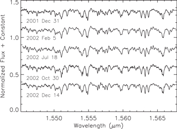
Figure 2. Angularly unresolved NIRSPEC spectra of the DF Tau system.
Download figure:
Standard image High-resolution image2.3. Resolved Infrared Imaging of the DF Tau Components
Spatially resolved imaging of DF Tau was obtained with the NIRC2 camera behind the AO system on the Keck II telescope (Wizinowich et al. 2000) on UT 2015 January 1 and 2016 October 20. On each night we obtained 6–12 dithered images in the Hcont and Kcont filters. We used the same data reduction and analysis methods described in Schaefer et al. (2014). Observations of the single star DN Tau, obtained with the same AO frame rate immediately after DF Tau, were used as a point-spread function reference to model the binary position. For the data from 2015, we corrected the positions measured for DF Tau A, B using the geometric distortion solution determined by Yelda et al. (2010). Following the realignment of the AO system and the NIRC2 camera on 2015 April 13, we used the revised distortion solution determined by Service et al. (2016) to correct the position measured in 2016. Table 2 lists the separation (ρ), position angle (PA) east of north, and flux ratio measured for DF Tau A, B.
Table 2. Keck NIRC2 Adaptive Optics Measurements of DF Tau A, B
| UT Date | Besselian Year | ρ(mas) | P.A.(°) | Filter | Flux Ratio |
|---|---|---|---|---|---|
| 2015 Jan 01 06:52 | 2015.0017 | 93.39 ± 2.24 | 195.20 ± 1.37 | Hcont | 0.791 ± 0.034 |
| Kcont | 0.520 ± 0.022 | ||||
| 2016 Oct 20 13:20 | 2016.8028 | 85.89 ± 0.41 | 182.67 ± 0.27 | Hcont | 0.797 ± 0.027 |
| Kcont | 0.545 ± 0.014 |
Download table as: ASCIITypeset image
2.4. Unresolved Photometry of the DF Tau System
We acquired unresolved BVI photometry of DF Tau using the Lowell Observatory 0.8 m f/8 telescope in robotic mode. The CCD camera provides a  field at an image-scale of
  /pixel. The system was observed 134 times on 35 nights spread out over 4 months between 2015 November 1 and 2016 February 28 UT (Table 3 and Figure 3). The field was visited up to five times each night. Exposures were 180, 60, and 20 s in the B, V, and I filters, respectively. We used the commercial software Canopus (version 10.4.0.6) to perform standard photometric reductions, with bias and flat-field correction followed by ordinary differential aperture photometry. Apertures were typically
  in diameter, depending on nightly image quality. We adopted BVI magnitudes for three comparison stars, TYC 1820-0176-1, GSC 1820-0482, and GSC 1820-0950, from the wide-field photometric surveys ASAS-3 (Pojmanski 1997), TASS MkIV (Droege et al. 2006), and APASS DR9 (Henden et al. 2016, VizieR item II/336). These adjust the photometric zero-points close to the standard system. Because of the emission-line nature of the DF Tau spectrum, there were inevitably small zero-point shifts resulting from the interplay of the DF Tau spectrum, the colors of the comparison stars, and the passband of the filters +CCD system. Our magnitudes are similar to long-term means in the three filters.
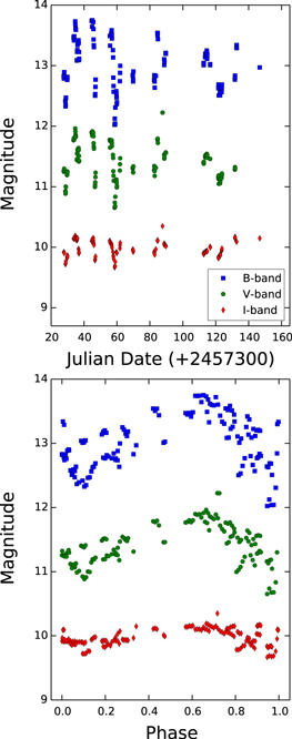
Figure 3. Top: time-series photometry in the B-band (squares), V-band (circles), and I-band (diamonds) for the DF Tau system. The errors are comparable to the size of the plot symbols. A total of 134 observations were taken over 119 days. The V-band photometry has been shifted by −0.5 mag for clarity. Bottom: phase-folded light curves with a period of 10.5 days.
Download figure:
Standard image High-resolution imageTable 3. Unresolved Photometry of DF Tau—Lowell 0.8 m
| Date | B | V | I |
|---|---|---|---|
| 2457327.67126 | 12.823 ± 0.004 | 11.757 ± 0.004 | 9.918 ± 0.004 |
| 2457327.75831 | 12.787 ± 0.005 | 11.745 ± 0.004 | 9.91 ± 0.004 |
| 2457327.84248 | 12.826 ± 0.005 | 11.769 ± 0.004 | 9.915 ± 0.004 |
| 2457327.92899 | 12.885 ± 0.005 | 11.797 ± 0.004 | 9.916 ± 0.004 |
| 2457328.0146 | 12.893 ± 0.006 | 11.797 ± 0.004 | 9.902 ± 0.004 |
| 2457328.66817 | 12.418 ± 0.004 | 11.426 ± 0.004 | 9.722 ± 0.004 |
| 2457328.75532 | 12.327 ± 0.004 | 11.384 ± 0.004 | 9.72 ± 0.004 |
| 2457328.83991 | 12.349 ± 0.004 | 11.413 ± 0.004 | 9.728 ± 0.004 |
| 2457328.92565 | 12.462 ± 0.004 | 11.501 ± 0.004 | 9.764 ± 0.004 |
| 2457329.01205 | 12.471 ± 0.005 | 11.495 ± 0.004 | 9.76 ± 0.004 |
| 2457329.66747 | 12.777 ± 0.004 | 11.691 ± 0.004 | 9.834 ± 0.004 |
| 2457329.75425 | 12.765 ± 0.004 | 11.695 ± 0.004 | 9.822 ± 0.004 |
| 2457329.83944 | 12.815 ± 0.004 | 11.752 ± 0.004 | 9.851 ± 0.004 |
| 2457329.92585 | 12.793 ± 0.004 | 11.742 ± 0.004 | 9.868 ± 0.004 |
| 2457333.65375 | 13.472 ± 0.005 | 12.266 ± 0.005 | 10.14 ± 0.004 |
| 2457333.74092 | 13.449 ± 0.004 | 12.275 ± 0.004 | 10.139 ± 0.004 |
| 2457333.82991 | 13.475 ± 0.004 | 12.301 ± 0.004 | 10.153 ± 0.004 |
| 2457333.91967 | 13.416 ± 0.004 | 12.271 ± 0.004 | 10.15 ± 0.004 |
| 2457334.0089 | 13.485 ± 0.005 | 12.301 ± 0.004 | 10.158 ± 0.004 |
| 2457334.65134 | 13.731 ± 0.005 | 12.463 ± 0.005 | 10.19 ± 0.005 |
| 2457334.73911 | 13.684 ± 0.004 | 12.413 ± 0.004 | 10.18 ± 0.004 |
| 2457334.83533 | 13.617 ± 0.004 | 12.36 ± 0.004 | 10.155 ± 0.004 |
| 2457334.92651 | 13.599 ± 0.004 | 12.342 ± 0.004 | 10.142 ± 0.004 |
| 2457335.01853 | 13.592 ± 0.004 | 12.321 ± 0.004 | 10.125 ± 0.004 |
| 2457335.64871 | 13.084 ± 0.005 | 11.94 ± 0.004 | 10.114 ± 0.004 |
| 2457335.7406 | 13.09 ± 0.004 | 11.96 ± 0.004 | 10.114 ± 0.004 |
| 2457335.83441 | 13.227 ± 0.004 | 12.043 ± 0.004 | 10.137 ± 0.004 |
| 2457335.93161 | 13.259 ± 0.004 | 12.059 ± 0.004 | 10.147 ± 0.004 |
| 2457336.02289 | 13.34 ± 0.004 | 12.112 ± 0.004 | 10.151 ± 0.004 |
| 2457336.64612 | 13.42 ± 0.005 | 12.14 ± 0.004 | 9.974 ± 0.004 |
| 2457336.73855 | 13.373 ± 0.004 | 12.105 ± 0.004 | 9.96 ± 0.004 |
| 2457336.84134 | 13.09 ± 0.004 | 11.915 ± 0.004 | 9.896 ± 0.004 |
| 2457336.93282 | 13.226 ± 0.004 | 12.009 ± 0.004 | 9.921 ± 0.004 |
| 2457337.0256 | 13.115 ± 0.004 | 11.931 ± 0.004 | 9.917 ± 0.004 |
| 2457344.6223 | 13.742 ± 0.007 | 12.398 ± 0.006 | 10.101 ± 0.005 |
| 2457344.72092 | 13.738 ± 0.005 | 12.388 ± 0.004 | 10.104 ± 0.004 |
| 2457344.82223 | 13.743 ± 0.006 | 12.396 ± 0.004 | 10.104 ± 0.004 |
| 2457344.91988 | 13.643 ± 0.004 | 12.344 ± 0.004 | 10.089 ± 0.004 |
| 2457345.01831 | 13.75 ± 0.005 | 12.415 ± 0.005 | 10.135 ± 0.004 |
| 2457345.61972 | 13.72 ± 0.007 | 12.39 ± 0.005 | 10.152 ± 0.004 |
| 2457345.71951 | 13.604 ± 0.005 | 12.333 ± 0.004 | 10.112 ± 0.004 |
| 2457345.82492 | 13.432 ± 0.004 | 12.219 ± 0.004 | 10.073 ± 0.004 |
| 2457345.92313 | 13.338 ± 0.004 | 12.165 ± 0.004 | 10.057 ± 0.004 |
| 2457346.02323 | 13.306 ± 0.004 | 12.127 ± 0.004 | 10.035 ± 0.004 |
| 2457346.61703 | 12.456 ± 0.006 | 11.496 ± 0.004 | 9.785 ± 0.004 |
| 2457346.71577 | 12.504 ± 0.005 | 11.528 ± 0.004 | 9.783 ± 0.004 |
| 2457346.81533 | 12.531 ± 0.004 | 11.574 ± 0.004 | 9.801 ± 0.004 |
| 2457346.91448 | 12.649 ± 0.003 | 11.658 ± 0.004 | 9.842 ± 0.004 |
| 2457347.01471 | 12.769 ± 0.004 | 11.732 ± 0.004 | 9.849 ± 0.004 |
| 2457355.59285 | 13.572 ± 0.005 | 12.276 ± 0.005 | 10.107 ± 0.005 |
| 2457355.69435 | 13.491 ± 0.008 | 12.258 ± 0.005 | 10.097 ± 0.004 |
| 2457355.79447 | 13.329 ± 0.007 | 12.145 ± 0.005 | 10.073 ± 0.004 |
| 2457356.59256 | 13.545 ± 0.005 | 12.264 ± 0.005 | 10.063 ± 0.005 |
| 2457356.69574 | 13.519 ± 0.005 | 12.249 ± 0.004 | 10.054 ± 0.004 |
| 2457356.79865 | 13.584 ± 0.006 | 12.268 ± 0.005 | 10.039 ± 0.004 |
| 2457356.89896 | 13.511 ± 0.006 | 12.219 ± 0.005 | 10.019 ± 0.004 |
| 2457357.00127 | 13.448 ± 0.008 | 12.171 ± 0.005 | 9.991 ± 0.004 |
| 2457357.59080 | 13.256 ± 0.005 | 12.026 ± 0.004 | 9.923 ± 0.004 |
| 2457357.69406 | 13.136 ± 0.004 | 11.974 ± 0.004 | 9.914 ± 0.004 |
| 2457357.79854 | 12.802 ± 0.005 | 11.756 ± 0.004 | 9.863 ± 0.004 |
| 2457357.90108 | 12.663 ± 0.016 | 11.681 ± 0.006 | 9.841 ± 0.004 |
| 2457358.00196 | 12.568 ± 0.006 | 11.598 ± 0.005 | 9.806 ± 0.004 |
| 2457358.60433 | 12.024 ± 0.004 | 11.152 ± 0.004 | 9.667 ± 0.004 |
| 2457358.70563 | 12.125 ± 0.003 | 11.237 ± 0.003 | 9.689 ± 0.004 |
| 2457358.81372 | 12.037 ± 0.004 | 11.175 ± 0.003 | 9.678 ± 0.004 |
| 2457358.91711 | 12.042 ± 0.004 | 11.178 ± 0.004 | 9.687 ± 0.004 |
| 2457359.01685 | 12.308 ± 0.006 | 11.334 ± 0.004 | 9.759 ± 0.004 |
| 2457359.58335 | 12.579 ± 0.004 | 11.62 ± 0.004 | 9.919 ± 0.004 |
| 2457359.68416 | 12.543 ± 0.004 | 11.605 ± 0.004 | 9.912 ± 0.004 |
| 2457359.78826 | 12.472 ± 0.004 | 11.566 ± 0.004 | 9.916 ± 0.005 |
| 2457359.89279 | 12.365 ± 0.004 | 11.488 ± 0.004 | 9.902 ± 0.004 |
| 2457359.99871 | 12.394 ± 0.008 | 11.511 ± 0.005 | 9.905 ± 0.005 |
| 2457361.76768 | 12.742 ± 0.004 | 11.767 ± 0.004 | 9.98 ± 0.004 |
| 2457361.87068 | 12.881 ± 0.004 | 11.872 ± 0.004 | 10.033 ± 0.004 |
| 2457361.97846 | 12.998 ± 0.005 | 11.97 ± 0.004 | 10.072 ± 0.004 |
| 2457369.58058 | 12.844 ± 0.005 | 11.801 ± 0.004 | 9.953 ± 0.005 |
| 2457369.68459 | 12.831 ± 0.004 | 11.823 ± 0.004 | 9.966 ± 0.004 |
| 2457369.78873 | 12.739 ± 0.004 | 11.738 ± 0.004 | 9.943 ± 0.004 |
| 2457369.88895 | 12.759 ± 0.004 | 11.734 ± 0.004 | 9.923 ± 0.004 |
| 2457369.99081 | 12.904 ± 0.005 | 11.836 ± 0.004 | 9.949 ± 0.005 |
| 2457382.58363 | 12.767 ± 0.01 | 11.773 ± 0.006 | 9.904 ± 0.005 |
| 2457382.67534 | 12.842 ± 0.01 | 11.842 ± 0.006 | 9.928 ± 0.004 |
| 2457382.77382 | 12.763 ± 0.01 | 11.793 ± 0.006 | 9.922 ± 0.004 |
| 2457382.86531 | 12.737 ± 0.012 | 11.757 ± 0.007 | 9.92 ± 0.005 |
| 2457382.94483 | 12.635 ± 0.017 | 11.678 ± 0.009 | 9.876 ± 0.005 |
| 2457383.63448 | 12.831 ± 0.007 | 11.813 ± 0.005 | 9.967 ± 0.004 |
| 2457384.58626 | 13.542 ± 0.004 | 12.285 ± 0.004 | 10.108 ± 0.004 |
| 2457384.67919 | 13.505 ± 0.006 | 12.272 ± 0.005 | 10.117 ± 0.004 |
| 2457384.76826 | 13.541 ± 0.007 | 12.294 ± 0.008 | 10.104 ± 0.005 |
| 2457387.69381 | 14.174 ± 0.005 | 12.724 ± 0.005 | 10.349 ± 0.004 |
| 2457388.66859 | 13.107 ± 0.004 | 12.03 ± 0.004 | 10.064 ± 0.004 |
| 2457388.75527 | 13.011 ± 0.004 | 11.963 ± 0.004 | 10.039 ± 0.004 |
| 2457388.84262 | 13.075 ± 0.005 | 11.994 ± 0.004 | 10.038 ± 0.004 |
| 2457389.58699 | 13.202 ± 0.004 | 12.06 ± 0.004 | 10.03 ± 0.004 |
| 2457389.67489 | 13.211 ± 0.004 | 12.067 ± 0.004 | 10.024 ± 0.004 |
| 2457389.7614 | 13.195 ± 0.004 | 12.058 ± 0.004 | 10.015 ± 0.004 |
| 2457412.60031 | 13.039 ± 0.006 | 11.905 ± 0.005 | 9.903 ± 0.004 |
| 2457412.66851 | 13.009 ± 0.011 | 11.892 ± 0.007 | 9.899 ± 0.005 |
| 2457412.73846 | 13.017 ± 0.028 | 11.879 ± 0.014 | 9.882 ± 0.009 |
| 2457412.8097 | 13.046 ± 0.015 | 11.912 ± 0.009 | 9.899 ± 0.006 |
| 2457413.60095 | 13.139 ± 0.004 | 11.985 ± 0.004 | 9.918 ± 0.004 |
| 2457413.6699 | 13.18 ± 0.009 | 12.011 ± 0.005 | 9.924 ± 0.005 |
| 2457413.74405 | 13.201 ± 0.008 | 12.017 ± 0.005 | 9.926 ± 0.004 |
| 2457413.81856 | 13.163 ± 0.011 | 12.005 ± 0.006 | 9.922 ± 0.004 |
| 2457414.60154 | 13.249 ± 0.004 | 12.043 ± 0.004 | 9.944 ± 0.004 |
| 2457414.67171 | 13.214 ± 0.005 | 12.024 ± 0.004 | 9.934 ± 0.004 |
| 2457414.74903 | 13.153 ± 0.006 | 11.995 ± 0.004 | 9.936 ± 0.004 |
| 2457414.81857 | 13.113 ± 0.008 | 11.978 ± 0.005 | 9.934 ± 0.004 |
| 2457414.8708 | 13.184 ± 0.011 | 12.022 ± 0.006 | 9.93 ± 0.005 |
| 2457416.58683 | 13.009 ± 0.004 | 11.958 ± 0.004 | 10.01 ± 0.004 |
| 2457416.65529 | 13.025 ± 0.004 | 11.96 ± 0.004 | 9.994 ± 0.004 |
| 2457421.58973 | 12.639 ± 0.004 | 11.66 ± 0.004 | 9.837 ± 0.004 |
| 2457421.65372 | 12.627 ± 0.004 | 11.631 ± 0.004 | 9.817 ± 0.004 |
| 2457421.72434 | 12.689 ± 0.004 | 11.676 ± 0.004 | 9.837 ± 0.004 |
| 2457421.78822 | 12.684 ± 0.004 | 11.686 ± 0.004 | 9.841 ± 0.004 |
| 2457421.83549 | 12.508 ± 0.005 | 11.547 ± 0.004 | 9.83 ± 0.004 |
| 2457422.59022 | 12.578 ± 0.004 | 11.616 ± 0.004 | 9.876 ± 0.004 |
| 2457422.65345 | 12.509 ± 0.004 | 11.554 ± 0.004 | 9.857 ± 0.004 |
| 2457422.72313 | 12.592 ± 0.004 | 11.61 ± 0.004 | 9.877 ± 0.004 |
| 2457422.79149 | 12.568 ± 0.004 | 11.593 ± 0.004 | 9.868 ± 0.004 |
| 2457422.84759 | 12.637 ± 0.005 | 11.629 ± 0.004 | 9.871 ± 0.004 |
| 2457423.59081 | 12.562 ± 0.004 | 11.644 ± 0.004 | 9.941 ± 0.004 |
| 2457423.65393 | 12.627 ± 0.004 | 11.693 ± 0.004 | 9.952 ± 0.004 |
| 2457423.71345 | 12.636 ± 0.007 | 11.689 ± 0.008 | 9.974 ± 0.009 |
| 2457423.79232 | 12.688 ± 0.004 | 11.718 ± 0.004 | 9.98 ± 0.004 |
| 2457431.61145 | 12.77 ± 0.004 | 11.781 ± 0.004 | 10.154 ± 0.004 |
| 2457431.6713 | 12.788 ± 0.004 | 11.795 ± 0.004 | 10.159 ± 0.004 |
| 2457431.73252 | 12.836 ± 0.004 | 11.823 ± 0.004 | 10.172 ± 0.004 |
| 2457431.79731 | 12.804 ± 0.004 | 11.803 ± 0.004 | 10.161 ± 0.004 |
| 2457432.59556 | 13.3 ± 0.005 | 12.132 ± 0.006 | 10.097 ± 0.006 |
| 2457432.64843 | 13.335 ± 0.005 | 12.161 ± 0.004 | 10.091 ± 0.004 |
| 2457432.71807 | 13.341 ± 0.005 | 12.163 ± 0.004 | 10.093 ± 0.004 |
| 2457432.77375 | 13.289 ± 0.005 | 12.126 ± 0.004 | 10.093 ± 0.004 |
| 2457446.76601 | 12.97 ± 0.006 | 11.986 ± 0.005 | 10.148 ± 0.005 |
2.5. Observations from Literature
We compiled both resolved and unresolved photometry of DF Tau (Table 4). Resolved photometry of both components includes UBVRI magnitudes from White & Ghez (2001) and averaged JHKL magnitudes and flux ratios from Schaefer et al. (2006, 2014). The unresolved photometry includes observations from Spitzer IRAC (Luhman et al. 2006), WISE, (Cutri et al. 2012), and SCUBA (Andrews & Williams 2005).
Table 4. DF Tau Photometry from the Literature
| Wavelength | Primarya | Secondarya | Systema | Reference |
|---|---|---|---|---|
| U | 12.75 ± 0.06 | 15.06 ± 0.28 | ⋯ | White & Ghez (2001) |
| B | 13.18 ± 0.05 | 14.47 ± 0.13 | ⋯ | White & Ghez (2001) |
| V | 12.43 ± 0.06 | 13.10 ± 0.1 | ⋯ | White & Ghez (2001) |
| R | 11.53 ± 0.05 | 11.84 ± 0.06 | ⋯ | White & Ghez (2001) |
| I | 10.59 ± 0.02 | 10.61 ± 0.02 | ⋯ | White & Ghez (2001) |
| J | 8.876 ± 0.029 | 8.973 ± 0.029 | ⋯ | Schaefer et al. (2014) |
| H | 7.865 ± 0.064 | 8.175 ± 0.082 | ⋯ | Schaefer et al. (2014) |
| K | 7.176 ± 0.046 | 7.923 ± 0.082 | ⋯ | Schaefer et al. (2014) |
| L | 6.27 ± 0.15 | 7.53 ± 0.15 | ⋯ | Schaefer et al. (2014) |
| 3.6 μm | ⋯ | ⋯ | <5.84 | Luhman et al. (2006) |
| 4.5 μm | ⋯ | ⋯ | <5.37 | Luhman et al. (2006) |
| 5.8 μm | ⋯ | ⋯ | 5.01 ± 0.02 | Luhman et al. (2006) |
| 8.0 μm | ⋯ | ⋯ | 4.42 ± 0.03 | Luhman et al. (2006) |
| 3.35 μm | ⋯ | ⋯ | 5.925 ± 0.051 | Cutri et al. (2012) |
| 4.60 μm | ⋯ | ⋯ | 5.076 ± 0.027 | Cutri et al. (2012) |
| 11.56 μm | ⋯ | ⋯ | 3.822 ± 0.014 | Cutri et al. (2012) |
| 22.08 μm | ⋯ | ⋯ | 2.252 ± 0.02 | Cutri et al. (2012) |
| 850 μm | ⋯ | ⋯ | 8.8 ± 1.9b | Andrews & Williams (2005) |
| 880 μm | ⋯ | ⋯ | 9.0 ± 2.0b | Harris et al. (2012) |
| 1300 μm | ⋯ | ⋯ | <25.0b | Andrews & Williams (2005) |
Notes.
aMagnitudes unless otherwise noted. bFlux is measured in Janskys.Download table as: ASCIITypeset image
2.5.1. Resolved Fine Guidance Sensor (FGS) Photometry
Based on observations with the FGS on the Hubble Space Telescope over a decade, Schaefer et al. (2003) presented time-series V-band photometry for the individual components of DF Tau. When converting the FGS counts into calibrated magnitudes, Schaefer et al. (2003) used a B − V color of 1.6 for DF Tau. However, the authors made a clerical error in reporting the system color from the component magnitudes published in White & Ghez (2001). We have corrected the component magnitudes listed in Table 1 of Schaefer et al. (2003), using an average B − V color of 1.06, computed from the time-averaged photometry in Table 4. We also corrected a transcription error in Table 5 of Schaefer et al. (2006) that lists the FGS photomultiplier tube (PMT) counts for both components of DF Tau; the correct PMT counts are listed in our Table 5. The FGS measurements prior to 1999 were obtained with the FGS3 instrument using the PUPIL filter, which has the following photometric calibration for converting the photon counts C measured with the FGS to the V-band magnitude of the object (Holfeltz et al. 1995):

where we assumed a B − V color of 1.06, and calibration constants of  and
and  mag. Measurements after the year 1999 were obtained with the refurbished FGS1r using the F583W filter; a photometric calibration has not been published for this instrument. To calibrate the photometry on DF Tau after 1999, we assumed that the secondary, which shows a lack of variability, would have the same average magnitude before and after 1999. Therefore, we used the average magnitude of DF Tau B measured with the FGS3 to calibrate the average counts measured for this component with the FGS1r to establish the photometric zero-point. The re-calibrated FGS photometry results for the individual components of DF Tau are listed in Table 6.
Table 5. Corrected PMT Counts from Schaefer et al. (2006)
| Counts (25 ms)−1 | ||
|---|---|---|
| Date | Primary | Secondary |
| 2003 Jan 23 | 1535.51 | 417.842 |
| 2003 Nov 19 | 1249.63 | 417.742 |
Download table as: ASCIITypeset image
Table 6. Corrected FGS Component Magnitudes from Schaefer et al. (2006)
| Date | Primary | Secondary |
|---|---|---|
| 1993.734 | 13.011 ± 0.345 | 13.411 ± 0.345 |
| 1993.816 | 12.171 ± 0.345 | 13.351 ± 0.345 |
| 1994.821 | 12.951 ± 0.345 | 13.261 ± 0.345 |
| 1995.055 | 12.701 ± 0.345 | 13.401 ± 0.345 |
| 1995.572 | 12.401 ± 0.345 | 13.281 ± 0.345 |
| 1997.019 | 12.647 ± 0.345 | 13.397 ± 0.345 |
| 1997.706 | 12.831 ± 0.345 | 13.361 ± 0.345 |
| 1997.884 | 12.271 ± 0.345 | 13.381 ± 0.345 |
| 1998.164 | 11.821 ± 0.345 | 13.221 ± 0.345 |
| 1999.695 | 12.637 ± 0.36 | 13.337 ± 0.361 |
| 2000.241 | 11.576 ± 0.358 | 13.306 ± 0.361 |
| 2000.671 | 12.814 ± 0.36 | 13.334 ± 0.361 |
| 2000.695 | 12.548 ± 0.359 | 13.378 ± 0.361 |
| 2001.063 | 12.406 ± 0.359 | 13.326 ± 0.361 |
| 2001.16 | 12.919 ± 0.36 | 13.219 ± 0.361 |
| 2002.129 | 12.485 ± 0.359 | 13.315 ± 0.361 |
| 2003.061 | 12.012 ± 0.359 | 13.425 ± 0.362 |
| 2003.883 | 12.235 ± 0.359 | 13.425 ± 0.362 |
Download table as: ASCIITypeset image
3. Analysis and Results
3.1. Orbital Parameters
With the additional orbital coverage provided by the NIRC2 imaging in 2015, we improved the orbit calculation of Schaefer et al. (2014). The period (P), time of periastron passage (T), eccentricity (e), angular semimajor axis (a), inclination (i), position angle of the line of nodes (Ω), and the angle between the node and periastron (ω) were determined using the Newton–Raphson method to linearize the equations of orbital motion and minimize  . The uncertainties in all quantities were determined using the diagonal elements of the covariance matrix. The total system mass was computed from Kepler's Third Law, assuming a distance of 140 pc. The orbital parameters and their errors are presented in Table 7; the best-fit orbit is shown in Figure 4. For visual orbits, there is a 180° degeneracy between ω and Ω. From our RV measurements (Section 3.4), we can establish
  for the primary (
 for the secondary).

Figure 4. Orbit of DF Tau as mapped through nearly two decades of high-resolution imaging. The black circles are NIRC2 and FGS measurements from this paper, Simon et al. (1996), and Schaefer et al. (2003, 2006, 2014). The gray circles are from Chen et al. (1990), Ghez et al. (1995), Thiebaut et al. (1995), White & Ghez (2001), Balega et al. (2002, 2004), Shakhovskoj et al. (2006), and Balega et al. (2007). The best-fit orbit of 46.1 ± 1.9 yr is shown in blue. The dotted (red) orbits were computed by varying the orbital period by 1σ (±2.8 yr) and optimizing the remaining orbital parameters. From the visual orbit solution and the identical spectral types, we estimate the mass of each component to be  , assuming a distance of 140 pc. Most of the uncertainties are smaller than the plotted points.
Download figure:
Standard image High-resolution imageTable 7. Orbital Parameters of DF Tau
| Parameter | Value |
|---|---|
| P (yr) | 46.1 ± 1.9 |
| T | 1979.2 ± 1.5 |
| e | 0.233 ± 0.038 |
| a (mas) | 94.9 ± 2.2 |
| i (degree) | 145.5 ± 1.6 |
| Ω (degree) | 33.9 ± 5.0 |
 (degree) (degree) |
129.2 ± 3.5 |
 (degree) (degree) |
309.2 ± 3.5 |

|
1.10 ± 0.12 ± 0.24 |
Note. For visual orbits, the angle between the ascending node and periastron is typically defined for the secondary relative to the primary ( ). The standard for spectroscopic orbits is to provide this angle for the primary (
 ). The first uncertainty in
  is propagated from uncertainties in the orbital parameters P and a while the second systematic uncertainty is derived from propagating the ±10 pc uncertainty in the distance.
Download table as: ASCIITypeset image
3.2. Spectral Types and Component Masses
Ghez et al. (1997) and White & Ghez (2001) used unresolved visible spectroscopy (Herbig & Bell 1988) to assign a spectral type of M0.5 to the primary and used resolved broadband imaging to assign a spectral type of M3 to the secondary. Using STIS on board HST to obtain resolved spectra of both components, Hartigan & Kenyon (2003) determined spectral types of M2 and M2.5 for the DF Tau primary and secondary, respectively. Figure 5 shows the DF Tau primary and secondary spectra from 2009 with the M0, M2, and M3 templates superposed (Table 8). Also plotted, with the label M1, is the average of the M0 and M2 templates. The spectral templates have had values of veiling and  applied (Section 3.3) to match the observed spectra. The equivalent width (EW) of the OH line at 1.5627 μm increases and the EWs of the Fe i lines at 1.5623 and 1.5631 μm decrease with decreasing temperature through the K and M spectral types (O'Neal et al. 2001; Prato 2007). Thus, these features provide an excellent determinant of spectral type (Figure 6). Inspection of Figure 5 shows both components to have a spectral classification of approximately M2. The similarity in component spectral types suggests similar component masses. We use this assumption, as well as the total mass of
  determined from the orbital solution (Table 7), to estimate individual component masses of
  .
.
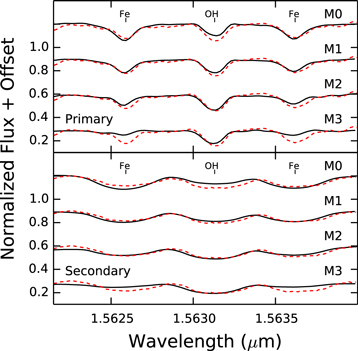
Figure 5. Spectra of the 1.563 μm region in order 49 showing the primary component (top panel, solid black lines) and secondary component (bottom panel, solid black lines) compared to M0, M1, M2, and M3 spectral standard stars (dashed red lines). The standards have been veiled and rotationally broadened to match the observed spectra. The veiling and rotational broadening applied to the templates are 0.6 and 13 km s−1 for the primary, and 0.0 and 41 km s−1 for the secondary, respectively. The relative depths of the OH (1.5627 μm) and Fe lines (1.5623 and 1.5631 μm), after veiling and rotational broadening, were used to estimate the spectral types of the components.
Download figure:
Standard image High-resolution image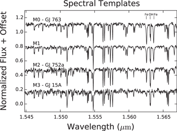
Figure 6. Full order 49 spectral sequence of standards used in this work. The relative depths of the OH (1.5627 μm) to Fe lines (1.5623 and 1.5631 μm) change starkly as a function of effective temperature and were used to determine the spectral types of the DF Tau components. Spectra and information about the templates can be found at: (http://www2.lowell.edu/users/lprato/hband/homepage.html). The template labeled M1 is an average of the M0 and M2 templates.
Download figure:
Standard image High-resolution imageTable 8. Spectroscopic Standard Stars
| Object | Spectral Type | BJD | vrad |
|---|---|---|---|
| GJ 763 | M0 | 2451715.10901 | −63.16 |
| GJ 752A | M2 | 2451706.03321 | 35.73 |
| GJ 15A | M3a | 2451707.14155 | 11.82 |
Note.
aFrom Prato (2007).Download table as: ASCIITypeset image
3.3. Veiling and v sin i
Veiling is a continuum emission component that has the effect of making the spectral absorption lines shallower. It is often assumed to be a linear function of wavelength, and over short wavelength intervals (narrow atomic and molecular lines) can be approximated by a constant (Hartigan et al. 1989). We assume a constant veiling of r that contributes to a spectrum, s, that has been continuum normalized to unity (Basri & Batalha 1990), as

The inclination modulated rotational velocity,  , can be determined by the Doppler broadening of the spectral absorption lines. We added veiling and rotational broadening to the blended OH doublet at 1.5627 μm in template spectra with no veiling and known (low) rotational velocity to create models with which to simultaneously estimate DF Tau's veiling and
  . The OH feature is ideal for this purpose because of its relative insensitivity to magnetic fields (O'Neal et al. 2001). The veiling component was added to the spectrum using Equation (2) and the rotational broadening was applied using the PyAstronomy7
function RotBroad, assuming a limb-darkening parameter of
. The OH feature is ideal for this purpose because of its relative insensitivity to magnetic fields (O'Neal et al. 2001). The veiling component was added to the spectrum using Equation (2) and the rotational broadening was applied using the PyAstronomy7
function RotBroad, assuming a limb-darkening parameter of  (Claret et al. 1995). To determine the veiling and
  of the DF Tau components, we applied a range of veiling values from 0 to 10 in increments of 0.1 and a range of broadening kernels ranging in magnitude from 0 to 100 in increments of 1 km s−1 to the spectra of our standard stars shown in Figure 6 and listed in Table 8 (Prato et al. 2002; Bender et al. 2005; Prato 2007).
For each set of veiling and  values we determined the minimum reduced
  . Veiling and
  were also determined using the Fe i lines at 1.5623 and 1.5631
  the results were consistent with those determined using the OH doublet. Table 9 lists the veiling and
  estimates determined for the DF Tau components using the M2 template, GJ 752A, which provided the best match. If we take the average over the three epochs and consider the maximum range in values determined for each epoch to be indicative of the uncertainty, then the primary has a veiling of 0.6 ± 0.1 and a
  of 13 km
  km s−1. Similarly, the secondary has a veiling of 0.0 ± 0.1 and a
  of 41 km
  km s−1. To confirm our results for these values of veiling and
  we repeated the analysis for order 47, which is also relatively free of telluric lines, and obtained similar results. For the primary component we measure a veiling of 0.6 ± 0.1 and a
  of 10 km
  km s−1. For the secondary we measure a veiling of 0.0 ± 0.1 and a
  of 43 km
  km s−1. The results are shown in Figure 7. In our subsequent analysis we used the values determined from order 49.
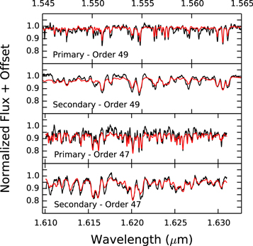
Figure 7. The top two panels show the full order 49 NIRSPEC spectra for the primary component (above) and secondary component (below) compared to the veiled and rotated M2 standard star, GJ 752A. The lower panels show the results of the same analysis for order 47.
Download figure:
Standard image High-resolution imageTable 9. v sin i and Veiling Estimates
| Epoch | Component | Template | Line | Veiling |

|
|---|---|---|---|---|---|
| 2009 | A | M2 | OH | 0.7 | 9.0 |
| 2010 | A | M2 | OH | 0.6 | 13.0 |
| 2013 | A | M2 | OH | 0.6 | 14.0 |
| 2009 | A | M2 | Fe1 | 0.3 | 11.0 |
| 2010 | A | M2 | Fe1 | 0.2 | 13.0 |
| 2013 | A | M2 | Fe1 | 0.3 | 14.0 |
| 2009 | A | M2 | Fe2 | 0.3 | 11.0 |
| 2010 | A | M2 | Fe2 | 0.1 | 13.0 |
| 2013 | A | M2 | Fe2 | 0.3 | 16.0 |
| 2009 | B | M2 | OH | 0.0 | 41.0 |
| 2010 | B | M2 | OH | 0.0 | 40.0 |
| 2013 | B | M2 | OH | 0.0 | 41.0 |
| 2009 | B | M2 | Fe1 | 0.1 | 33.0 |
| 2010 | B | M2 | Fe1 | 0.0 | 34.0 |
| 2013 | B | M2 | Fe1 | 0.0 | 35.0 |
| 2009 | B | M2 | Fe2 | 0.0 | 34.0 |
| 2010 | B | M2 | Fe2 | 0.0 | 34.0 |
| 2013 | B | M2 | Fe2 | 0.0 | 36.0 |
Download table as: ASCIITypeset image
Our  estimates are similar to those of Nguyen et al. (2012), 46.6 km
  km s−1 for the primary and 9.8 km
  km s−1 for the secondary. These component values are the reverse of ours, with the secondary identified as the slow rotator and the primary identified as the rapid rotator. This is likely because, although Nguyen et al. (2012) could spectroscopically resolve the system as a double-lined binary, they were unable to spatially resolve the two components. It is likely that the confusion arose given the similarity in spectra types.
3.4. Radial Velocity Determination
Radial velocities for the individual component-resolved spectra were determined via one-dimensional cross-correlation against the spectral template, GL 752A, rotationally broadened and veiled to match the individual component spectra (Section 3.3). RVs for the resolved spectra are listed in Table 10. The resolved component RVs span a time period equal to roughly 10% of the orbital period of the system. Thus, we can compare these measured RVs with the predicted RVs calculated from the parameters in Section 3.1, assuming the components are of equal mass (Section 3.2). The spectroscopic orbit can resolve the 180° ambiguity between the argument of periastron (ω) and the position angle of the line of nodes (Ω) in the visual orbit. We find that the differences in the component RVs are consistent with  . The resolved component RVs are plotted as a function of orbital phase in Figure 8.
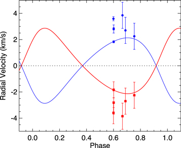
Figure 8. Relative RVs of the components of DF Tau as a function of orbital phase, assuming equal component masses. The blue and red lines show the predicted RVs for the primary and secondary, respectively, from the orbital solution described in Section 3.1. The filled blue squares and red dots are the measured RVs for the primary and secondary, respectively, measured from the resolved spectra with an angle between the node and periastron  of 129
 2. The three data points at higher phases show our NIRSPEC data. The other points represent the RVs measured by Nguyen et al. (2012), in good agreement with our results, although it appears that their uncertainties are underestimated. Our RVs were measured by cross-correlation of the angularly resolved NIRSPEC spectra with the standard star GL 752A convolved with a rotation kernel to mimic a
  of 13 km s−1 for cross-correlation with the primary and 41 km s−1 for cross-correlation with the secondary. We calculated the difference in the primary and secondary RVs for each of the epochs and divided it by two, assuming equal component masses.
Download figure:
Standard image High-resolution imageTable 10. Component-resolved Radial Velocities
| Component | Date | Template | RV | Error |
|---|---|---|---|---|
| (JD) | (km s−1) | (km s−1) | ||
| 2009 A | 2455171.914880 | GJ 752A | 17.2 | 1.0 |
| 2009 B | 2455171.914880 | GJ 752A | 9.5 | 1.0 |
| 2010 A | 2455542.85277 | GJ 752A | 14.8 | 1.0 |
| 2010 B | 2455542.85277 | GJ 752A | 9.4 | 1.0 |
| 2013 A | 2456648.761910 | GJ 752A | 14.9 | 1.0 |
| 2013 B | 2456648.761910 | GJ 752A | 10.4 | 1.0 |
Download table as: ASCIITypeset image
The unresolved spectra span only 2% of the orbital period. Therefore, we expect to see little change in their measured radial velocities. To test this we cross-correlated the unresolved spectra with each other using the best signal-to-noise spectrum (UT 2001 December 31) as the template (Table 11). The relative RVs measured for these spectra are less than our uncertainty of 1 km s−1.
Table 11. Unresolved Radial Velocities
| Spectrum | Date | Template | RV | Error |
|---|---|---|---|---|
| (JD) | (km s−1) | (km s−1) | ||
| 2002-2-5 | 2452310.74795 | 2001-12-31 | 0.9 | 1.0 |
| 2002-7-18 | 2452474.11428 | 2001-12-31 | −0.3 | 1.0 |
| 2002-10-30 | 2452578.11096 | 2001-12-31 | 0.3. | 1.0 |
| 2002-12-14 | 2452622.88648 | 2001-12-31 | −0.3 | 1.0 |
Download table as: ASCIITypeset image
3.5. Spectral Energy Distributions
Figure 9 shows the observed spectral energy distributions (SEDs) of the individual components of DF Tau derived from the photometry described in Section 2.5. Also plotted are the observed, unresolved Spitzer IRAC and WISE photometry results. The photometry was dereddened using  , based on the range of values for AV in the literature that range from ∼0.15 mag (White & Ghez 2001) to ∼0.75 mag (Hartigan & Kenyon 2003). Both components have a similar flux in the I-band; however, the primary component has strong excess flux compared with the secondary in both the ultraviolet (UV) and near-infrared (NIR) regions of the SED. The IR excess of the system continues into the mid-infrared and also into the submillimeter (Andrews & Williams 2005; Harris et al. 2012), although the latter is not shown in Figure 9.
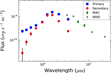
Figure 9. Spectral energy distributions for both components of DF Tau. The blue squares and red circles are the dereddened visible and NIR photometry of the primary and secondary, respectively. The green diamonds are unresolved photometry at the [5.8] and [8.0] Spitzer bands and the green stars are unresolved WISE photometry. The submillimeter measurements of Andrews & Williams (2005) and Harris et al. (2012) are not plotted. Most of the uncertainties are smaller than the plotted points.
Download figure:
Standard image High-resolution imageIn Section 3.2 we determined the spectral types of the DF Tau components. We can compare the colors of the components against the expected colors of a young star with the same spectral type. Table 12 gives the dereddened U − B, B − V, J − H, J − K, and K − L colors for both components, as well as the intrinsic colors of a representative young M2 star from the tabulation of Pecaut & Mamajek (2013). The colors of the secondary component are mostly consistent with the colors expected from photospheric emission, except for a weak U − B and K − L excess. The strong NIR excess of the primary indicates that it has a dusty, optically thick inner disk, while its UV excess likely indicates active accretion. The NIR colors of the secondary and weak UV excess are consistent with the absence of an inner disk.
Table 12. Dereddened Colors of DF Tau and a Young M2 Photosphere
| Component |

|

|

|

|

|
|---|---|---|---|---|---|
| A | −0.53 ± 0.08 | 0.59 ± 0.064 | 0.96 ± 0.07 | 1.61 ± 0.05 | 0.88 ± 0.17 |
| B | 0.49 ± 0.31 | 1.2 ± 0.16 | 0.74 ± 0.09 | 0.97 ± 0.09 | 0.37 ± 0.17 |
| M2 | 1.17a | 1.46b | 0.67b | 0.9b | 0.14c |
Notes.
aColor from Kenyon & Hartmann (1995). bColor from Pecaut & Mamajek (2013). c color from Pecaut & Mamajek (2013).
Download table as: ASCIITypeset image
3.6. Circumstellar Disk Properties
Both White & Ghez (2001) and Hartigan & Kenyon (2003) found strong evidence for an accreting circumstellar disk around the primary. White & Ghez (2001) concluded that there is a disk based on a measured U-band photometric excess. Hartigan & Kenyon (2003) based their determination on the presence of Hα emission, veiling, and [O i] emission. We found strong evidence for a circumstellar disk around the primary star. The NIR colors listed in Table 12, including a dereddened K − L color of 0.88 ± 0.17 mag, are indicative of an optically thick inner circumstellar disk around the primary star. The veiling and U − B color measured for the primary star are also consistent with an accreting circumstellar disk.
White & Ghez (2001) and Hartigan & Kenyon (2003) also argued for the presence of a circumstellar disk around the secondary star. White & Ghez (2001) based their conclusion on a weak U-band excess and Hartigan & Kenyon (2003) based their conclusion on the presence of Hα emission, veiling, and [O i] emission. We found little evidence for a disk around the secondary star and no indication of accretion, implying at best the presence of sparse circumstellar material. The NIR colors of the secondary are consistent with photospheric emission from the star, with the exception of the dereddened K − L color, 0.37 ± 0.17, which is marginally indicative of emission from warm dust. Additionally, we measured no veiling in the spectrum of the secondary star. The K-band flux ratio of the primary to secondary stars is ∼2, suggesting the presence of an optically thick inner circumstellar disk around the primary, increasing its brightness as the result of accretion and thermal emission from warm dust. It is possible that the disk signatures seen in Hartigan & Kenyon (2003) for DF Tau B could be the result of contamination from the strong emission from DF Tau A: the system separation of less than  is roughly equal to the STIS spatial resolution in the visible, thus their resolution was marginal at best.
Assuming that all observations of DF Tau that trace disk processes are probing material around the primary, we can use unresolved as well as resolved data to characterize the size of DF Tau A's disk. HST STIS spectroscopy of the DF Tau system (Herczeg et al. 2006) showed H2 emission consistent with an origin on the surface of a warm disk. Observations of CO molecular line emission from the inner disk gas were obtained by Salyk et al. (2011) with NIRSPEC on Keck II, and observations of H2 lines in the far-UV were obtained by France et al. (2012) with COS on HST. These molecular emission line observations led both groups to estimates of the inner disk radius of 0.1 au and 0.06 au, respectively. Dynamical constraints can be placed on the outer edge of the disk. Models from Artymowicz & Lubow (1994) show that, as the result of truncation by the companion, for an equal-mass, co-planar, binary system, a circumstellar disk can have an outer radius of roughly  , where a is the semimajor axis. The DF Tau system has a separation of 14 au (Section 3.1, Table 7), thus the outer disk radius of the primary must be <5 au.
3.7. Photometric Variability
3.7.1. Observations
Photometric variations of stars can provide information on both the rotation periods, from measurements of periodic variability, and accretion rates, from measurements of aperiodic outbursts. There is a rich history of photometric observations of DF Tau, demonstrating variability on timescales from hours to years and in brightness of up to 1.5 mag in the V-band and up to 3 mag in the U-band (Zaitseva & Liutyi 1976; Shevchenko & Shutemova 1981; Rydgren et al. 1984; Walker 1987; Bouvier & Bertout 1989; Richter et al. 1992; Bouvier et al. 1993, 1995; Herbst et al. 1994; Johns-Krull & Basri 1997; Lamzin et al. 2001; Grankin et al. 2007; Percy et al. 2010; Xiao et al. 2012). We examined the photometry of the DF Tau components, as well as that of the unresolved system for which we interpret the periodic results in terms of the rotation of the primary star given the dominant flux of the primary at most wavelengths.
Figure 10 shows the angularly resolved V-band photometry acquired by the Hubble Space Telescope FGS over a decade (Schaefer et al. 2003, 2006). The largest photometric variability attributable to the presence of dark spots on a rotating star is on the order of a magnitude or less (Nolthenius 1991; Strassmeier & Olah 1992). The DF Tau primary shows highly variable behavior in excess of 1.5 mag. It is thus likely that a number of phenomena, in addition to cold spots, contribute to these changes, including active accretion flows, hot spots, occultation by circumstellar material, and other processes indicative of the presence of an optically thick circumstellar disk. Variability in the DF Tau secondary is low at the 0.2 mag level. Given the extremely sparse sampling of these FGS data over the 10 years of observation, it was possible to extract only approximate rotation periods for each component individually.
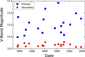
Figure 10. Reconstruction of the HST Fine Guidance Sensor V-band photometry of DF Tau from Schaefer et al. (2003, 2006). The primary photometry is in blue and the secondary photometry is in red. In addition to being fainter, the secondary has much less peak-to-peak photometric variability (0.2 mag) than the primary (1.4 mag). Typical uncertainties are around 0.35 mag.
Download figure:
Standard image High-resolution imageFor our analysis of the unresolved system, we assumed that the variability is the result of flux changes in the primary component because of the long-term lack of variability seen for the secondary component in the HST FGS data (Figure 10). Although it is not unprecedented that the variability of a young star is itself variable, the FGS data for the secondary spans ∼10 years of quiescence and only low-level variability. As discussed in Section 3.5, and discussed further in subsequent sections, every indication of the SED and other properties of DF Tau B point toward a weak-lined T Tauri star devoid of circumstellar material. Herbst & Shevchenko (1999) demonstrated in their Figure 2 that the typical V-band variability of weak-lined, diskless T Tauris, <0.5 mag, is much lower than that for classical, disk-bearing T Tauris, up to 3 mag or more. With the exception of the I-band, the DF Tau primary dominates the unresolved system flux at all wavelengths, and it is highly likely that it also dominates the variability. It is a reliable assumption, therefore, that most periodic variability, as well as the majority of the aperiodic variability, arises in the primary star.
Several groups have used light curves to study DF Tau's rotation (Bouvier & Bertout 1989; Bouvier et al. 1995; Percy et al. 2010). A range of rotation periods has been measured, including 8.5 days (Bouvier & Bertout 1989), 8.9 days (Bouvier et al. 1995), 7.9 days (Richter et al. 1992), and 7.0 days (Johns-Krull & Basri 1997). Not all attempts to determine a period for DF Tau have been successful, however. For example, using archival CCD photometry, (Percy et al. 2010) and TrES photometry (Xiao et al. 2012), no rotation period was recovered. A periodogram analysis of 175 V-band observations of DF Tau cataloged in Herbst et al. (1994) did not recover a period either.
A Lomb–Scargle periodogram analysis of the primary star FGS photometry (Figure 10) yielded a period of 7.5 days and a false alarm probability (FAP) of 19%. Although this is not a robust result, it is consistent with the previous estimates in the literature given above. To determine a more reliable outcome, we applied a Lomb–Scargle periodogram analysis to our B-, V-, and I-band photometric data sets from the Lowell Observatory 0.8 m telescope spanning 131 angularly unresolved observations taken over 119 days. We used the astroML8 (Ivezić et al. 2014) implementation of the generalized Lomb–Scargle routine (Zechmeister & Kürster 2009) to search 10,000 periods with a range of 1.5–20 days. Figure 11 shows the power spectrum for the V-band and the window function over the range of periods explored. There is a peak at 10.5 days that is much stronger than that of any other peak. The associated FAP is <0.0001%. This analysis was performed for the B and I-band data as well, with a similar result. The only apparent differences were a larger amplitude in the B-band and a smaller amplitude in the I-band compared to the V-band. Given the decreasing photosphere-spot contrast at longer wavelengths (e.g., Prato 2007), these differences in amplitude are unsurprising.

Figure 11. Lomb–Scargle periodogram analysis of the V-band 0.8 m photometry. The strongest peak occurs at a period of 10.5 days. Analyses of the B- and I-band data give the same result. The red dashed line is the window function.
Download figure:
Standard image High-resolution imageA periodogram analysis of the angularly resolved FGS data for the secondary star resulted in a rotation period of 3.0 days with an unreliably high FAP of 35%. We also used our unresolved data and searched for periodicity associated with the secondary star by subtracting a sinusoid with a period determined from the peak of the periodogram (Figure 11) and amplitude and phase determined from fitting to the light curve (Figure 12). In Figure 12, most of the deviations from the fit that occur are increases in brightness, consistent with accretion events. Figure 13 shows the periodogram of the residual light curve. Also plotted in Figure 13 are the locations of the two peaks in the original periodogram, Figure 11. In the periodogram of the residual light curve these correspond to local minima, implying that the secondary peak in Figure 11 at ∼9.3 days is not a true recovered rotation period.
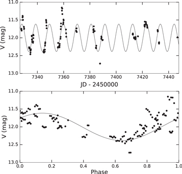
Figure 12. Observed light curve (top) and phased light curve (bottom) from the 0.8 m V-band photometry. The best-fit sinusoid, assuming a Prot of 10.5 days, is overplotted in both panels. Uncertainties are smaller than the plotted points.
Download figure:
Standard image High-resolution image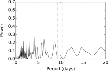
Figure 13. Lomb–Scargle periodogram analysis of our V-band photometry after subtraction of the best-fit sinusoid, assuming a Prot of 10.5 days, shown in Figure 12. The two dashed lines show the location of the two strongest peaks in Figure 11.
Download figure:
Standard image High-resolution image3.7.2. Modeling
In spite of our conclusions above about the 9.3-day period not corresponding to the rotation of the secondary, we nevertheless considered that case and have explored this possibility further by modeling the unresolved photometry. Irregular sampling of observations can also produce large peaks as the result of aliasing, which can be tested. We created a model binary and simulated the unresolved photometric variability of the system following the prescription of Aigrain et al. (2012) for the time-series photometric signature observed in the presence of starspots on a rotating star. We modified the procedure to generate the unresolved photometric signal of two rotating stars in a binary system, rendering it applicable to modeling the observed signature of DF Tau.
In Figure 14 we show the periodograms from all three of our observed bandpasses compared with the averaged periodogram output of 10,000 iterations of simulated light curves of an unresolved binary system given three sampling frequencies: (1) identical to the cadence of our observations, (2) evenly spaced sampling on a nightly, 12 hr basis, and (3) evenly spaced sampling without nightly restrictions, i.e., continuous over 24 hours. The primary component's rotation period was set to 10.5 days as determined in Section 3.7.1; a rotation period of 9.3 days was imposed on the secondary. The simulations were based on the flux ratios derived from component magnitudes (White & Ghez 2001) for each corresponding bandpass and a level of variability corresponding to that observed in the FGS data. As discussed above, the diskless nature of the secondary star indicates that its variability is likely on the order of or less than V = 0.5 mag (Herbst & Shevchenko 1999). Stellar limb-darkening was not taken into account because even though the stellar unspotted photospheric brightness decreases toward the limb, so does the brightness of the spots, minimizing the photometric signature of the spot.
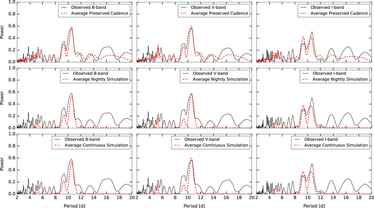
Figure 14. Left, middle, right Columns: B-, V-, and I-band power spectra. Top row: power spectra of B-, V-, and I-band time-series photometry acquired with the Lowell 0.8 m Telescope (solid black) compared to the averaged power spectrum of 10,000 light curve simulations with the same sampling cadence as the 0.8 m observations (red dashed). Middle row: same as top row, except simulations were performed with an even sampling cadence on a "nightly" basis. Bottom row: same as top row, except simulations were performed with even sampling, ignoring nightly observing restrictions. All simulations performed assume that the primary rotation period is 10.5 days and that the secondary rotation period is set to 9.3 days.
Download figure:
Standard image High-resolution imageIf the 9.3-day signal in DF Tau's observed periodogram is indeed evidence of the secondary component's rotation period, then the same periodogram analysis of the simulated light curves described above should produce a signal corresponding to 9.3 days with a strength that is comparable to that seen in the observed periodogram, regardless of the sampling frequency. This is not seen for any bandpasses in this study. In both the B and V bands, the periodograms' 9.3-day signal strength imposed on the secondary rotation period decreases for light curves that were modeled with both evenly spaced nightly and continuous sampling frequencies. This indicates that the strength of the secondary signal in the periodogram is, in part, an effect of the spacing between observations.
Although still apparent, this effect contributes much less to the strength of the 9.3-day signal in the I-band simulations; in fact, the simulated signal strength is similar to the observed strength. However, the overall shape of the model periodogram does not resemble the observational results because the secondary component flux is comparable to the primary's in the I-band, so both respective periodic brightness modulations contribute to the light curve approximately equally. This behavior is reflected in the results from all I-band simulations, which show equally strong signals at both 9.3 days and 10.5 days. This expectation is not met by the 0.8 m observations and provides supporting evidence that the 9.3-day periodic signal is not the rotation period of the secondary component. We also created models for the case in which both binary components varied by the range of magnitudes seen for the primary star in the FGS data (Figure 10). The results of these models failed to accurately fit the primary observed peak at 10.5 days for all sampling frequencies.
We performed a final check of the 9.3-day peak by simulating a light curve with only one period. We model the light curve using a sinusoid with a 10.5-day period and coefficients determined from the observed light curve. The simulated light curve and phased light curve, using the same cadence as the observations, are shown in Figures 15 and 16. Even though the only periodicity in the simulated light curve is 10.5 days, there is a secondary peak in the periodogram at 9.3 days. We conclude that the 9.3-day peak does not represent the secondary star's rotation period.
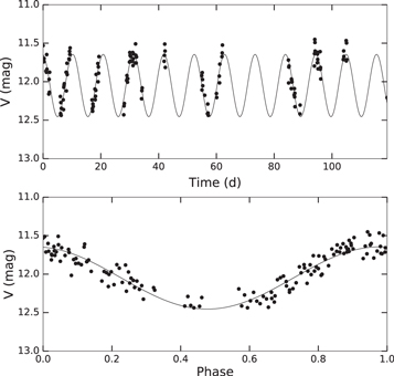
Figure 15. Simulated light curve (top) and phased light curve (bottom) for a single spotted star determined from the sinusoidal fit to the observed light curve in Figure 12.
Download figure:
Standard image High-resolution image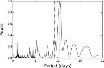
Figure 16. Periodogram of the simulated light curve. Even though the simulated light curve only included a single 10.5-day periodicity, a peak at 9.3 days is still apparent. The two dashed lines show the location of the two strongest peaks in Figure 11.
Download figure:
Standard image High-resolution image
Although evidence suggests the 9.3-day periodic signal is not the rotation period of the secondary, the FAP of this peak is 0.00 (within precision) for the B-, V-, and I-band observations, suggesting that the signal may be astrophysical in nature. Various processes common to classical T Tauri star systems may produce a periodic flux, such as accretion hot spots or clumpy inhomogeneities in the inner wall of a circumstellar disk. Further investigation of these phenomena is beyond the scope of this work; however, we will explore accretion-related origins for this signal in a future publication (L. I. Biddle et al. 2017, in preparation).
3.7.3. Rotation Periods and Inclinations
The significant discrepancy in our  measurements for each of the approximately equal-mass DF Tau components, similar to the results of Nguyen et al. (2012), indicates either markedly different stellar inclinations or different rotation velocities, or some combination of both. Solving for the sin of the inclination in terms of the rotation period, Prot, in days, the
  , in km s−1, and the stellar radius R in terms of
  we find:
For the measured primary star rotation period, 10.5 days, and  , 13 km s−1, this yields

The radius of the primary star must therefore be 2.68 R⊙ for an inclination of 90°, i.e. perpendicular to our line of sight, or >2.68 R⊙ for a lower inclination. Model radii for young stars of similar mass (0.55M⊙; Section 3.2), effective temperature, Teff (3490 K for an M2 star; Pecault & Mamajek 2013), and age (1–2 Myr; Schaefer et al. 2014) are typically less than 2.68 R⊙ (e.g., McClure et al. 2013; Baraffe et al. 2015). Converting from the apparent V magnitude (Table 6) of the diskless secondary star to bolometric luminosity and adopting Teff = 3490 K, we use L = 4πR2σTeff4 to estimate component radii of ∼2.1 R⊙ for the M2 stars in the DF Tau system. Given the ±4 km s−1 1σ uncertainty in our v sin i measurement for the primary star, the limiting radius for sin i ≤ 1 could be as small as 1.85 R⊙, consistent with our radii estimate and current model values. Nevertheless, it is most likely that the DF Tau A rotation axis inclination is close to 90°.
If we take the ratio of Equation (3) for the components DF Tau A and B and assume equal radii given the equivalent spectral types and masses we find

For  , the other values for DF Tau A given above, and a
  of 41 km s−1, this reduces to

This relation implies that the rotation period for DF Tau B must be on the order of 3.33 days for an inclination of DF Tau A of 90°; any longer rotation period is unphysical for the case of  . This result is consistent with the results of the periodogram analysis, 3.0 days, for the angularly resolved FGS data. Alternatively, if
  is less than one,
  may be longer than 3.33 days. If we assume that the 9.3-day signal in the power spectrum of the unresolved DF Tau system (Figure 14) does represent the secondary star's rotation period, we can invert the process followed here in Equations (3) through (5) to determine the required primary star radius to be consistent with a value of
  of 9.3 days. This yields the unphysical result of
  , adding weight to the modeling results discussed in Section 3.7.2 that point to an origin for the 9.3-day power spectrum signal that is unrelated to the rotation of the secondary star.
Because of the degeneracy in the interplay between the stellar radii and the unknown secondary star rotation period, it is not possible to definitively measure the stellar inclinations. However, given that the lower limit for the radii is larger than any predicted by recent models, we surmise that the value for the primary star's radius of  is likely correct and therefore that the primary star's inclination is likely to be ∼90°. Correspondingly, for the secondary star, Prot must be 3.33 days or shorter; for
  days the inclination of the secondary is also 90°. We are optimistic that the results of the recently concluded Kepler K2 campaign in the Taurus star-forming region, when public, should unambiguously reveal the DF Tau A and B rotation periods; DF Tau was on silicon for that campaign.
4. Discussion
DF Tau is an unusually well characterized young binary in that we have determined the parameters of the ∼44 year orbit as well as angularly resolved photometry and high-resolution spectroscopy of each individual component. Copious unresolved data were also collected by our team and are available in the literature. Additional high-value data, such as a likely measurement of both stellar rotation periods from K2 (e.g., Rebull et al. 2017) and ALMA images of the DF Tau A circumstellar disk, are being currently processed or will soon be proposed.
The individual component spectroscopy enabled by high-resolution IR spectroscopy behind the Keck II AO system showed, remarkably, that both components of DF Tau are of equal spectral type and thus of similar, if not equal, effective temperature, radius, and mass. However, this spectroscopy also revealed marked differences in the projected component rotation velocities. While the primary star  is only 13 km s−1, the secondary
  is 41 km s−1. This could be the result of either discrepant inclinations or rotation velocities. The circumstellar properties of these twin stars offer a clue: while DF Tau A displays strong evidence for an actively accreting, dusty disk given the significant veiling, UV, and IR excesses, DF Tau B displays none of these characteristics. It is thus tempting to attribute the lack of rotational modulation from disk-locking to a rapid rotational velocity for DF Tau B.
This scenario is supported by our investigation of the component rotation periods by means of both angularly resolved and unresolved photometry. Although the FGS data were sparsely sampled and associated with a high FAP, the 3-day FGS period is consistent with the limiting case for  days for DF Tau B (Section 3.7.3). The ∼7.5-day FGS period for DF Tau A is also associated with a significant FAP but is coincident with some estimates in the literature and not highly discrepant with our results, based on the periodogram analysis of our unresolved data, 10.5 days with a FAP of <0.0001%. We used both modeling and the limiting cases of viable parameters (Sections 3.7.2 and 3.7.3) to demonstrate that the 9.3-day period seen in the periodogram analysis of the unresolved photometry is unrelated to the rotation of DF Tau B. The slow rotation of DF Tau A is therefore consistent with disk-locking and the rapid rotation of DF Tau B is consistent with the absence of an inertial circumstellar reservoir.
Assuming that the DF Tau binary components are at least approximately coeval, which is highly probable given their 14 au semimajor axis, the puzzle becomes why, in a system of two at least approximately equal-mass stars, should one have a disk which evolves more rapidly than the other. A variety of mechanisms can destroy circumstellar disks around young stars, including close stellar companions, other dynamical interactions, photoevaporation from the host star, ionizing flux in a hostile environment, and planet formation. Apparent inequality in the disk properties of a binary pair may also be the result of specific initial conditions or divergent accretion histories. We discuss disk dissipation mechanisms and their relevance to the DF Tau system. Alexander et al. (2014) provide a general review of these processes.
Observations of binary systems in Taurus (Harris et al. 2012) demonstrated a clear decrease in submillimeter emission, used as a proxy for disk mass, as a function of decreasing binary separation. Kraus et al. (2016) found a similar result on the basis of optical can IR disk diagnostics. This is consistent with theoretical calculations that show that, for close binary systems, disk radii can be at most ∼1/3 of the orbital separation (Artymowicz & Lubow 1994). A separation of 14 au for the components in DF Tau imposes an upper limit on the outer disk radius, around either star, of 5 au. This, however, does not account for the absence of an inner circumstellar disk around DF Tau B. If this star was itself composed of a tight binary, its inner disk could have been affected. This scenario, however, is unlikely. Both the photometric stability, the stability of the visual orbit, and the correspondence between measured and predicted radial velocities (Figure 8) and the astrometry (Figure 4) argue against the binary nature of the secondary star. We also cross-correlated the three epochs of spectroscopy for DF Tau A with each other and the three for DF Tau B with each other; no evidence for either component being a spectroscopic binary was detected.
The host star can destroy a disk via photoevaporation and winds. High-energy X-ray and UV photons incident on the surface of the disk can provide enough energy to overcome the gravitational potential and launch a pressure-driven wind (Alexander et al. 2014). The mass-loss profile (mass-loss rate versus radius) of a disk depends on the wavelength of the incident radiation and peaks at ∼1 au for EUV models, ∼3 au for X-ray models, and ∼3–10 au for FUV models. The peak mass-loss rates vary by a large amount, with FUV photoevaporation ( ) dominating over X-ray photoevaporation (
 ) and EUV photoevaporation (
 ). Photoevaporation only dominates after the disk surface density drops below a critical value of ∼1 g cm−2. Once this occurs, disks can dissipate rapidly (Alexander et al. 2014). Furthermore, disk destruction resulting from photoevaporation driven by the host star is more effective around intermediate and higher-mass stars than around low-mass stars. Because both stars in the DF Tau system are of approximately the same low mass, it is unlikely that one disk has been destroyed by photoevaporation while the other has not.
Alexander (2012) explored models of photoevaporation in binary systems and found that binary separation has a notable impact on disk lifetime. Very close binaries (<1 au) can suppress accretion, keeping the disk surface density above the critical surface density, and thus may have longer disk lifetimes than single stars. As binary separation increases toward 10–12 au, the disk lifetime decreases. This result, however, does not explain why disk destruction would be accelerated around only one star in a binary system.
The local environment that a star forms in can have a profound affect on the lifetime of its circumstellar disk. Disks can be photoevaporated and destroyed because of the radiation fields of high mass neighbors (Adams et al. 2004). This process has been observed in the Orion nebular cluster near the massive O stars of the Trapezium (Bally et al. 1998). However, such processes only occur in proximity to massive O stars, and even in that case it is not necessarily clear what degree of disk destruction can be attributed to this mechanism (Allen et al. 2012). In dense cluster centers, close encounters with other cluster members can truncate disks (Vincke et al. 2015). The stellar density of the Taurus star-forming region, however, is relatively low, with few massive stars likely to interact closely enough with neighbors to truncate their disks. Furthermore, given the DF Tau binary semimajor axis of only 14 au, any external influence should affect both components. Thus, it is unlikely that the disk around DF Tau B was destroyed as the result of external influences.
Planet formation is another process that can disrupt protoplanetary disks. Planets can carve out gaps in disks and inhibit the flow of material within the orbital radius of the planet. This allows the disk inside of the planet to accrete onto the star. The remaining material outside the planet's orbit is then photoevaporated away on short timescales (Alexander et al. 2014). Over the past decade, planet searches have yielded thousands of planets and planetary candidates (e.g., Coughlin et al. 2016), and planetary systems are now considered common. Binary and higher-order multiple systems have been found to host numerous planets. This raises the question of whether planet formation alone could be responsible for the destruction of the disk around DF Tau B. If planet formation were to happen early in the evolution of the star+disk system, while a circumstellar envelope was still present, the planet could quickly accrete to brown dwarf/low-mass star size (Kratter et al. 2010; Jang-Condell 2015). The only way to avoid this scenario would be to have a planet form exactly at the end of the epoch of envelope dispersal, late enough not to accrete into a brown dwarf but early enough to destroy an accretion disk, which is unlikely.
We also consider differences in the initial conditions of the disks, or differences in their evolutionary histories. Young stars can accrete around 10% of their final mass during the CTTS stage (Hartmann & Kenyon 1990). Although accretion rates generally decrease as young stars age (Hartmann et al. 1998), these rates are time variable and episodic, capable of reaching high rates ( yr−1) for short periods of time (Hartmann et al. 1993). This implies that disk evolution can proceed rapidly during short time spans, and consequently that the accretion history of a disk can affect its lifetime. Magnetospheric accretion models allow for steady flows via magnetic "funnels," as well as Rayleigh–Taylor unstable accretion via equatorial flows, and can cycle between regimes (Romanova et al. 2008). The large possible range of accretion histories can allow for a large range in potential disk mass outcomes.
DF Tau is not unique as a binary with only a single circumstellar disk (e.g., Prato & Monin 2001; White & Ghez 2001). Prato et al. (2001) and Kellogg et al. (2017) speculate that dynamical interactions, even between wide components with orbits of hundreds of years, have the capacity at the several Myr ages of T Tauri stars to evolve with thousands of crossing times, particularly to the detriment of a disk with an orientation susceptible to instability with orbital motion, i.e., perpendicular to the orbital plane. We plan to propose ALMA observations at the highest possible angular resolution to determine the orientation of the DF Tau A disk with respect to the relatively well-characterized binary orbit. This geometric information may at least provide into the longevity of the disk that is still present.
5. Summary and Conclusions
We present NIR spectroscopy and imaging of the young binary system DF Tau and determine  , veiling, spectral type, RV, mass, and circumstellar disk evolutionary state for the individual stars in the system. We used estimates of the rotation period of the primary star to place limits on the rotation period of the secondary, demonstrating that the Prot of the secondary is likely ∼3 times faster than that of the primary. DF Tau appears to be a system in which one component is disk-locked and the other has spun up after the onset of disk dissipation. Out of the possible scenarios leading to the difference in disk presence around the components of DF Tau, initial differences in disk properties or accretion histories are the most plausible. It is possible that not all young stars emerge from the protostellar stage with disks at all, or with comparable disks, both in terms of mass and geometry, a conclusion with implications for the study of disks around young single stars as well as young binaries.
The authors would like to thank Christopher Johns-Krull, Otto Franz, Joe Llama, Audrey Thirouin, and Alison Crocker for insightful discussion and comments. This research was supported in part by NSF grant AST-1313399 and the associated REU supplement, AST-1641417 (to LP). G.H.S. acknowledges support from NSF Grant AST-1411654; L.P. and G.H.S. were also supported by NASA Keck PI Data Awards, administered by the NASA Exoplanet Science Institute. The work of R.M. was supported in part by the Northern Arizona University Research Experience for Undergraduates program through NSF grant AST-1461200. We thank the referee for comments that improved the presentation of this manuscript. This research has made use of data products from the SIMBAD reference database, the NASA Astrophysics Data System, the Wide-field Infrared Survey Explorer, a joint project of the University of California, Los Angeles, and the Jet Propulsion Laboratory/California Institute of Technology, funded by the National Aeronautics and Space Administration, and the Two Micron All Sky Survey, a joint project of the University of Massachusetts and the Infrared Processing and Analysis Center/California Institute of Technology, funded by the National Aeronautics and Space Administration and the National Science Foundation. Data presented herein were obtained in part at the W. M. Keck Observatory from telescope time allocated to the National Aeronautics and Space Administration through the agency's scientific partnership with the California Institute of Technology and the University of California. The Observatory was made possible by the generous financial support of the W. M. Keck Foundation. We recognize and acknowledge the significant cultural role that the summit of Maunakea plays within the indigenous Hawaiian community and are grateful for the opportunity to conduct observations from this special mountain.