


Abstract
Sub-Neptunes around FGKM dwarfs are evenly distributed in log orbital period down to ∼10 days, but dwindle in number at shorter periods. Both the break at ∼10 days and the slope of the occurrence rate down to ∼1 day can be attributed to the truncation of protoplanetary disks by their host star magnetospheres at corotation. We demonstrate this by deriving planet occurrence rate profiles from empirical distributions of pre-main-sequence stellar rotation periods. Observed profiles are better reproduced when planets are distributed randomly in disks—as might be expected if planets formed in situ—rather than piled up near disk edges, as would be the case if they migrated in by disk torques. Planets can be brought from disk edges to ultra-short (<1 day) periods by asynchronous equilibrium tides raised on their stars. Tidal migration can account for how ultra-short-period planets are more widely spaced than their longer-period counterparts. Our picture provides a starting point for understanding why the sub-Neptune population drops at ∼10 days regardless of whether the host star is of type FGK or early M. We predict planet occurrence rates around A stars to also break at short periods, but at ∼1 day instead of ∼10 days because A stars rotate faster than stars with lower masses (this prediction presumes that the planetesimal building blocks of planets can drift inside the dust sublimation radius).
Export citation and abstract BibTeX RIS
1. Introduction
The Kepler mission, in combination with radial velocity surveys, has revealed that sub-Neptunes, with radii  , are fairly ubiquitous at orbital periods P ≲ 100 days (e.g., Fressin et al. 2013; Dressing & Charbonneau 2015). Microlensing indicates that they occur just as frequently beyond, at least around M stars (e.g., Clanton & Gaudi 2016).
Though commonplace overall, sub-Neptunes (a population including Earths and super-Earths) are more likely to be found at certain orbital periods than others. At longer periods, they appear more or less evenly distributed across logarithmic intervals in P. But at shorter periods, sub-Neptunes are less common. The occurrence rate as a function of orbital period follows a broken power law, with a break at  days (e.g., Youdin 2011; Mulders et al. 2015). Within ∼10 days, the occurrence rate scales approximately as
  , while beyond ∼10 days the occurrence rate plateaus. Remarkably, as we show in Figure 1, these power-law slopes characterize planets found around stars with widely varying spectral types, from FGK (Fressin et al. 2013) to early M (Dressing & Charbonneau 2015).3

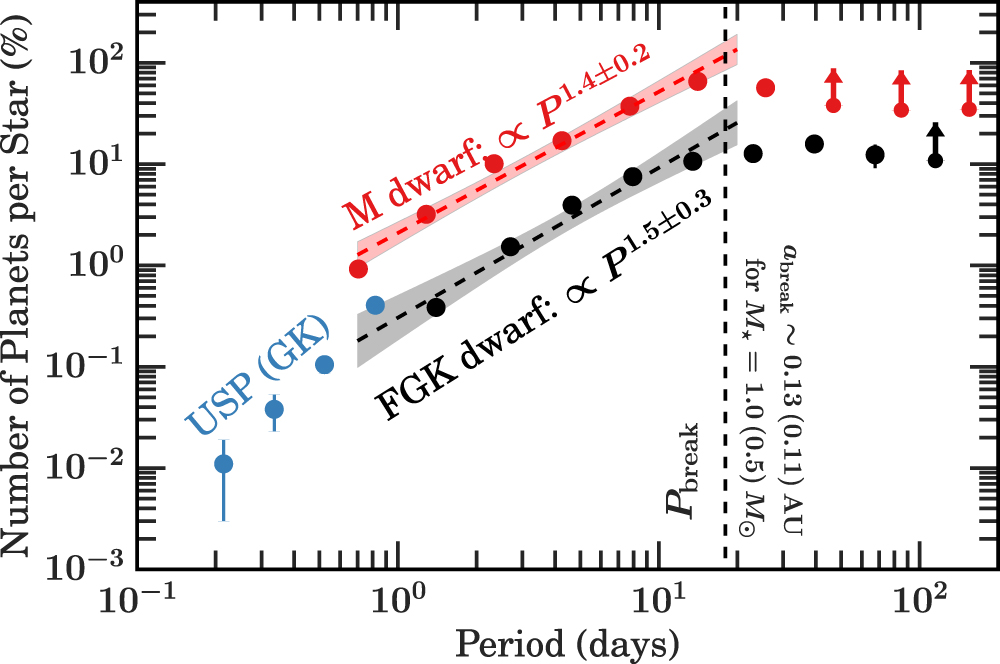
Figure 1. Occurrence rates of sub-Neptunes ( ) orbiting FGK dwarfs (Fressin et al. 2013) and early M dwarfs (Dressing & Charbonneau 2015). A distinctive break at
  days divides long-period planets at
  from their less common, short-period counterparts at
  . Strikingly, short-period planets around FGKM host stars all appear to be distributed according to
  . We also distinguish "ultra-short-period" (USP) planets at P < 1 day, using data from Sanchis-Ojeda et al. (2014). All planets are labeled according to their host star spectral types. Points without arrows correspond to sub-Neptunes larger than
  for M dwarf hosts, and larger than
  for FGK hosts. Points with arrows represent sub-Neptunes larger than
  (M dwarfs) and larger than
  (FGK dwarfs).
Download figure:
Standard image High-resolution imageThe lower occurrence rate of planets at  (hereafter "short-period" planets) may reflect a truncation of their parent disks—perhaps by the magnetospheres of their host stars (e.g., Mulders et al. 2015; see also Plavchan & Bilinski 2013). The theory of "disk locking" posits that the inner disk edge corotates with the host star in equilibrium (e.g., Ghosh & Lamb 1979; Koenigl 1991; Ostriker & Shu 1995; Long et al. 2005; Romanova & Owocki 2016). Disk locking is supported observationally by "dippers," young low-mass stars with relatively evolved disks that exhibit material lifted out of the disk midplane, presumably by magnetic torques, near the corotation radius (Stauffer et al. 2015; Ansdell et al. 2016; Bodman et al. 2016).4
The rotation periods
(hereafter "short-period" planets) may reflect a truncation of their parent disks—perhaps by the magnetospheres of their host stars (e.g., Mulders et al. 2015; see also Plavchan & Bilinski 2013). The theory of "disk locking" posits that the inner disk edge corotates with the host star in equilibrium (e.g., Ghosh & Lamb 1979; Koenigl 1991; Ostriker & Shu 1995; Long et al. 2005; Romanova & Owocki 2016). Disk locking is supported observationally by "dippers," young low-mass stars with relatively evolved disks that exhibit material lifted out of the disk midplane, presumably by magnetic torques, near the corotation radius (Stauffer et al. 2015; Ansdell et al. 2016; Bodman et al. 2016).4
The rotation periods  of stars that are 1–40 Myr old, displayed in Figure 2, range from 0.2 to 20 days, squarely in the range occupied by short-period planets. Moreover, the distribution of
  peaks near ∼10 days and falls toward shorter periods, mirroring, at least qualitatively, the decline in the planet occurrence rate at
  .5
In this paper we develop, in quantitative detail, this possible connection between disk truncation at corotation and the occurrence rate profile of short-period planets.
.5
In this paper we develop, in quantitative detail, this possible connection between disk truncation at corotation and the occurrence rate profile of short-period planets.

Figure 2. Histograms of pre-main-sequence stellar rotation periods  in clusters of various ages: the Orion Nebula Cluster (ONC, Herbst et al. 2002; Rodríguez-Ledesma et al. 2009), NGC 2362 (Irwin et al. 2008a), and NGC 2547 (Irwin et al. 2008b). Rotation periods are measured from periodic light curve variations due to starspots. For higher-mass stars (top panel), the distribution of
  for all three clusters peaks at ∼10 days and falls off at shorter periods. Lower-mass stars (bottom panel) tend to rotate faster at the same age. Older clusters harbor more rapidly rotating stars, as expected from stellar contraction. See Section 3.2 for a discussion of these trends.
Download figure:
Standard image High-resolution imagePlanets that form outside the inner disk truncation radius can be brought to the disk edge, and even transported inside it, by a variety of migration mechanisms. These include disk torques (e.g., migration types I and II; see the review by Kley & Nelson 2012), stellar tidal friction, and planet–planet gravitational interactions. We model the first two processes in this paper but not the third. Below we briefly review migration by planet–planet interactions and explain why it cannot produce the bulk of short-period sub-Neptunes.
- 1.Secular excitation of eccentricities in a multi-planet system, coupled with tidal circularization, can shrink planetary orbits and produce short-period planets (e.g., Wu & Lithwick 2011; Hansen & Murray 2015; Matsakos & Königl 2016). The sub-Neptune 55 Cnc e may have been so nudged onto its current 0.7 day orbit (Hansen & Zink 2015). But general-relativistic precession at short periods usually defeats secular forcing by perturbers less massive than Jupiter. While many short-period sub-Neptunes are members of multi-planet systems (e.g., Pu & Wu 2015; Steffen & Coughlin 2016, and references therein), their nearby companions are not typically gas giants and therefore cannot compete against general-relativistic precession. 55 Cnc e is atypical because its four neighbors range in mass from 0.2 to 5
 (where is the mass of Jupiter), creating a web of strong secular resonances.
 - 2.Violent planet–planet scatterings (i.e., close encounters) can deliver planets from large stellocentric distances to small ones where their orbits can be circularized by tides. But tidal circularization takes time, on the order of Myr to Gyr for periapse distances between 0.03 and 0.1 au. During that time, planets may collide with others and fail to attain short periods. When bodies are on eccentric and crossing orbits, encounters/mergers are more likely to occur at large rather than small distances because bodies spend less time near their periastra, and because interactions are less gravitationally focused at small distances. High-eccentricity migration of short-period sub-Neptunes is hard to reconcile with the observation that such planets are commonly found with close exterior neighbors.6


In this work we attempt to explain the observed occurrence rate profiles of short-period planets, focusing on reproducing the break period  and the shape of the decline in planet frequency at
  . We take as our starting point circumstellar disks whose inner edges are located at corotation with their host stars, drawing disk truncation periods directly from observed stellar rotation periods (i.e., Figure 2). Outside the disk truncation radius, we consider separately the possibility that sub-Neptunes migrate inward by torques exerted by residual disk gas, and the possibility that disk-driven migration is negligible, i.e., that planets form in situ. In either case, we account for orbital decay driven by asynchronous equilibrium tides raised by planets on their host stars. We examine whether tidal friction can create "ultra-short-period" planets (USPs with P < 1 day) from short-period planets, in proportions similar to those observed. Our Monte Carlo (MC) model incorporating these various ingredients is presented in Section 2. We summarize in Section 3, highlighting those areas that need the most shoring up, and venturing a few predictions.
2. MC Simulations
We construct a MC model for the occurrence rates of sub-Neptunes versus orbital period. Our goal is to identify those parameters related to disk truncation, disk-driven planet migration, and tidal inspiral that can reproduce the shapes of the observed occurrence rate profiles as shown in Figure 1.
The following Sections (2.1–2.3) detail the three steps taken to construct a given MC model.
2.1. Step 1: Draw Disk Truncation Periods from Stellar Rotation Periods
We create  disks, each truncated at its own innermost edge at period
  . The disks are assumed to be magnetospherically truncated at corotation with their host stars (i.e., we assume disk locking): each value of
  is drawn directly from an empirical distribution of stellar rotation periods
  . A given MC model utilizes rotation periods measured for one of three stellar clusters: the Orion Nebula Cluster (ONC, age of 1 Myr), NGC 2362 (5 Myr), and NGC 2547 (40 Myr). For MC models of planets around FGK dwarfs, we draw
  using stars with masses
  (upper panel of Figure 2). For MC models of planets around M stars, we do the same for stars with masses
  (lower panel of Figure 2).
2.2. Step 2: Lay Down Planets Following Either "In Situ" Formation or "Disk Migration"
Each disk is taken to contain  planets. Their initial periods—initial as in before stellar tides have acted—are decided according to one of two schemes. "In situ" formation models are very simple: the pre-tide planet periods are distributed randomly and uniformly in log period from
  to
to  days. The logarithmic spacing befits planetary systems that form by in situ, oligarchic accretion, whereby planets are separated by a multiple number of Hill radii (e.g., Kokubo & Ida 2012). Our specific choices of
  and
and  days affect only the normalization of the occurrence rate profile; this normalization is adjusted later to fit the observations (see the captions to Figures 4 through 8). The aim of this paper is to reproduce the breaks and slopes of the observed occurrence rates, not their absolute normalizations.
The alternative "disk migration" models start the same way as the in situ models, but transport planets to shorter pre-tide periods according to the Type I migration rate:

where a is a given planet's orbital radius,  is its mass, Ω is its orbital angular frequency, and TL is the combined Lindblad and corotation torque exerted by the disk on the planet (e.g., Kley & Nelson 2012):

where  is an order-unity constant calibrated from simulations (D'Angelo & Lubow 2010), and β and γ characterize an assumed power-law gas disk of surface density

and temperature

Other variables include the disk scale height  , the gas mean molecular weight μ, the mass of the hydrogen atom
  , and Boltzmann's constant k.
For simplicity, regardless of whether the host stars modeled are FGK dwarfs or M dwarfs, we fix  ,
,  K,
K,  ,
,  , and
, and  . We fix
  for FGK dwarfs and
  for M dwarfs. The errors introduced by fixing these variables are subsumed to some extent by large uncertainties in the disk parameters β,
  , and the dissipation timescale
  . We now describe and comment on our choices for these three parameters:
- 1.For a given MC model, we set β to one of three values:. If we assume that a disk's gas traces its solids (i.e., a spatially constant gas-to-solids abundance ratio), then these β-values encompass the range of quoted slopes in the literature, as inferred from observations of exoplanets comprising mostly solids: to (e.g., Hansen & Murray 2012; Chiang & Laughlin 2013; Schlichting 2014; Hansen 2015). Note that follows immediately from (this flat slope is seen at long periods in Figure 1) if the characteristic planet mass does not vary much with distance.
- 2.We experiment with two normalizations for the gas surface density at: g cm−2. These choices yield rather gas-poor disks, depleted by 3–4 orders of magnitude relative to solar-composition "minimum-mass nebulae." Such highly gas-depleted environments are motivated by the need to defeat gas dynamical friction before sub-Neptune cores can form by the mergers of protocores (Lee & Chiang 2016, their Figure 5). We assume that Type I migration proceeds normally in these gas-poor disks and discuss this assumption in the
Appendix . - 3.


Having assigned all parameters for our disk migration model, we then migrate every planet inward by integrating Equation (1) over a time interval of  (10 e-foldings of the disk gas density).
2.2.1. What Happens when Planets Migrate into the Innermost Edge
The first planet to migrate by disk torques toward the disk truncation radius will park in its vicinity—either interior to the disk edge where the last of the principal Lindblad torques peters out (Goldreich & Tremaine 1980; see also Lin et al. 1996); at the disk edge because of principal corotation torques (Tanaka et al. 2002; Masset et al. 2006; Terquem & Papaloizou 2007); or exterior to the disk edge following the reflection of planet-driven waves off the edge (Tsang 2011). In our MC model, we assume for simplicity that the first planet that can migrate by disk torques to arrive at the inner edge does so, and stays there (until step 3, after which it and all other planets move further in by stellar tides). Experiments that do not park this first planet at  but instead at
  (so that the planet is located at the interior 2:1 resonance with the disk edge) change none of our qualitative conclusions.
We have two options for the planets that subsequently follow this first parked planet. In one class of MC model ("resonance lock"; see Figure 3 for an illustration), we stop a planet when it migrates convergently into mean-motion resonance with its interior neighbor. For simplicity, we consider only 3:2 resonances (the choice of 3:2 is motivated by the observation that, of the small subset of Kepler planets located near resonances, most are situated near 3:2; Fabrycky et al. 2014). In a second class of MC model ("merged"), planets are allowed to migrate unimpeded to the innermost disk edge and assumed to merge there with the first planet. We count the merger product as a single planet, equivalent to all other planets in our final tally of planet occurrence rates (this simplification should be acceptable insofar as observed occurrence rates based on transit data are typically tallied by planet radius, which at fixed bulk density does not change appreciably when a planet doubles or triples its mass).

Figure 3. How Type I migration might play out for a system of sub-Neptunes in a disk that truncates at a period  day and whose surface density depletes exponentially with time. We assume β = 2 and γ = 1/2 for the gas disk, normalizing the surface density at 0.1 au according to the inset equation. At time t = 0,
  (gas is depleted by ∼4 orders of magnitude with respect to the solar-composition minimum-mass solar nebula). All 5 planets have equal mass (
 ) and adjacent pairs are initially spaced 14 mutual Hill radii apart (see, e.g., Figure 6 of Pu & Wu 2015; note that in our actual MC models, we randomize the initial orbital spacings). Each planet's trajectory is computed by integrating Equation (1). The innermost planet is forced to halt once it reaches the disk's inner edge. Under the "resonance lock" assumption, planets that follow the first planet are stopped once they migrate, convergently, into 3:2 resonance. The final state comprises a chain of 3 resonant planets inside 10 days, 1 non-resonant planet that has migrated to just outside 10 days (about a third of its starting period), and 1 outermost planet that has hardly moved because its migration timescale
  exceeded the disk e-folding time
  , assumed for this figure to be 1 Myr.
Download figure:
Standard image High-resolution imageThe intention behind these two flavors of MC model is to bracket the range of possible planet–planet interactions near the disk edge. On the one hand, convergently migrating planets can become trapped in a resonant chain (e.g., Terquem & Papaloizou 2007) or linger near resonances (Deck & Batygin 2015). Although observed short-period planets are generally not found in resonance (e.g., Sanchis-Ojeda et al. 2014, their Figure 8), orbital instabilities over the Gyr ages of observed systems can lead to mergers of resonant planets, transforming them into (lower multiplicity) non-resonant systems. Numerical N-body integrations of high-multiplicity systems show that resonances are preferentially unstable; non-resonant neighbors appear to destabilize otherwise stable resonant pairs (Mahajan & Wu 2014; Pu & Wu 2015, their Figure 5). Our "resonance lock" model captures mergers of destabilized resonant pairs insofar as merger products should have the same period distribution, statistically, as their progenitors.
On the other hand, planets that collect near the inner disk edge may never lock into resonances and instead collide into each other—hence our "merged" model. Given the potential complexity of planet–planet and planet–disk interactions near the disk edge (e.g., Tanaka et al. 2002; Masset et al. 2006; Tsang 2011; Deck & Batygin 2015; Liu et al. 2017)—interactions that may be modulated by the looming stellar magnetosphere (e.g., Romanova & Owocki 2016) and/or disk magnetic fields (e.g., Terquem 2003)—it would be unsurprising if planets fail in general to be captured into resonance in this messy environment.
2.3. Step 3: Apply Tidal Orbital Decay
The asynchronous equilibrium tide raised by a planet on its host star causes its orbital semimajor axis to decay at a rate

where  is the stellar radius and
  is the effective tidal quality factor (Goldreich & Soter 1966; see also Ibgui & Burrows 2009). For every planet, we integrate Equation (5) over a time interval of 5 Gyr to calculate its final "post-tide" orbital period.7
Equation (5) assumes that planets remain on circular orbits, and that planet orbital periods are shorter than the stellar rotation period (otherwise planets would migrate outward). The latter assumption becomes safer as stars age beyond the zero-age main sequence and slow their spins. Although the assumption is violated for the planets with the longest periods (say ≳ 10 days), such planets hardly migrate by tides anyway because of the steep dependence of tidal friction on a. We do not consider planet–planet interactions during tidal migration, as tides act to separate orbits: divergently migrating planets can cross resonances but do not lock into them, and the eccentricities that sub-Neptunes impart to one another when crossing resonances are small (see, e.g., Dermott et al. 1988).
is the effective tidal quality factor (Goldreich & Soter 1966; see also Ibgui & Burrows 2009). For every planet, we integrate Equation (5) over a time interval of 5 Gyr to calculate its final "post-tide" orbital period.7
Equation (5) assumes that planets remain on circular orbits, and that planet orbital periods are shorter than the stellar rotation period (otherwise planets would migrate outward). The latter assumption becomes safer as stars age beyond the zero-age main sequence and slow their spins. Although the assumption is violated for the planets with the longest periods (say ≳ 10 days), such planets hardly migrate by tides anyway because of the steep dependence of tidal friction on a. We do not consider planet–planet interactions during tidal migration, as tides act to separate orbits: divergently migrating planets can cross resonances but do not lock into them, and the eccentricities that sub-Neptunes impart to one another when crossing resonances are small (see, e.g., Dermott et al. 1988).
For FGK dwarfs, we fix  and vary
  , a range that overlaps with estimates based on observations and modeling of hot Jupiters (e.g., Matsumura et al. 2008; Hansen 2010; Schlaufman et al. 2010; Penev et al. 2012). For M dwarfs, we fix
  and vary
  . The smaller values of
  for M dwarfs are motivated by the idea that stellar tidal dissipation mostly occurs in convective zones, which are larger for lower-mass stars (see, e.g., Hansen 2012, their Figure 3).
Having computed the final periods of all planets in all disks, we tally them up to calculate model occurrence rates versus orbital period, using the same period bins as reported by the observations (Fressin et al. 2013 and Sanchis-Ojeda et al. 2014 for FGK dwarfs; Dressing & Charbonneau 2015 for M dwarfs). We construct both probability distribution functions (PDFs) and corresponding cumulative distribution functions (CDFs) to compare directly with their observational counterparts. This comparison is done by eye—we are looking for broad trends and aiming to identify, only in an order-of-magnitude sense, those regions of parameter space that are compatible with the observations. Our choices on how to normalize our PDFs and CDFs are given in the figure captions.
2.4. Results for FGK Host Stars
We begin by reviewing the results of MC models for disk migration, first omitting the effects of tidal orbital decay in Section 2.4.1 and then incorporating them in Section 2.4.2. In situ + tidal models are presented in Section 2.4.3.
2.4.1. Disk Migration without Tidal Friction
Figure 4 shows that despite the many free parameters, our disk-migration-only models give practically the same results: overprediction of the number of short-period planets at 0.5 day ≲ P ≲ 10 days, a tendency to underpredict longer-period planets at P ≳ 10 days, and a failure to capture ultra-short-period planets at P ≲ 0.5 day. Disk migration scoops out too many planets at large P to overpopulate small P.

Figure 4. Model occurrence rates (solid lines) including Type I disk migration in a dissipating nebula but excluding tidal migration. Model curves are computed using the same period bins as those reported from observations of sub-Neptunes orbiting FGK stars (Fressin et al. 2013, black points) and GK stars (Sanchis-Ojeda et al. 2014, blue points), and normalized such that their maxima match the maximum observed occurrence rate. The left panels correspond to "merged" models in which planets that migrate to the disk inner edge merge there. The right panels correspond to "resonance lock" models in which planets that migrate convergently into 3:2 resonance are locked into that resonance. At P ≲ 1 day, merged models exhibit a pile-up in the occurrence rate, while resonance lock models exhibit a sharper decline. At P ≲ 10 days, models do not differ much when disk parameters β,  , and
, and  are varied (see each panel's annotations). The distribution of disk truncation periods is drawn from the stellar rotation periods in NGC 2362 (age ∼ 5 Myr). The model curves shown here omit tidal migration and are unable to produce USPs. If we allow disk migration to
  then the models have the opposite problem of overproducing USPs. See later figures for models that include both disk and tidal migration.
Download figure:
Standard image High-resolution imageThat bins at P < 0.5 day are empty follows from  day (for NGC 2362, the stellar cluster used to make Figure 4), and our assumption that planets do not migrate past the disk truncation period
  . We have tried relaxing this assumption, allowing planets to migrate to
  (i.e., parking them at 2:1 resonance with the disk edge; see Section 2.2.1). This succeeds in creating USPs, but merely extends the problem of overproducing short-period planets (relative to the observations) to P < 0.5 day (data not shown).
The occurrence rate profiles at P ≲ 10 days appear almost identical over a wide range of disk parameters (β,  ,
,  ) because "all roads lead to Rome": various disk migration histories all end with the same outcome of planets converging onto disk inner edges, whose period distribution is fixed by the distribution of stellar rotation periods. The details of the planet distribution in the vicinity of the edge depend on what assumption we adopt: "merged" models pile up planets at P ∼ 0.5–1 day, while "resonance lock" models spread planets out more evenly in
  from ∼1–3 days (under our assumption that planets lock into 3:2 resonance; in general, for a
  resonance, the pile-up sharpens with increasing j). At longer P ≳ 10 days, there is more variation between disk models. In particular, β = 1 yields such high disk densities at large orbital radius that all planets at long periods are flushed inward by disk migration.
2.4.2. Disk Migration with Tidal Friction
Incorporating tidal inspiral into our disk migration models can yield improved fits to the occurrence rate of USPs at P ≲ 1 day. In Figure 5 we apply tidal decay to one of the disk-migration-only models shown in Figure 4 ( , β = 2, and
  Myr). From the grid of models in Figure 5, it appears that using stellar rotation periods from NGC 2362 and
  works best for reproducing USPs, either in merged or resonance lock models (middle column, blue curves).

Figure 5. Occurrence rates of planets that have undergone both disk (Type I) migration in a dissipating nebula, and tidal migration over 5 Gyr. For reference, the black solid lines include only disk migration and exclude tidal migration. As in Figure 4, we overplot the observed occurrence rates of sub-Neptunes around FGK stars with black and blue circles. All model curves utilize the same period bins as the reported observations, and are normalized such that they intersect the observed data point at P = 39.5 days. In each column, disk truncation periods are drawn from stellar rotation periods measured for a cluster of a certain age: 1 Myr for the Orion Nebula Cluster (ONC), 5 Myr for NGC 2362, and 40 Myr for NGC 2547. Irrespective of whether the innermost planets merge at the truncation radii of their disks (top panels labeled "merged") or are spaced according to mean-motion resonances (bottom panels labeled "resonance lock"), the observed occurrence rate profile for USPs (P < 1 day) can be reproduced by tidal migration, with the best fits corresponding to a stellar tidal friction parameter  and an intermediate age (NGC 2362). Note, however, how in all cases disk migration overestimates the frequency of planets with periods between 1 and 10 days.
Download figure:
Standard image High-resolution imageDrawing disk truncation periods from older clusters, which contain more rapidly rotating stars (Figure 2), produces more USPs. In the oldest cluster considered (NGC 2547 at 40 Myr), typical disk truncation periods are so short that tidal inspiral is required to reduce the number of USPs and better match observations. In the youngest cluster considered (ONC at 1 Myr), tidal inspiral is also required, but for the opposite reason: disk truncation periods here are too long and no USPs are generated without tidal migration. The case of NGC 2362 is intermediate and exhibits both behaviors.
All disk+tidal models, however, overproduce planets with periods between ∼1 and 10 days. This is the same problem as seen in disk-migration-only models (Section 2.4.1). Tidal orbital decay has too short a reach to eliminate this excess.
2.4.3. In Situ Models with Tidal Friction
Figure 6 showcases in situ MC models, with and without tidal friction. At P ≳ 3 days, these models fit the observations remarkably well, performing better than the disk+tidal migration models in this period regime. Simply assuming that sub-Neptunes are randomly distributed in their disks (in a uniform  sense) avoids the overproduction-at-short-P/underproduction-at-long-P problem introduced by disk migration.

Figure 6. Occurrence rates of planets that form "in situ" (i.e., at locations randomly and uniformly distributed in  ) and that subsequently undergo tidal migration over 5 Gyr. The format of this figure is similar to that of Figure 5, except that the bottom row of panels plots the cumulative distribution function (CDF), normalized to unity at the longest period bin (i.e., only counting planets with P ≤ 67.5 days). Tidal migration appears necessary to produce USPs at P < 1 day. By eye, best fits correspond to
  and disk truncation periods drawn from intermediate-to-late age clusters like NGC 2362 and NGC 2547. These in situ+tidal models do better than corresponding disk+tidal migration models (cf. Figure 5 and see also Figure 7) at reproducing the number of planets with periods between 1 and 10 days; at the same time, they tend to underpredict the number of USPs at P ≲ 0.5 days.
Download figure:
Standard image High-resolution imageUltra-short-period planets (USPs) can be reproduced, approximately, by tidal orbital decay of planets located near the inner edges of their disks. Drawing the shorter disk truncation periods from older clusters like NGC 2362 and NGC 2547 works best by giving planets a "head start" toward the shortest periods.
Figure 7 zooms in to directly compare one of the better fitting in situ+tide models with its disk+tide counterpart. With respect to the observations, the in situ+tide model does better than the disk+tide model at P ∼ 1–10 days by not overproducing the number of planets. But for that same reason, the disk+tide model does better than the in situ+tide model at P ≲ 1 day: disk migration generates more USPs by supplying more planets for tidal inspiral, and matches the observations at ultra-short periods more closely. Both classes of model overpredict the number of planets at P ∼ 1–3 days.

Figure 7. Zoom-in of some best-fitting disk+tidal and in situ+tidal models, selected from Figures 5 and 6, respectively. In the disk+tidal migration models (blue and cyan curves), the dissipating nebula is characterized by  . The linear scaling shown on the right emphasizes that the disk+tidal migration models overpredict the number of planets with periods between 1 and 10 days. In particular, both the "merged" and "resonance lock" models produce pile-ups just inside 10 days that are not seen in the observations. In this period range, the in situ+tidal model (red curve) better reproduces the data. But at P < 1 day, the situation reverses, as seen in the logarithmic scaling at left. Disk migration transports planets efficiently to the shortest periods where tides can bring them further in; thus, disk+tidal models tend to produce more USPs than in situ+tidal models, in better agreement with observations.
Download figure:
Standard image High-resolution image2.5. Results for M Host Stars
Figure 8 compares model occurrence rates for planets orbiting M dwarfs against observations. The best agreement is obtained for in situ+tidal models calculated by drawing  from the ONC and by adopting
  . Using these same assumptions in disk-induced migration models gives worse fits characterized by an excess of planets inside ∼10 days. Appealing to stronger tidal dissipation can remove much of this excess but simultaneously destroys USPs by shuttling them to the stellar surface.

Figure 8. Occurrence rate profiles of sub-Neptunes around M dwarfs from in situ+tidal models (top row), disk+tidal models in which planets merge at the disk edge (middle row), and disk+tidal models in which the innermost planets lock into a resonant chain (bottom row). Disk truncation radii are drawn from stellar rotation periods  measured in clusters of varying age, including the Orion Nebula Cluster (ONC, 1 Myr, left column), NGC 2362 (5 Myr, middle column), and NGC 2547 (40 Myr, right column). The rate of orbital decay by stellar tides is calculated using Equation (5) with
  and
and  . Observational data (black circles) are adopted from Figure 12 of Dressing & Charbonneau (2015). All model curves are computed using the same period bins as used in the reported observations, and are normalized such that they intersect the observed data point at 14 days. The dissipating nebula underlying the disk+tidal models obeys
  . The in situ+tidal models with
  from the ONC and with
  agree best with the observations.
Download figure:
Standard image High-resolution imageWe require a significantly smaller  to produce a best-fitting in situ+tidal model for M dwarfs (
 ) as compared to FGK dwarfs (
 ). M stars tend to rotate faster than FGK stars, so stronger tides are needed to remove the excess of planets near ∼1–2 days. The smaller
  for M dwarfs supports the idea that the bulk of stellar tidal dissipation occurs in convective zones, which are larger for lower-mass stars (e.g., Hansen 2012, and references therein).
Drawing  from clusters older than the ONC overestimates the number of planets inside 10 days, as stars spin up with age and truncate their disks at shorter periods. This effect is amplified for M stars over FGK stars because M dwarfs spin up more rapidly as they get older; see in Figure 2 how the peak of the period distribution shifts more dramatically with age for lower-mass stars. The excess population is especially difficult to remove when planets enter into and remain in a "resonance lock" near the disk edge. Resonance lock models distribute planets broadly over this period range, beyond the reach of tidal friction in M stars even for
  .
.
3. Summary and Discussion
Around FGK and M stars, sub-Neptunes appear evenly distributed at orbital periods P ≳ 10 days, but become increasingly rare toward shorter periods. Through MC population synthesis calculations, we demonstrated how this orbital architecture arises from disks truncated at corotation with their host star magnetospheres, and from orbital decay driven by stellar tidal dissipation. The dropoff in planet occurrence rate at P ∼ 1–10 days traces the distribution of planets near the inner edges of their parent disks; in turn, the distribution of disk edges reflects the distribution of stellar rotation periods in young clusters 1–40 Myr old. At the same time, despite disk truncation, planets can migrate inward to ultra-short periods (P < 1 day) by the asynchronous equilibrium tides they raise on their host stars.
We found better fits to observed occurrence rates when planets were randomly distributed in log P within their parent gas disks—as might be expected if they formed in situ—rather than brought to disk edges by disk torques. Figure 9 recaps how well our in situ+tidal models reproduce the occurrence rates of planets orbiting FGK dwarfs and early M dwarfs. However, none of our models, predicated either on in situ formation or disk migration, fit the data perfectly; the former do better at large P while the latter do better at short P. In situ models might yield improved fits if we had a more accurate theory for tidal orbital decay, or if the distribution of disk inner edges were broader than we have assumed. Such broadening could be achieved by relaxing our assumption that disks truncate exactly at corotation, or by issuing sub-Neptunes from disks with a range of dissipation timescales. For example, the disk truncation period could be drawn from a mix of stellar rotation periods characterizing both the young Orion Nebula Cluster and the older NGC 2547 (but see Section 3.2). It is also possible that the stellar rotation period distributions we have used are not entirely representative. The cluster Cep OB3b has a similar age (4–5 Myr) as NGC 2362, but its median rotation period for M dwarfs may be ∼1.6 times longer, assuming its low-mass stars are correctly identified as such (Littlefair et al. 2010).

Figure 9. In situ planet formation in disks truncated at corotation by host star magnetospheres, in combination with tidal migration, can reproduce the observed occurrence rates of sub-Neptunes. Black and blue points represent observations of planets orbiting FGK dwarfs by Fressin et al. (2013) and Sanchis-Ojeda et al. (2014), respectively, and red points represent observations of planets orbiting early M dwarfs by Dressing & Charbonneau (2015). Points without arrows correspond to sub-Neptunes larger than  for M dwarf hosts, and larger than
  for FGK hosts. Points with arrows represent sub-Neptunes larger than
  (M dwarfs), and larger than
  (FGK dwarfs). Our best-fitting model for FGK hosts uses stellar rotation periods drawn from NGC 2362 at an age of 5 Myr, and
  . Our best-fitting model for M-type hosts uses rotation periods drawn from the Orion Nebula Cluster at an age of 1 Myr, and
  . These same models are plotted in Figures 6–8, but we display them again here for ease of viewing.
Download figure:
Standard image High-resolution imageBelow we explore how our theory might be extended to bear on other observed properties of short-period sub-Neptunes and their host stars, attempting where possible to make predictions for future observations.
3.1. Orbital Spacings of USPs
We have shown in this paper the essential role tides play in creating USPs. Another line of evidence pointing to the influence of tides can be found by examining planetary orbital spacings. Because tidal orbital decay generally proceeds more quickly at smaller periods, interplanetary spacings should be stretched out more (in a fractional sense) at small P than at large P. Just such a signature is observed: USPs are more widely spaced than their longer-period counterparts (Steffen & Farr 2013). In Figure 10 we demonstrate how orbital spacings widen preferentially at the shortest periods because of tides. Comparison of our model with observations shows only qualitative agreement; the empirical data (gray circles and orange line) suggest that tidal friction in reality is more effective at drawing planets apart than our constant- theory allows (blue curves). A better theory for tidal friction, one incorporating dynamical tides and the evolution of stellar spin and structure, is needed to better reproduce the data (see, e.g., Bolmont & Mathis 2016, and references therein).

Figure 10. Observational evidence for how stellar tidal friction widens separations between planets most effectively at the shortest orbital periods. Each gray circle represents the orbital spacing, measured in mutual Hill radii  , between the two shortest-period transiting planets ("tranets") in a given multi-tranet system, and is plotted against the shorter period of the pair. These data, downloaded on 2016 December 5 from the NASA Exoplanet Archive and based on Quarters 1–16 of the Kepler space mission, include only sub-Neptunes (
 ). In calculating mutual Hill radii, we assumed all tranets to have
  . The median observed spacing, plotted as a thick orange solid line, is fairly constant at P > 2 days, but grows dramatically toward shorter periods. Such behavior is expected, qualitatively, from tidal migration. The blue lines indicate theoretical orbital spacings between adjacent pairs of
  planets after 5 Gyr of tidal orbital decay; the central star on which tides are raised is assumed to have a mass
  , radius
  , and tidal quality factor
  . From bottom to top, the theory curves correspond to pairs of planets separated initially (before tides act) by 5, 15, ..., 95
  , and each is plotted against the final (post-tide) orbital period of the inner member of a pair.
Download figure:
Standard image High-resolution image3.2. Trends with Stellar Mass
Mulders et al. (2015) point out how the sub-Neptune occurrence rate breaks at  days regardless of whether the host star is of spectral type F, G, K, or M. In our theory, the break and dropoff at shorter periods reflect the distribution of stellar spin periods
  . We can reproduce the invariance of
  by drawing
  from a distribution that does not vary with stellar mass. The Orion Nebula Cluster (ONC) provides such a spin distribution, which peaks at ∼10 days irrespective of whether the stars are ∼1 M⊙ or ∼0.3 M⊙ (compare the top and bottom panels of Figure 2). Drawing
  from the ONC implies that planets emerge from disks that dissipate over the ONC age of ∼1 Myr. One problem with our ONC-based models is that they underestimate the number of USPs, particularly around FGK stars (left column of Figure 6); not enough stars rotate with periods faster than a day. USPs are produced more easily around older, more rapidly rotating stars (middle and right columns of Figure 6), but these have
  distributions that do vary with stellar mass (Figure 2) and therefore have trouble reproducing the invariance of
  (note how the model break period in the middle and the right columns of Figure 8 misses the observed break period by a factor of 5). Simultaneously fitting both USPs and their longer-period counterparts near the break is a challenge, requiring improvements in our understanding of disk truncation and tides.
There is also room for improvement for observations: the USP occurrence rates from Sanchis-Ojeda et al. (2014) appear systematically offset from the Fressin et al. (2013) data at longer periods; see how the blue points in Figure 9 appear to be shifted higher than the black points. Whether this offset is real or an artifact of combining two different data sets is unclear; removal of the offset would ameliorate if not solve the problem noted above with our ONC-based models. A uniform analysis is needed to measure planet occurrence rates from ∼0.1 to >10 days, not just for FGK stars but also for M stars.
Detecting and characterizing planets around main-sequence A stars is the next frontier. The invariance of  with respect to stellar spectral type may not extend to A stars. Compared to T Tauri stars, Herbig Ae stars are observed to be faster rotators, with typical spin periods of ∼1 day (Hubrig et al. 2009; Alecian et al. 2013). It follows that their gas disks should truncate at shorter periods.8
We therefore predict the occurrence rate of sub-Neptunes to break at a correspondingly short period
with respect to stellar spectral type may not extend to A stars. Compared to T Tauri stars, Herbig Ae stars are observed to be faster rotators, with typical spin periods of ∼1 day (Hubrig et al. 2009; Alecian et al. 2013). It follows that their gas disks should truncate at shorter periods.8
We therefore predict the occurrence rate of sub-Neptunes to break at a correspondingly short period  day around A stars, as compared to
  days for FGKM stars. This shift in
  between high-mass and low-mass stars is illustrated in Figure 11. The break around A stars might occur at even shorter sub-day periods, as our spin period data for A stars are taken from stellar magnetic field studies whose samples are biased to include more slowly rotating stars (Hubrig et al. 2009; Alecian et al. 2013). Figure 11 also shows that tidal inspiral does not much alter the period break for A stars for
  . These larger values of
  are motivated by main-sequence A stars lacking outer convective envelopes (see, e.g., Mathis 2015, their Figure 4). A caveat to our prediction that sub-Neptunes around A stars exhibit a shorter
  is that we have so far discussed only disks of gas, not disks of solids—and sub-Neptunes are primarily composed of solids. Dust disks around A stars may not extend down to periods of ∼1 day because of sublimation (e.g., Dullemond & Monnier 2010, their Figure 7). Nevertheless, larger solids (planetesimals orders of magnitude larger than dust grains) are more resistant to vaporization and can drift, aerodynamically or otherwise, through gas disks toward their inner edges, assembling into planets there.

Figure 11. Pre-main-sequence A stars rotate faster than pre-main-sequence FGK or M stars (top panel), and we therefore expect that the planet occurrence rate for A stars breaks at a shorter period  than that for FGKM stars (bottom panel). Rotation periods of 1–10 Myr old Herbig Ae stars are taken from Table 7 of Hubrig et al. (2009), updated using Table 2 of Alecian et al. (2013). These rotation periods were calculated from spectroscopically determined stellar radii and rotation velocities de-projected using disk inclinations; the latter were measured either from resolved disk images or inferred from the line profile shapes of the Mg ii or Hα emission lines. Pre-tide and post-tide models, all assuming in situ formation, are shown in the bottom panel as solid and dashed lines, respectively; for FGKM stars, we use the model parameters that yield the best agreement with observations (ONC and
  for M; NGC 2362 and
  for FGK). To account for the shorter main-sequence lifetime of higher-mass stars, we apply tidal migration around A stars for only 1 Gyr (versus 5 Gyr for FGKM stars). For planets around A stars, within a plausible range of
  (and taking
  and
and  ), we find that
  day, considerably shorter than the period break for FGKM stars (∼10 days). There is a weaker secondary break at ∼1 day around FGK dwarfs that reflects the bimodal distribution of rotation periods for stars in this mass range (Figure 2; see also Bouvier 2007 and references therein).
Download figure:
Standard image High-resolution imageWe thank Kevin Covey, Trevor David, Dan Fabrycky, Brad Hansen, Brian Jackson, Dong Lai, Jing Luan, Gijs Mulders, Ruth Murray-Clay, James Owen, Ilaria Pascucci, Roman Rafikov, Saul Rappaport, Fred Rasio, Hilke Schlichting, Jason Steffen, Scott Tremaine, and Josh Winn for helpful discussions. An anonymous referee provided an exceptionally thoughtful and encouraging report. This research has made use of the NASA Exoplanet Archive, which is operated by the California Institute of Technology, under contract with the National Aeronautics and Space Administration under the Exoplanet Exploration Program. E.J.L. was supported in part by the Berkeley Fellowship and by NSERC of Canada through PGS D3. E.C. acknowledges support from NASA and NSF.
Appendix: Migration in Gas-poor Disks
In our MC models with disk-induced Type I migration, we chose gas surface densities so low that the planet mass  exceeds, by roughly two orders of magnitude, the local disk mass
  . For the planet to migrate inward, it must lose its angular momentum to the disk. Because
  , one might worry that the need to transfer so much angular momentum from the planet to the local disk would severely perturb the latter, so much so that the planet would cease to undergo normal Type I migration. Perhaps the planet stops migrating altogether; or perhaps it opens a deep and wide gap and migrates at the Type II rate set by disk viscosity.
Even when  , Type I migration might still prevail in disks with large enough viscous stresses to prevent the opening of gaps and to transport angular momentum—both the planet's and the disk's—outward to distances of a few au.9
For our chosen disk parameters, we find that as long as the Shakura–Sunyaev viscosity parameter
, Type I migration might still prevail in disks with large enough viscous stresses to prevent the opening of gaps and to transport angular momentum—both the planet's and the disk's—outward to distances of a few au.9
For our chosen disk parameters, we find that as long as the Shakura–Sunyaev viscosity parameter  , super-Earths of mass
  will not open gaps at short periods (Duffell & MacFadyen 2013; Fung et al. 2014). Furthermore, for the disk depletion time to be as long as
  Myr, the disk must be able to transport mass and momentum across large distances extending well beyond the innermost regions where short-period planets reside. For example, assuming
  (as per above), the viscous drainage time of the disk,
  (for viscosity ν), is as long as
  Myr only for
  . The mechanism of disk transport remains unclear, but the magneto-rotational instability and magnetized winds are perennial candidates, especially in the hot and well-ionized innermost disk, and perhaps also beyond, under gas-poor conditions (see, e.g., Wang & Goodman 2017).
Even if migration is not Type I, its exact form should have little bearing on our disk+tide migration models at orbital periods shorter than ∼20 days. As we demonstrated in Section 2.4.1, the period distribution of close-in planets is determined largely by the distribution of stellar rotation periods, which sets disk truncation periods. In our disk+tide models, it does not much matter how planets are transported to disk edges, as long as they arrive there. We reiterate that our in situ+tide models, which omit disk migration altogether, give overall better fits to the observations, especially at P > 1 day.
Footnotes
- 3
The Trappist-1 planetary system (Gillon et al. 2017, and references therein) is hosted by a late M dwarf.
- 4
Stellar magnetic fields measured from Zeeman broadening do not correlate well with field strengths predicted from magnetospheric truncation (see the review by Bouvier 2007 and references therein). However, relaxing the assumption that the stellar field is a pure dipole brings theory into closer agreement with observations (see, e.g., Cauley et al. 2012, and references therein).
- 5
All stellar rotation periods
shown in Figure 2 are measured from periodic light curve variations driven by starspots. Photometric retrieval of is biased against young and especially active T Tauri stars exhibiting irregular variability caused by strong and unsteady disk accretion. This bias is small—Herbst et al. (2002) estimate that their sample of periodic stars is incomplete by 8%–15%—and its effect on our analysis should be still more muted because we take the orbital architecture of planets to be established during the latest stages of disk evolution, when the disk has largely (but not completely) dissipated (see Section 2.2). As for the clusters NGC 2362 and NGC 2547, Irwin et al. (2008a, 2008b) find, respectively, that their surveys are complete down to and across all measured rotation periods. - 6
By contrast, high-eccentricity migration of hot Jupiters is compatible with the observation that they have distant, not close, exterior companions (Bryan et al. 2016).
- 7
The models shown in this paper assume that the host star radius is fixed in time and ignore the pre-main-sequence contraction phase during which the star is still distended and the tidal decay rate (which scales as
) is correspondingly enhanced. We experimented with relaxing this assumption and found that accounting for the full time evolution of stellar radius changes negligibly the final planet occurrence rate profiles. The pre-main-sequence phase lasts only ∼20–60 Myr for 1–0.5 M⊙ stars, and is typically much shorter than the orbital decay timescales of planets that do not fall onto the star. - 8
Herbig Ae stars can have magnetospheres. They are observed to have typical surface magnetic field strengths of ∼100 G (see, e.g., Hubrig et al. 2009, their Figure 10). For disk accretion rates of 10−7–10−10 M⊙ yr−1 around a star of mass
and radius , magnetospheric truncation radii range between ∼1 and 4 stellar radii. - 9
By contrast, in inviscid disks, the inability of the disk to carry away the planet's angular momentum presents a serious problem for Type I migration. A "migration feedback" torque can stall planets in low-mass, laminar disks (Ward & Hourigan 1989; Ward 1997; Rafikov 2002; Li et al. 2009; Yu et al. 2010; Fung & Chiang 2017).


