


Abstract
We examine the possibility that icy super-Earth mass planets, formed over long timescales (0.1–1 Gyr) at large distances (∼200–1000 au) from their host stars, will develop massive H-rich atmospheres. Within the interior of these planets, high pressure converts CH4 into ethane, butane, or diamond and releases H2. Using simplified models that capture the basic physics of the internal structure, we show that the physical properties of the atmosphere depend on the outflux of H2 from the mantle. When this outflux is  molec cm−2 s−1, the outgassed atmosphere has a base pressure of ≲1 bar. Larger outflows result in a substantial atmosphere where the base pressure may approach 103–104 bar. For any pressure, the mean density of these planets, 2.4–3 g cm−3, is much larger than the mean density of Uranus and Neptune, 1.3–1.6 g cm−3. Thus, observations can distinguish between a Planet Nine with a primordial H/He-rich atmosphere accreted from the protosolar nebula and one with an atmosphere outgassed from the core.
Export citation and abstract BibTeX RIS
1. Introduction
There has recently been a great deal of speculation about the possibility of a large planet at a distance of several hundred astronomical units from the Sun (Trujillo & Sheppard 2014; Batygin & Brown 2016; Brown & Batygin 2016; Sheppard & Trujillo 2016). If this planet forms (1) in the inner solar system and (2) rapidly enough (≲1–10 Myr) to capture hydrogen and helium from the protosolar nebula, it will probably have a composition similar to the ice giants Uranus and Neptune. Deriving the cooling history and predictions for the atmospheric structure may then rely on extensions of models developed for ice giants (Fortney et al. 2016; Ginzburg et al. 2016; Linder & Mordasini 2016).
In an alternative model, an icy Planet Nine forms in situ (Kenyon & Bromley 2016). For the long growth times expected (≳0.1–0.3 Gyr), Planet Nine is then a volatile-rich super-Earth composed solely of icy planetesimals. With negligible hydrogen or helium accreted from the protosolar nebula, any atmosphere would have to be outgassed from the interior.
Predicting the atmospheric structure of an icy Planet Nine requires a new model for the cooling history. Studies of water-rich super-Earths show that the identity of the chemical species that can outgas into the atmosphere and their corresponding fluxes strongly depend on (1) the high- and low-pressure crystal structures formed in the mantle, (2) solubility both in the liquid and solid phases, (3) the details of the mantle dynamics, and (4) surface–atmosphere interaction (Levi et al. 2013, 2014).
The purpose of this paper is to construct a basic model for the atmosphere of an icy super-Earth at 250–750 au from a solar-type star. Developing a self-consistent model that follows the change in structure of the planet as it accretes and evolves is a major undertaking beyond the scope of this study. Instead, we break the problem up into smaller, more manageable pieces, each of which is designed to deal with a different aspect of the problem. In Section 2, we summarize results for the model of Kenyon & Bromley (2016), which establishes the accretion rate expected for this case. In Section 3, we apply this accretion rate to estimate the temperature profile inside the planet using a model adapted from Malamud & Prialnik (2016). The high temperatures derived in this calculation imply that most of the planet differentiates to a rock core and an ice shell. With this result established, we use a structure model adapted from the work of Helled et al. (2015), which uses more careful equations of state and explicitly allows for the pressure dissociation of methane and the release of hydrogen. This analysis yields an estimate of the hydrogen reservoir in the planet. In Section 4, we quantify the abundance of hydrogen in a secondary outgassed atmosphere surrounding a water-rich super-Earth.
This analysis suggests plausible outcomes ranging from a thin atmosphere with a pressure of less than 1 bar to a thick atmosphere with a pressure of several hundred bars. In Section 5, we compare this range of structures to those expected for an ice giant, consider the expected abundance ratio of methane to hydrogen, discuss observations that can distinguish between the two possibilities, and outline possible improvements to our approach. We conclude in Section 6 with a brief summary.
2. Super-Earth Mass Planets at 250–750 au
Kenyon & Bromley (2016) and Bromley & Kenyon (2016) outline options for placing a super-Earth mass planet in the outer solar system (see also Stern 2005; Li & Adams 2016; Mustill et al. 2016). In the simplest model, the protosolar nebula produces five gas giant planets at 5–20 au. Gravitational interactions among these gas giants scatter one into the outer solar system. If a massive protosolar nebula extends to 200–500 au, dynamical friction between the scattered planet and the gaseous nebula circularizes the orbit of the planet at 300–600 au (Bromley & Kenyon 2016). As a variant of this model, physical processes in another planetary system produce a low-mass gas giant orbiting at several hundred astronomical units. A close encounter between the solar system and this other planetary system allows the Sun to capture this planet on an eccentric orbit at 300–600 au (Kenyon & Bromley 2004; Li & Adams 2016; Mustill et al. 2016). Although it is much more likely that either of these mechanisms results in an ice giant on a wide orbit, it is possible that the planet could be scattered or captured before it accretes hydrogen and helium from the nebula. The planet is then a large ball of ice and rock.
Kenyon & Bromley (2015, 2016) explore models where massive planets grow in situ from a massive ring of icy solid material leftover from the formation of the solar system (see also Stern 2005; Kenyon & Bromley 2008). If the ring is composed of a mono-disperse swarm of 1–100 cm objects, the time for agglomeration processes to produce a super-Earth mass planet is (Kenyon & Bromley 2015)

where M0 is the initial mass in solids and a is the orbital distance from the Sun. Within the 4.5 Gyr lifetime of the solar system, this process allows growth of massive icy super-Earths at 100–300 au. The growth of icy planets beyond 300 au requires a very massive ring or a formation timescale much longer than 4.5 Gyr.
If the ring of icy pebbles cools dynamically, a gravitational instability can produce one or more protoplanets with radii of 100 km or larger (Kenyon & Bromley 2016, and references therein). Figure 1 summarizes the evolution of these protoplanets accreting from a ring of icy 1 cm pebbles at 750 au. After roughly 100 Myr of slow growth, the protoplanets undergo a phase of "runaway growth" where their masses increase from 10−6  to roughly 0.1
  . As they grow in mass, these protoplanets stir up the leftover pebbles to higher orbital eccentricity, which slows growth. During the next 1–2 Gyr, destructive collisions among the leftovers generates a sea of 0.1–1 mm fragments. Over time, collisional damping among the fragments circularizes their orbits. Protoplanets can then accrete the fragments rapidly, leading to a second phase of runaway growth where protoplanets reach super-Earth masses.
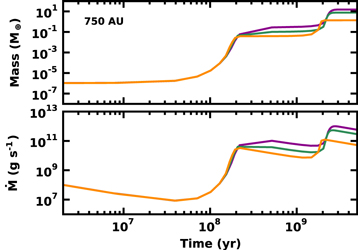
Figure 1. Evolution of icy planets at 750 au. Upper panel: mass of the largest object as a function of time for calculations with one (violet curve), two (green curve), and four (orange curve) 100 km objects accreting from a sea of 1 cm pebbles. Lower panel: same as in the upper panel, but for the accretion rate onto the largest objects.
Download figure:
Standard image High-resolution imageNumerical calculations with a variety of starting conditions suggest that systems of one to two protoplanets are much more likely to produce 10–15  planets than systems of four or more protoplanets. The timescale to reach super-Earth masses is (Kenyon & Bromley 2016)

where  2–2.5. This in situ growth time for protoplanets (100 Myr to 1–2 Gyr) is much longer than the 5–10 Myr lifetime of the protosolar nebula (Williams & Cieza 2011). Thus, these protoplanets never accrete gas from the protosolar nebula and are simply balls of ice and rock.
In either the in situ formation or the scattering scenario, a massive Planet Nine on an orbit with an eccentricity of  and a semimajor axis of
  clears away icy pebbles and planetoids along its orbit over millions of years. Although the architecture of the outer solar system provides some constraints on the mass and orbit of a putative Planet Nine (e.g., Batygin & Brown 2016; Brown & Batygin 2016, etc.), these results are somewhat controversial (Shankman et al. 2017). If Planet Nine is discovered, the properties of its atmosphere will provide important clues about formation mechanisms (e.g., Fortney et al. 2016). Thus, we consider constraints based on models where Planet Nine is originally a ball of ice with negligible atmosphere.
3. Size of the H2 Reservoir
Planetesimals at 100–1000 au, which agglomerate into an icy Planet Nine are probably composed of a mixture of rock and ice. To derive an estimate of the composition, we adopt the relative elemental abundances of Lodders (2010) and assume that the most abundant rock-forming elements, Fe, Mg, and Si, combine with O to form rocky material. Any remaining O then forms water; leftover C and N form CH4 and NH3, respectively. All of the leftover H forms H2, while the remaining abundant elements, He and Ne remain as atomic noble gases. At the low temperatures (∼20 K) relevant to this region of the solar system, CH4, NH3, and H2O are frozen. Thus, any planetesimal is composed of rock plus these three ices. Experiments show that CH4 under pressure dissociates to more complex hydrocarbons and releases hydrogen. The exact pressure of dissociation depends on temperature (Hirai et al. 2009; Kolesnikov et al. 2009; Gao et al. 2010; Lobanov et al. 2013). To estimate the pressures and temperatures inside the planet, we need to provide a model of the interior.
A proper calculation of the interior structure of an icy super-Earth requires (1) an accretion rate, (2) the energy released by accretion, gravitational compression, and radioactive decay, and (3) an accurate treatment of material and energy transport throughout the planet. Developing such a code is beyond the scope of this work. For the purpose of estimating the expected structure and temperatures, we adapted a 1D evolution code that was originally written for much smaller bodies (Prialnik & Merk 2008; Malamud & Prialnik 2015, 2016). This code computes the material and energy transport inside a growing body composed of water ice in a rock matrix that is in hydrostatic equilibrium. Energy of compression is calculated using a Birch–Murnaghan equation of state with variable coefficients. Further details can be found in the references cited. This model is not strictly applicable to the situation we are considering since the pressures in the interior are too high to be properly modeled by the Birch–Murnaghan EOS. In addition, it is likely that the planetesimals accreting onto the planet will have rocky pebbles embedded in an ice matrix rather than the other way around. Despite these issues, the resulting internal structure and heat release should be similar to that derived from a more detailed calculation, and can be used to posit the initial physical and thermal structure.
For the accretion rate of Kenyon & Bromley (2016), the central temperature of the planet rises to  K. Under these conditions, most of the interior ice melts and differentiates from the rock, giving a rock core surrounded by a liquid water layer. Temperatures in the outermost layer are considerably lower, and it does not differentiate completely. Instead, this outermost layer is ice-rich, with a porosity increasing toward the surface. The details of the temperature structure, thickness of the different layers, porosity, etc., depend on a number of parameter choices, and a qualitative diagram of the assumed initial physical and thermal structure is given in Figure 2. In what follows, we simply assume that the planet is completely differentiated and use the pressures derived from hydrostatic equilibrium to estimate the amount of hydrogen that can be produced from the dissociation of methane trapped in the water ice.
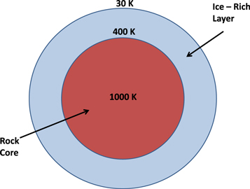
Figure 2. Illustration of the approximate initial physical and thermal structure of the planet.
Download figure:
Standard image High-resolution imageAnother important result from modeling the accretion is that the temperature at the boundary between the rock core and the ice mantle is ∼400 K. For such low temperatures, the data of Gao et al. (2010) show that methane dissociates to ethane (C2H6) plus hydrogen above 95 GPa. Above 158 GPa (287 GPa), methane dissociates to butane C4H10 plus hydrogen (carbon/diamond plus hydrogen). If it can be transported to the surface, the hydrogen formed during this dissociation is volatile enough to form an atmosphere even at the lowest temperatures expected for Planet Nine.
Using the accretion history from Section 2, this analysis suggests that a primordial Planet Nine formed in situ consists of a rock core surrounded by an ice mantle. The ice will be a mixture of H2O, CH4, and NH3. Since we are primarily interested in the behavior of the CH4, we have included the NH3 together with the H2O and used the equation of state of water to represent the mixture. NH3 is a relatively small fraction of the total, and the abundances of the different species are uncertain, so this approximation seems acceptable.
To estimate the magnitude of the hydrogen reservoir, we adapted the models of Helled et al. (2015) to compute the pressures inside a planet composed of a rock core surrounded by a mantle with a mixture of H2O and CH4. Where the pressure is high enough, the CH4 dissociates to ethane, butane, or carbon (depending on the pressure) and releases a corresponding amount of H2. We stress that we do not compute a detailed model of Planet Nine's interior; rather, we estimate the amount of H2 available for outgassing.
For the rock core, we use the equation of state for SiO2. The equations of state for SiO2, H2O, CH4, and C4H10 are taken from the SESAME tables. There are no good data for the equation of state of C2H6 at high pressure; experiments by Goncharov et al. (2013) indicate that its density is approximately a factor of 1.2 higher than that of methane over a large range of pressure. Since C2H6 is a relatively minor component, we modeled it by simply multiplying the density of CH4 by 1.2. The pressure–density relation inside the planet was calculated assuming constant temperature. Isotherms of 50 and 500 K gave nearly identical results, so this assumption is reasonable for estimating the hydrogen reservoir.
For solar abundances, we expect mass fractions of  ,
,  , and
, and  . We have also run cases where the ratio
  was kept constant but a lower methane abundance was assumed. We considered
  , 0.05, and 0.01. The results are shown in Figure 3. As can be seen from the figure, a planet with a mass of
  or more will have high enough pressures in the water–methane layer to produce H2 by CH4 dissociation. For the case of
  and a
and a  planet, enough hydrogen is produced to provide an atmosphere with a pressure of 430 bar at its base. It should be noted that the Lodders (2010) H2O to rock ratio of 1.33 is significantly lower than the older value of 2.13 derived from the abundance tables of Anders & Grevesse (1989). Planets with a higher H2O to rock ratio have higher pressures in the H2O–CH4 mantle, which lead to more methane dissociation and a larger reservoir of H2. Thus our models provide a lower limit to the size of that reservoir.

Figure 3. Pressure (solid curves) at the base of the hydrogen atmosphere, and its equivalent mass (dashed curves), as a function of planetary mass for CH4 mass fractions of 0.24 (purple curve), 0.1 (green curve), 0.05 (red curve), and 0.01 (blue curve) if all the available internal hydrogen is assumed to be outgassed.
Download figure:
Standard image High-resolution image4. Constraints on the Extent of a Secondary Outgassed H2 Atmosphere
If hydrocarbon processing in the deep ice mantle releases vast quantities of H2, building a rich H2 atmosphere requires transport to the outer edge of the planet. The efficiency of this transport depends on the ability of H2 to become incorporated into the water ice matrix.
The phase behavior of the binary H2–H2O system was recently studied, mainly for purposes of examining novel hydrogen storage techniques. Up to a pressure of 0.36 GPa, a sII clathrate hydrate of H2 is stable, which, when filled to capacity, contains 48 hydrogen molecules per 136 water molecules in every unit cell (Lokshin et al. 2004). At 0.36 GPa, there is a structural transformation to a phase that is stable up to about 0.8 GPa. It is referred to as the new phase by Strobel et al. 2011. The nature of this structure is not yet clear, but X-ray diffraction (Strobel et al. 2011) and molecular simulations (Smirnov & Stegailov 2013) indicate several possibilities. Smirnov & Stegailov (2013) suggested various structures, which were tested by looking at the minimum of the free energy and by examining their stability using classical molecular dynamics. These authors suggested either a unit cell composed of 6 water molecules and 3 hydrogen molecules or a unit cell composed of 12 water molecules and 4 hydrogen molecules.
At room temperature and approximately 0.8 GPa, the H2–H2O system transforms from clathrate to filled ice of phase C1, with 36 water molecules for every 6 hydrogen molecules. At 2.3 GPa, a phase transformation to filled ice C2 occurs with equal abundances of water and hydrogen molecules. This latter phase is stable up to 40 GPa at room temperature (see Strobel et al. 2011, and references therein). Ab initio simulations for zero temperature suggest that, at 38 GPa (including a zero point correction), a new phase (C3) with a composition of H2O:2H2 becomes stable and remains stable to 120 GPa (Qian et al. 2014). The high stability of C3 is attributed to the very low Bader volume of hydrogen in this structure resulting in a highly dense crystal.
It is not yet known whether the crystal structures just mentioned are also stable at the temperatures prevailing in the deep ice mantle of a possible Planet Nine at 500–1000 au. However, the results do suggest that H2 is highly soluble in high pressure water ice structures. Therefore, a non-negligible partition coefficient between any internal H2 reservoir and an overlying high pressure water ice matrix is reasonable. This structure will result in the outward transport of internally produced H2 along with the water ice convection cell.
We wish to investigate the atmosphere generated from this H2 flux. To estimate whether such an atmosphere is dynamically stable and how its structure depends on the surface geology and the phase diagram of the binary H2–H2O system, we begin by looking at the phase diagram of the sII clathrate hydrate of H2 (see Figure 4). The equilibrium of this phase with water ice Ih is difficult to explore experimentally due to the very slow kinetics of formation (Struzhkin et al. 2007). Few experiments trying to identify the three-phase curve of this phase with respect to ice Ih and liquid water exist (e.g., Mao & Mao 2004; Lokshin & Zhao 2006).
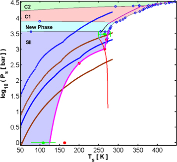
Figure 4. Blue and brown curves are the pressure and temperature relations at the planetary solid surface, i.e., at the base of the H2 atmosphere, for different conditions at unit opacity. Brown curves assume an effective temperature of 30 K at unit opacity where the pressure is taken to be either 0.1 bar (solid brown curve) or 1 bar (dashed brown curve). Blue curves assume an effective temperature of 20 K at unit opacity where the pressure is taken to be either 0.1 bar (solid blue curve) or 1 bar (dashed blue curve). The solid magenta curve is a guide to the eye, going through the published data points for the three-phase curves: sII Clathrate-ice Ih-H2 fluid and sII Clathrate-liquid water–H2 fluid. Green data points with their associated errors are from Mao & Mao (2004). Red circles are data points from Lokshin & Zhao (2006). Hollow blue circles are data points from Vos et al. (1993), Dyadin et al. (1999a, 1999b), Antonov et al. (2009), and Efimchenko et al. (2009). The solid red, cyan, black, purple, and dashed purple curves are the pure water ice Ih, ice III, ice V, ice VI, and ice VII melt curves, respectively. The different stability fields for the various phases in the H2O–H2 binary solution are represented by the shaded areas.
Download figure:
Standard image High-resolution imageIn Figure 4, we also plot the relation between the temperature, Ts, and pressure, Ps, at the base of an H2 atmosphere (see blue and brown curves). To derive this relation, we need to tie the temperature at depth to the temperature at the top of the atmosphere. If we scale the effective temperature of a planet at a distance a from the Sun by

then the effective temperature of the planet is  at 750 au and
  at 250 au. For a hydrogen atmosphere, the optical depth is approximately (Lewis & Prinn 1984)

where P is the pressure in bars, d is the thickness of the atmospheric layer in kilometers, which we approximate by the scale height, and α is the thermal IR absorption coefficient for pressure-induced absorption by H2. With  km−1 amg−2,
  corresponds to a pressure of
  , which we take to be the pressure corresponding to the effective temperature.3
Other values suggested in the literature for unit opacity in an H2 atmosphere are 0.2 bar (Wordsworth 2012) and around 1 bar (Birnbaum et al. 1996). Heat release by radioactive decay could raise the effective temperature to some 30 K. Since the optical depth is proportional to
, which we take to be the pressure corresponding to the effective temperature.3
Other values suggested in the literature for unit opacity in an H2 atmosphere are 0.2 bar (Wordsworth 2012) and around 1 bar (Birnbaum et al. 1996). Heat release by radioactive decay could raise the effective temperature to some 30 K. Since the optical depth is proportional to  , raising the effective temperature by a factor of two would raise the pressure at
  by the same factor. This is well within the range given in the literature. In Figure 4, we solve for various unit opacity conditions.
Once the atmosphere is optically thick, we expect the region below to follow an adiabat (as suggested in Stevenson 1999). For a pure hydrogen atmosphere this adiabat can be computed from the data in the SESAME tables by integrating the thermodynamic relation  , where E is the energy per unit mass of material, and V is the corresponding volume per unit mass. This approach gives us a relation between the surface temperature and pressure.
From Figure 4, we are able to identify a transition point, which depends on the conditions adopted for unit opacity. This point marks the thermodynamic condition where the surface pressure provided by the H2 atmosphere becomes less than the dissociation pressure of the sII clathrate hydrate of H2, if one goes in the direction of increasing temperature. For example, if unit opacity is at 20 K and 0.1 bar, the transition point is at about 269 K and approximately 1720 bar. If unit opacity is at 30 K and 0.1 bar, the transition point is at about 159 K and approximately 54 bar.
This relation has an interesting dynamical consequence. In Figure 5, we show a low-temperature section of Figure 4, to the left of the transition point (for an example adiabat). Let us imagine a water-rich planet for which the conditions at the base of its H2 atmosphere fit point A in Figure 5. Since this point is above the dissociation pressure of the sII clathrate hydrate of H2, the hydrogen from the atmosphere reacts with the water ice surface to form clathrate hydrate. The driving force to form this clathrate phase exists until the H2 pressure in the atmosphere reduces to that of point B. However, the reduction in the abundance of hydrogen in the atmosphere also cools the surface of the planet, driving the conditions at the base of the atmosphere toward point C. The new H2 pressure at the surface is again higher than the dissociation pressure for the sII clathrate hydrate of H2 for the new and lower surface temperature, and the process continues.
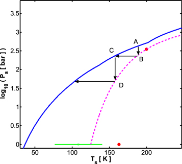
Figure 5. Low-temperature section of Figure 4. The solid thick blue curve is the pressure and temperature relation at the planetary solid surface, i.e., at the base of the H2 atmosphere, for unit opacity conditions of 20 K and 0.1 bar. The dashed magenta curve is a guide to the eye, going through the published data points for the three-phase curve hydrate-ice Ih-H2 fluid. The green data point with its associated error is from Mao & Mao (2004). Red circles are data points from Lokshin & Zhao (2006). See the text for an explanation of arrows and letters.
Download figure:
Standard image High-resolution imageThe lack of low-temperature experimental data for the dissociation pressure of the sII clathrate hydrate of H2 means that we cannot determine at what point this process of atmospheric H2 removal terminates. However, we may tentatively conclude that there are two dynamically stable end scenarios for the hydrogen atmosphere. One is a poor sub-bar H2 atmosphere if the transition point is not reached, and the other is a H2 atmosphere more massive than the transition point pressure if the system is perturbed or otherwise set at conditions beyond the transition point. We note that this transition point pressure is relatively low compared to what potential internal reservoirs of H2 can provide. In addition, the mechanism for the deposition of the H2 atmosphere into clathrates may be slow. Therefore, even after billions of years such an atmosphere may survive. Finally, it is possible that an outgassing flux of H2 may be established that can counteract this deposition mechanism.
We can estimate the efficiency of the proposed atmospheric H2 removal mechanism. Experiments on the enclathration of CH4 and CO2 show that clathrate formation is initially relatively fast during the stage of a micron-scale surface reaction, and then slows down considerably as clathrate promoters have to diffuse through the outer enclathrated layer in order to reach fresh ice Ih (Staykova et al. 2003; Genov et al. 2004). Therefore, the depth from the surface that can participate in the enclathration of atmospheric H2 is

where D is the diffusion coefficient of H2 in the water matrix, and t is the time that has elapsed. Thus the number of moles of water taking part in this process is

Here, Rp is the planet's radius,  is the mass density of water ice Ih, and
  is the molar weight of water. In a fully occupied sII clathrate hydrate of H2, a unit cell composed of 136 H2O molecules entraps 48 H2 molecules (Lokshin & Zhao 2006). The number of moles of H2 that can be taken out of the atmosphere after time t is

The relation between the surface pressure due to the H2 atmosphere and the mass,  , of this atmosphere is

where g is the surface acceleration of gravity. After rearranging we have

where  is the molar weight of diatomic hydrogen.
The self-diffusion coefficient of H2 in its hydrate water matrix is the subject of ongoing research (e.g., Nagai et al. 2008; Trinh et al. 2015). For our purposes, we require the diffusion coefficient at low temperatures where tunneling of H2 is important. Alavi & Ripmeester (2007) found that the H2 diffusion coefficient for crossing the hexagonal face of a sII clathrate hydrate large cage is 10−4 cm2 s−1, while crossing a pentagonal cage face corresponds to a diffusion coefficient of 10−7 cm2 s−1. We can estimate the effective self-diffusion coefficient by treating the sII clathrate as a multicomponent system, where we assume each cage type is a "different" component. According to Weertman & Weertman (1975), this results in an average diffusion coefficient of
where we use the fact that each sII unit cell is composed of 8 large cages (first component) and 16 small cages (second component).
Let us consider a planet with a mass of 15  , for which we calculate a gravitational surface acceleration of g = 1570 cm s−2. After t = 1 Gyr, the removal mechanism can deposit approximately 4 bar of atmospheric H2 into clathrates. This can be translated into an average critical flux:
Here  is the number of H2 molecules equivalent to the 4 bar deposited in t = 1 Gyr. For the planets we model, if they are below the transition point, having an H2 outgassing flux higher (lower) than the critical flux means their atmospheres would become richer (poorer) in H2 with time.
As mentioned in the Introduction, we consider the case of a water-rich super-Earth forming at large heliocentric distances. The slow accretion rate (Kenyon & Bromley 2016) means that it will not reach a mass large enough to capture an H/He envelope from the surrounding nebula before that nebula dissipates. If our water-rich super-Earth experiences a subcritical H2 outflux, it probably has a negligible H2 atmosphere. Clearly, this scenario results in a distinctive mass density and atmospheric composition, different than those of a classical ice giant similar to Neptune or Uranus. However, a supercritical outgassing flux of H2 enriches the atmosphere with time. To learn whether this evolution leads to a structure similar to an ice giant, we now examine the thermal profile and dynamics of the planetary ice crust and upper mantle, and how these evolve as the atmosphere is enriched with H2.
In Levi et al. (2014), we have developed a model for the planetary crust and underlying convection for a water-rich super-Earth. In this model, we solve for the case of a stagnant lid and a small viscosity contrast. We truncate the thermal conductive profile assumed for the crust by looking for the depth where the Rayleigh number reaches its critical value. Then we follow an adiabat into the planet. We refer the reader to Levi et al. (2014) for a thorough explanation of the technique used. Here we will only discuss the changes we have made to this model in its current application.
To be consistent with the analysis of the previous section, we consider the crust and upper mantle to have an ice composition of H2O and CH4, with a mole ratio of

The CH4 forms a sI clathrate hydrate, for which the H2O to CH4 mole ratio is  , assuming full occupancy of the clathrate cages. The excess H2O forms pure Ih water ice. This view is corroborated by experiments following the succession of phases with pressure in the H2O–CH4 system (Hirai et al. 2001; Loveday et al. 2001; Ohtani et al. 2010). The fraction of the ice volume occupied by the sI CH4 clathrate hydrate is

where Vns is the total volume of the sI CH4 clathrate hydrate (i.e., the non-stoichiometric crystal) in the upper ice mantle and  is the total volume of the pure water ice Ih. After several algebraic steps one can show that

Here  and
and  are the molar masses of CH4 and H2O respectively. The mass densities of the appropriate pure water ice and non-stoichiometric phases are
  and
and  respectively.
The composite mass density is

We approximate the isobaric heat capacity of the composite using the rule of mixtures:

where Cnsp and  are the isobaric heat capacities of the non-stoichiometric sI CH4 clathrate hydrate phase and of water ice Ih, respectively.
The thermal conductivity of our assumed composite ice mantle is  . This composite may be approximated as a continuous pure water ice Ih within which small non-stoichiometric sI CH4 clathrate hydrate grains are embedded. The thermal conductivity of such a composite was solved for by Maxwell (Bird et al. 2007), and for our case has the following form.

In the last relation,  is the thermal conductivity of water ice Ih. The thermal conductivity of the non-stoichiometric sI CH4 clathrate hydrate phase is
  . Therefore, the thermal diffusivity of the upper ice mantle is

The volume thermal expansivity of our composite material is  . There are various suggestions in the literature for relating the composite expansivity to that of the individual phases composing it. The rule of mixtures and Turner's formula confine the composite expansivity from above and below respectively (Schapery 1968; Karch 2014):
where  is the bulk modulus of water ice Ih, and Kns is the bulk modulus of the non-stoichiometric sI CH4 clathrate hydrate. We will adopt Turner's formula, making our adiabatic profile steeper. This means more H2 is required in the atmosphere in order to increase the surface temperature, if the adiabat is to cross the melt curve of ice Ih.
The thermodynamic data for the sI CH4 clathrate hydrate phase was given in detail in Levi et al. (2014). The mass density, isobaric heat capacity, and volume thermal expansivity for water ice Ih are taken from Feistel & Wagner (2006). The thermal conductivity of water ice Ih is taken from Slack (1980). The bulk modulus for water ice Ih is taken from Helgerud et al. (2009).
Lastly, we discuss the choice we have made for the viscosity. Durham & Stern (2001) suggested values for the effective viscosity due to dislocation creep, for planetary-type strain rates. These are an extrapolation over several orders of magnitude in the strain rate. In Levi et al. (2014), we have suggested a model for the Newtonian creep in sI CH4 clathrate hydrate, which is a function of the grain size. In Figure 6, we compare between different models for the viscosity. Above approximately 200 K, it seems that dislocation creep is not as active as diffusion creep. Also, varying the grain diameters in our diffusion creep model (see Levi et al. 2014) between 200–800 μm spans reasonable values for the viscosity in our ice crust and upper mantle when compared with the other viscosity models.
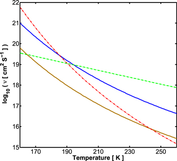
Figure 6. Kinematic viscosity at a reference pressure of 1000 bar. Dashed green curve is the dislocation creep model suggested by Durham & Stern (2001) for water ice Ih, for planetary-type strain rates. Dashed–dotted red curve is the average model for the viscosity of water ice Ih from Spohn & Schubert (2003). Solid blue curve is the Newtonian viscosity for sI CH4 clathrate hydrate from Levi et al. (2014) for grain diameters of 800 μm. Solid brown is the same model but assuming grain diameters of 200 μm.
Download figure:
Standard image High-resolution imageAgain, we assume a planet with a mass of 15  and a surface gravitational acceleration of 1570 cm s−2. With the rock mass fraction given in the previous section, we can estimate the heat released due to radioactive decay (see Equation (23) in Levi et al. 2014). This gives a surface heat flux of 46 erg cm−2 s−1. Starting from an estimated surface temperature of 20–30 K, we find our planet will be of type III of the four planetary types defined by Fu et al. (2010; see illustration in Figure 7).
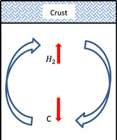
Figure 7. Planetary crust overlies a large-scale convection cell, capable of breaking the crust. In the convection cell, CH4 is dragged inward, where under high pressures it dissociates and releases H2. This hydrogen may be transported outward and reach the atmosphere. See also the type III planet in Fu et al. (2010).
Download figure:
Standard image High-resolution imageSince the surface temperature is lower than the melt temperature for water ice Ih, a solid crust forms. As discussed in Fu et al. (2010), for an ice mantle with no asthenosphere, and in Levi et al. (2014) for an ice mantle with an asthenosphere, a non-partitioned ice mantle convection cell would likely apply a high enough stress at the base of the crust to break it apart. Breaking the planetary crust exposes fresh deep ice to the surface conditions. This should result in the outgassing of H2. If H2 outgassing flux is kept supercritical, the atmosphere would become richer in hydrogen with time, thus increasing the temperature at the outer solid surface of the planet, Ts. This increase in the surface temperature shifts the temperatures along the planetary crust and upper mantle to higher values as well. Increasing the surface temperature enough may drive the deep thermal profile across the melt curve of water ice Ih, forming a subterranean ocean. The planet now attains a type II structure (see illustration in Figure 8). However, this depends on the conditions at unit opacity in the H2 atmosphere.
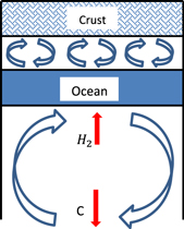
Figure 8. Planetary crust terminates with the initiation of small-scale convection, overlying a subterranean ocean. The small-scale convection cannot break the crust apart. Therefore, hindering any outgassing of H2 out into the atmosphere. See also the type II planet in Fu et al. (2010).
Download figure:
Standard image High-resolution imageIn Figure 9, we plot the minimum amount of H2 in the atmosphere required to shift the planet into a type II stratification model. As an example for the system's behavior, we assume an effective temperature of 20 K and a pressure of 0.1 bar for the unit opacity conditions in the atmosphere. Assuming an ice matrix richer in CH4 (i.e., larger η) means the composite has more sI CH4 clathrate hydrate. Because the thermal conductivity of clathrates is lower than that for ice Ih, the more clathrates in the composite, the higher the temperature increase along the crust, before reaching convective instability. Therefore, a lower surface temperature (i.e., less H2 in the atmosphere) is sufficient to transform the planet into a type II water-rich planet. In addition, the larger grain size results in a higher viscosity and thus a thicker crust. In the crust, the temperatures rise steeply with depth, hence a thicker crust means that less H2 in the atmosphere is needed in order to cross the melt curve of ice Ih.
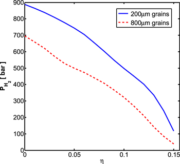
Figure 9. Minimal pressure of atmospheric H2 required to transform a type III stratified water-rich super-Earth into a type II stratified planet. η is the CH4 to H2O mole ratio of our assumed ice matrix. The solid blue curve is for our viscosity model, assuming a grain size of 200 μm, and the dashed red curve is for a grain size of 800 μm. Unit opacity conditions in the atmosphere are taken here to be 0.1 bar with an effective temperature of 20 K.
Download figure:
Standard image High-resolution imageFor the type II planetary stratification of Figure 8, we estimate the stress applied by the small-scale convective layer on the overlying crust in the following way. The maximum velocity in the small-scale convection cell is approximately

where Ra is the Rayleigh number and d is the thickness of the small-scale convective layer, between the crust and the subterranean ocean. The basal stress is

where ν is the kinematic viscosity. The stress acting to fracture the crust is thus

where dcr is the thickness of the crust.
We find that increasing η from 0 to 0.15 results in d increasing from 7 to 11 km. The crust, in general, has a thickness ranging from 1.5 to 3 km. The Rayleigh number changes by two orders of magnitude over this range of η. The stress σ falls in the range of 10−2–10−1 MPa. This is less than the tensile strength of ice Ih (1.8 MPa at 233 K, Hobbs 2010) and for sI CH4 clathrate hydrate (0.2 MPa at room temperature, Jung & Santamarina 2011). Therefore, the crust probably cannot be broken apart by the underlying small-scale convection. As a consequence, any further outgassing of internal H2 will be hindered, and the values for the pressure of atmospheric H2 given in Figure 9 represent the likely maximum values.
The ability to transition into a type II planet depends on the composition of the crust (i.e., η) and the conditions adopted for unit opacity in the atmosphere. The likely formation of a subterranean ocean may be attributed to the fact that, while the temperature increases inward along the conductive crust, the melt temperature of ice Ih decreases with increasing pressure. For lower effective temperatures or higher unit opacity pressures, conditions at the bottom of an H2 atmosphere can miss the triple point of ice Ih-ice III-liquid water. Beyond this triple point, the melt temperature of high pressure ice polymorphs increases with increasing pressure, thus rendering the formation of a subterranean ocean less likely. In such a case, the planet remains a type III planet, maintaining the ability to outgas internal H2, and possibly forming a rich H2 atmosphere on the order of 104 bar. This behavior is shown in the left panel in Figure 10, where we used  as an example, and varied the unit opacity pressure in the range of 0.1–1 bar. As is seen in the figure, having less CH4 in the crust lessens the probability for a subterranean ocean, and the ability of the atmosphere to isolate itself from the planetary inner workings.
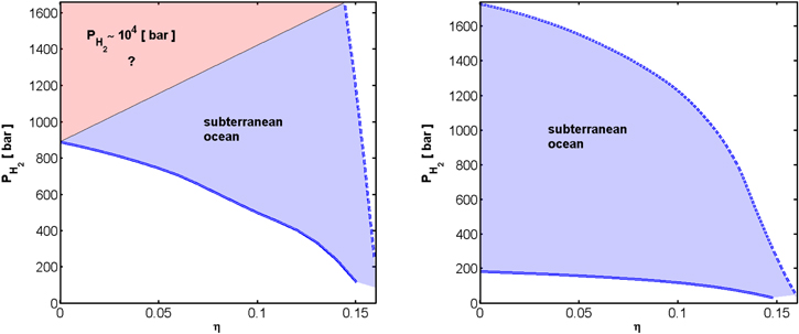
Figure 10. Here we plot the effect of varying the pressure at unit opacity for a pure H2 atmosphere, assuming an effective temperature of 20 K (left panel) and an effective temperature of 30 K (right panel). Thick solid blue curves are for a unit opacity pressure of 0.1 bar. For this value of the unit opacity pressure, for every crustal composition, from pure water ( ) to pure SI CH4 clathrate hydrate (
 ) a subterranean ocean forms, truncating any further outgassing of H2 into the atmosphere. For the effective temperature of 20 K, this curve is also the thick solid blue curve in Figure 9. For higher values of the unit opacity pressure (e.g., 1 bar, thick dashed blue curves) and for an effective temperature of 20 K, there will be a value for η below which it will no longer be possible to form a subterranean ocean. As a result, for a supercritical flux of H2, the internal reservoir of H2 may outgas into the atmosphere.
Download figure:
Standard image High-resolution imageIn the right panel in Figure 10, we have adopted  as an example, and varied the unit opacity pressure in the range of 0.1–1 bar. As is seen in this panel, the conditions at the bottom of the H2 atmosphere never miss the triple point of ice Ih-ice III-liquid water, and thus a subterranean ocean always forms. For this higher effective temperature, the internal reservoir of H2 cannot outgas completely into the atmosphere. The unbreakable crust truncates the atmosphere at a value of no more than ∼1000 bar base pressure of H2.
5. Discussion
Our analysis suggests that the pressure in the mantle of an icy super-Earth formed in situ at 250–750 au is sufficient to liberate H2 from methane. Radial transport of this H2 yields an outgassed atmosphere with a pressure of ≲1 bar to ≳100 bar. Even if the entire hydrogen reservoir of  is outgassed, however, the mean density of a 15
  icy super-Earth has a fairly small range, 2.4–3.0 g cm−3. Reducing the surface pressure of hydrogen by two orders of magnitude decreases the thickness of the atmosphere by five scale heights (∼100–500 km depending on the atmospheric temperatures) without substantially changing the radius of the bulk of the planet and increasing the expected mean density by less than 10%. Despite the potentially large atmosphere, the mean density is significantly larger than the mean density of Uranus (1.27 g cm−3) or Neptune (1.64 g cm−3). Thus, it is possible to distinguish a Planet Nine formed in situ from one which accreted gas from the protosolar nebula.
Deriving the true underlying structure of a real Planet Nine beyond 250 au requires measurements of the mass and radius. Two approaches can place limits on the radius: (1) fits of model atmospheres (e.g., Fortney et al. 2016) to multi-wavelength observations of the emitted flux and (2) occultations of background stars. Estimates for the mass rely on (1) the derivation of log g from the model atmosphere or (2) the identification of a satellite and direct measurement of its period and semimajor axis.
Although straightforward, these measurements may be challenging. Measuring the spectral energy distribution beyond 2 μm requires a Planet Nine that is bright enough for detection with JWST. Occultation observations need a Planet Nine within a field sufficiently dense with reasonably bright stars. Based on HST observations of Pluto (e.g., Brozović et al. 2015, and references therein), satellite detection seems unlikely.
Fortney et al. (2016) outline several likely possibilities for the 0.1–100 μm spectrum of a classical ice giant at ∼600 au. For the pressures expected from outgassing, the gross details of the spectrum from an icy super-Earth are probably similar. If the atmosphere is thin, surface reflectance may yield absorption features of various ices. For a thicker atmosphere, most of the gaseous methane freezes out. The spectrum of an ice giant is then dominated by Rayleigh scattering at short wavelengths, with possible features from clouds, pressure-induced H2–H2 absorption, and methane absorption at longer wavelengths. If these features exist and yield an accurate log g, then it may be possible to derive the mean density from log g and a radius inferred from the broadband spectrum.
Estimating the amount of methane and other volatiles in the outgassed atmosphere of an icy super-Earth requires an accurate assessment of outgassing and freeze-out. Although quantifying these requires a molecular-scale and macro-scale analysis of the inner workings of the icy planet, it may be possible to place some constraints on the abundance of atmospheric CH4. If any icy super-Earth with no atmosphere has a surface temperature of about 20–30 K, only H2 is volatile. If the outflux of H2 is supercritical (see Section 4) a more substantial H2 atmosphere builds with time. The surface temperature increases. When the surface temperature is roughly 50 K, CH4 adsorbed onto the surface water ice turns volatile (see adsorption timescales in Levi & Podolak 2011). Deposits of solid CH4 are also volatile. The extent of these surface CH4 reservoirs is not known and requires further research. As surface temperatures continue to increase, the kinetics of sI clathrate hydrate of CH4 accelerates. Therefore, the dissociation of the latter phase becomes an important mechanism potentially determining the abundance of atmospheric CH4.
If sI clathrate hydrates of CH4 become available to the surface, we can derive an approximate atmospheric abundance of CH4 as long as it is a trace constituent of the atmosphere. We set the planetary surface temperature from a pure H2 atmosphere and assume the CH4 content independently attains its clathrate hydrate dissociation pressure. In Figure 11, we present the atmospheric CH4/H2 mole ratio and the atmospheric pressure of H2 as a function of the planetary surface temperature. We assume unit opacity is at 0.1 bar and an effective temperature of 20 K. For lower effective temperatures or higher unit opacity pressures, more H2 is required in the atmosphere to maintain the same surface temperature. Therefore, the mole ratio of Figure 11 is an upper bound value for these cases.

Figure 11. CH4 to H2 mole ratio in the atmosphere (solid blue curve), and the atmospheric pressure of H2 (dashed green curve) vs. the surface temperature. Unit opacity is taken to be at 0.1 bar and 20 K. For higher unit opacity pressures or lower effective temperatures (i.e., temperature at unit opacity) the mole ratio given here is an upper bound value.
Download figure:
Standard image High-resolution imageTo test the assumption that atmospheric CH4 does not contribute substantially to the surface temperature, we use the results of Pavlov et al. (2003). They showed that increasing the abundance of atmospheric CH4 from 1.7 to 100 ppm increases the surface temperature by 12 K. Since the number density of the greenhouse gas in the atmosphere is the relevant parameter, we convert the above to  K cm3 molec−1. For a surface temperature of 115 K (corresponding to 70 bar of H2, for the above unit opacity parameters) the contribution of CH4 to the surface temperature is about 10%. Thus, our estimate of the CH4/H2 mole ratio is good up to
  K. The additional effect of CH4 as a greenhouse gas implies that less H2 is needed than derived here to reach surface temperatures appropriate for the formation of a subterranean ocean.
This analysis suggests that the atmospheric methane abundance might probe the underlying structure of Planet Nine. Although it is necessary to build much more comprehensive internal structure calculations of (1) ice giants with H–He atmospheres and (2) icy super-Earths with outgassed atmospheres, it might be possible to relate the atmospheric abundance of CH4 and other volatiles to the structure of the solid–gas boundary and the deeper internal structure of the planet. Aside from applications to Planet Nine, these analyses might eventually be used to probe the structures of icy exoplanets far from their host stars.
6. Summary
When icy planets grow at 250–1000 au from a solar-type star, they reach super-Earth masses too late to accrete H–He gas from a circumstellar disk. However, high pressure in the mantle of these planets converts CH4 into ethane, butane, or diamond. For planets with masses exceeding 5  the hydrogen released during this conversion can reach the surface and produce an atmosphere with a base pressure of several hundred bars.
For simplified models of the internal structure, the conditions at the base of the atmosphere favor clathrate hydrate formation, where the atmospheric hydrogen is locked in the solid water lattice. When the outflux of H2 is smaller than the critical rate of roughly 1010 molec cm−2 s−1, the outgassed atmosphere is then dynamically stable for a small base pressure ≲1 bar. Supercritical outflows can establish a substantial hydrogen atmosphere where the base pressure may approach a maximum level of 103–104 bar.
The atmospheric structure of icy planets with supercritical outflows of H2 depend on the chemical composition of the ice crust and the conditions at unit opacity. In icy planets closer to their host stars (effective temperature ∼30 K) or with ice crusts richer in clathrate hydrate promoters (lower thermal conductivity) are more likely to have a subterranean ocean. This ocean probably prevents fractures in the outer crust, restricting outgassing of internal hydrogen. The base pressure in this picture is probably a hydrogen atmosphere of a few hundred bars.
In the atmospheres of icy planets at larger distances from their host stars (effective temperature ∼10 K) or with more pure ice crusts, the hydrogen greenhouse effect may produce temperatures and base-pressures larger than the triple point of ice Ih-ice III-liquid water. A subterranean ocean is then much less likely. With no restrictions on the applied stress on the crust, it is much easier for internal hydrogen to outgas into the atmosphere. The atmospheric pressure may then reach a maximum level of ∼104 bars.
Observations can test these conclusions. Together with more comprehensive calculations of the internal structure, measurements of the gas-phase abundances of CH4 and other H-rich molecules can probe the atmospheric properties of Planet Nine. In a more basic test, Planet Nine candidates with outgassed H2 atmospheres should have much larger mean density than those with He-rich atmospheres accreted from the protosolar nebula. Several types of data, including broadband spectroscopy, and occultations, can constrain the mean density and yield insights into the origin of any massive planet in the outer solar system.
We wish to thank Prof. Dimitar Sasselov for his helpful suggestions. We further wish to thank our anonymous referee for valuable comments.
Footnotes
- 3

