


Abstract
We present measurements of the singly ionized helium-to-hydrogen ratio ( ) toward diffuse gas surrounding three ultracompact H ii (UCH ii) regions: G10.15-0.34, G23.46-0.20, and G29.96-0.02. We observe radio recombination lines of hydrogen and helium near 5 GHz using the GBT to measure the
  ratio. The measurements are motivated by the low helium ionization observed in the warm ionized medium and in the inner Galaxy diffuse ionized regions. Our data indicate that the helium is not uniformly ionized in the three observed sources. Helium lines are not detected toward a few observed positions in sources G10.15-0.34 and G23.46-0.20, and the upper limits of the
  ratio obtained are 0.03 and 0.05, respectively. The selected sources harbor stars of type O6 or hotter as indicated by helium line detection toward the bright radio continuum emission from the sources with mean
  value 0.06 ± 0.02. Our data thus show that helium in diffuse gas located a few parsecs away from the young massive stars embedded in the observed regions is not fully ionized. We investigate the origin of the nonuniform helium ionization and rule out the possibilities (a) that the helium is doubly ionized in the observed regions and (b) that the low
  values are due to additional hydrogen ionizing radiation produced by accreting low-mass stars. We find that selective absorption of ionizing photons by dust can result in low helium ionization but needs further investigation to develop a self-consistent model for dust in H ii regions.
Export citation and abstract BibTeX RIS
1. Introduction
The existence of a diffuse ionized gas in the Galaxy is evident from a variety of observations (Hoyle & Ellis 1963; see review by Haffner et al. 2009). This gas, referred to as the warm ionized medium (WIM), is now considered to be one of the major components of the interstellar medium (ISM). The WIM has been primarily studied using optical emission lines. These studies show that the local electron density of the WIM is in the range of 0.01–0.1 cm−3 and emission measures are typically ≲10 pc cm−6 (Haffner et al. 2009). In or near the disk of the inner Galaxy, optical lines suffer strong extinction, and hence the distribution of the ionized gas has been studied in the radio frequency regime. In particular, low-frequency (≲2 GHz) radio recombination line (RRL) observations have detected diffuse ionized regions (DIRs) with local density in the range of 1–10 cm−3 and emission measure ≲1000 pc cm−6 (Lockman 1976; Anantharamaiah 1986; Roshi & Anantharamaiah 2000; Alves et al. 2015). It is generally thought that both WIM and DIRs are ionized by massive stars. To maintain ionization, the WIM and the DIR together require about 80% of the ionizing radiation from all OB stars in the Galaxy (Mezger 1978; Murray & Rahman 2010). Thus, the WIM and DIR form an energetically important component of the ISM.
The WIM in the Galaxy has been shown to have low  number density ratios from optical line observations (≲0.027; Reynolds & Tufte 1995; see also Haffner et al. 2009). Here
  is the number density of singly ionized helium (He), and
  is that of ionized hydrogen (H). RRL observations toward DIRs have provided an upper limit on
  of ∼0.013 (Heiles et al. 1996; Roshi et al. 2012). Ionization of both these components of the ISM is thought to be due to UV photons from O6-type or hotter stars that leak out of H ii regions (Mezger 1978; see also Anderson et al. 2011; Luisi et al. 2016, for observational evidence of photon leakage from H ii regions). However, if stars hotter than ∼O6 are the primary ionization sources of the DIR and the WIM, the ratio
  should be close to that of the actual He/H abundance ratio of ∼0.1 (see Draine 2011, Table 15.1 and Section 15.5). This is because (1) ≤18% of the ionizing photon flux from O6 or hotter stars can fully ionize He in the ionized H region; and (2) the ionization cross sections for photons more energetic than the ionization potentials of H and He decrease with energy proportional to (hν)−3, resulting in greater mean-free paths for the highest-energy photons and expected "hardening" of the radiation field with distance from the source of ionization. Thus, the low
  ratios in the WIM and DIR are not understood.
There are at least two important issues related to the low helium ionization in the diffuse regions. First, the observed  ratio toward several H ii regions harboring O6 or hotter stars is lower than the cosmic abundance of helium (Shaver et al. 1983). The mean value of the
  ratio obtained toward such H ii regions is 0.08, indicating the presence of 20% neutral helium. The possible effects that can produce lower helium ionization include (a) selective absorption by dust (Mezger et al. 1974; see Section 5) and (b) line blanketing in the atmosphere of the O stars (see, e.g., Martins et al. 2005). Second and possibly even more problematic is how the ionizing UV photons escape through the H ii ionization fronts that surround hot O stars and the surrounding DIRs of compact H ii regions. In particular, are the
  ratios significantly decreased in their passage to the WIM? This is obviously a function of how clumpy and dusty the ISM is in the neighborhood of massive star formation regions. Although these two are important issues, the main motivation of this investigation is to determine whether the
  ratios are systematically decreased in ionized gas surrounding the earliest stages of massive star-forming regions.
Lyman continuum radiation leaking out of H ii regions ionizes gas in its immediate vicinity, as well as at large distances from the H ii region. The collection of ionized gas surrounding compact H ii regions, referred to as envelopes of H ii regions, in the inner Galaxy forms the DIR (Anantharamaiah 1986). The hierarchical structures in the molecular cloud/ISM produce similar morphology at different physical scales and at early stages of star formation. For example, many ultracompact H ii (UCH ii) regions are known to have extended, diffuse ionized gas—referred to as envelopes of UCH ii regions or UCH ii envelopes—associated with them (Garay et al. 1993; Kurtz et al. 1999; Kim & Koo 2001; see also Churchwell 2002). UCH ii regions are ionized by massive stars that are still embedded in their natal molecular cloud, thus representing a very early stage of star formation. The morphology of UCH ii regions and their envelopes is similar to that of compact H ii regions and the DIR. The emission measure of these envelopes is typically ≳ a few times 103 pc cm−6, an order of magnitude larger than the emission measure of the DIR. The envelopes of UCH ii regions absorb more than 65% of the ionizing radiation from the embedded stars (Kim & Koo 2001), which is comparable to the percentage of UV photons absorbed by the DIR. Thus, observing He RRLs from higher emission measure diffuse gas surrounding UCH ii regions may provide a clue to resolving the He ionization problem in the DIR. In Section 2 we describe the selection of sources for observation and discuss their properties. The observations and data analysis are discussed in Section 3. Our main results are presented in Section 4, and a discussion of the results is given in Section 5. A summary of the main results is given in Section 6. Appendices
2. Source Selection
A systematic study of continuum and RRL emission toward 16 UCH ii regions was done by Kim & Koo (2001). They detected diffuse, extended emission toward 14 UCH ii regions in their sample. The similarity of the LSR velocity of hydrogen RRLs from the UCH ii regions and the diffuse gas suggests that the H ii region and the diffuse component are associated (see Section 4.1 for further discussion on velocity structure based on our data set). This association is also suggested by the continuum morphology of these sources. The continuum emission from UCH ii regions and their envelope was used to estimate the Lyman continuum photon flux required to maintain ionization. This Lyman continuum photon flux is used to estimate the required stellar spectral type. The spectral types for the 14 UCH ii regions range from O4 to O9. We selected three sources (G10.15-0.34, G23.46-0.20, and G29.96-0.02) with embedded stars of type O5.5 or earlier for helium RRL observations. H ii region models with a single ionizing star suggest that the helium and hydrogen Strömgren spheres will overlap for these sources. Hence, helium is expected to be singly ionized in the envelope of the selected UCH ii regions.
VLA 21 cm images of the three selected sources G10.15-0.34, G23.46-0.20, and G29.96-0.02 are shown in Figures 1–3, respectively. These images are from the data obtained by Kim & Koo (2001) and have an angular resolution of ∼40'' × 20''. We show Spitzer three-color images of the three targets in Figures 4–6, with GLIMPSE 3.6 and 8.0 μm data in blue and green (Benjamin et al. 2003; Churchwell et al. 2009) and MIPSGAL 24 μm data in red (Carey et al. 2009). The red MIPSGAL emission is from warm dust grains spatially coincident with the ionized gas in H ii regions. The green GLIMPSE 8.0 μm emission is dominated by polycyclic aromatic hydrocarbons (PAHs) in the photodissociation regions (PDRs). A brief description of the selected sources is given below, and a summary of their properties is given in Table 1.
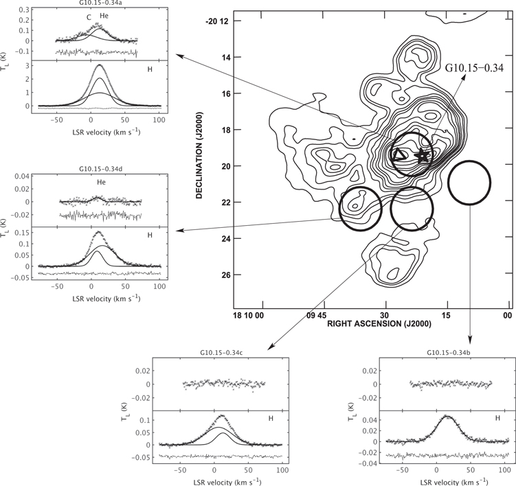
Figure 1. 21 cm continuum image (Kim & Koo 2001) of the G10.15-0.34 region (top right). The contour levels are (1, 3, 5, 10, 15, 20, 30, 40, 60, 80, 100, 150, 200, 250, 300) × 10−2 Jy beam−1. The observed positions are indicated by the continuum image, with circles of radius the size of the GBT beam (2 5). The observed spectra (indicated by crosses), the Gaussian line components (solid line), and the residual spectra (dotted line) are also shown in the figure. The position of the UCH ii region G10.15-0.34 is indicated by a star. The center of the NIR observing region that has identified four O5.5-type stars (see text) is indicated by a triangle.
Download figure:
Standard image High-resolution image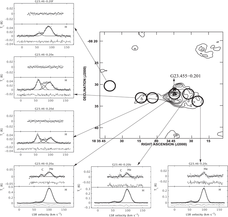
Figure 2. Same as Figure 1, except for the source G23.46-0.20. The position of the UCH ii region G23.455-0.201 is indicated by a star. The position of the IR source G23.437-0.209 (see text) is indicated by a triangle.
Download figure:
Standard image High-resolution image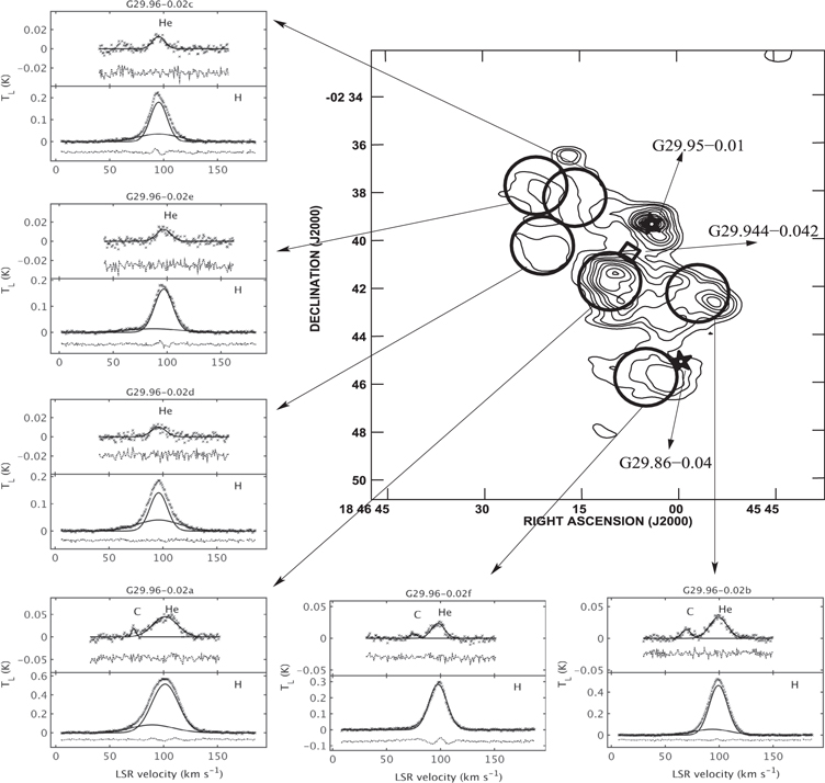
Figure 3. Same as Figure 1, except for the source G29.96-0.02. The positions of the UCH ii region G29.95-0.01 and the 12 GHz methanol source G29.86-0.04 are indicated by stars, and the position of the giant H ii region G29.944-0.042 is indicated by a diamond.
Download figure:
Standard image High-resolution image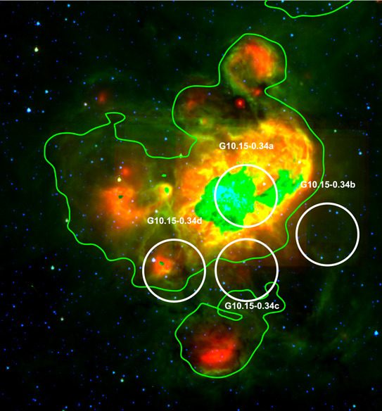
Figure 4. Spitzer three-color images of the UCH ii envelope G10.15-0.34. GLIMPSE 3.6 and 8.0 μm data are shown in blue and green, respectively (Benjamin et al. 2003; Churchwell et al. 2009), and MIPSGAL 24 μm data in red (Carey et al. 2009). The observed positions are indicated in circles of diameter equal to the size of the GBT beam. The image spans the same sky region as shown in Figure 1. Note that near the position G10.14-0.34a the measured flux density at 24 μm is affected owing to detector saturation. The 21 cm radio contour of level 10−2 Jy beam−1 is also shown.
Download figure:
Standard image High-resolution image
Figure 5. Same as Figure 4, except for the UCH ii envelope G23.46-0.20. The image spans the same sky region as shown in Figure 2.
Download figure:
Standard image High-resolution image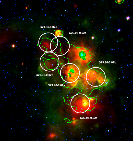
Figure 6. Same as Figure 4, except for the UCH ii envelope G29.96-0.02. The image spans the same sky region as shown in Figure 3. Note that near the position G29.96-0.02a the measured flux density at 24 μm is affected owing to detector saturation.
Download figure:
Standard image High-resolution imageTable 1. Properties of the Selected Sources
| Properties | Value | Reference |
|---|---|---|
| G10.15-0.34 | ||
| Distance | 3.6 kpc | 1 |
| UCH ii regions | G10.15-0.34 | 2 |
| Angular size of envelope | 109 × 67 |
3 |
| Linear size of envelopea | 11.3 pc × 6.9 pc | |
| Flux density of envelope at 1.43 GHz | 55.22 Jy | 3 |
| Assumed electron temperature of the ionized gas | 8000 K | |
| Lyman continuum luminosityb | 6.0 × 1049 s−1 | |
| Star typec | O3 V | |
| G23.46-0.20 | ||
| Distance | 6 kpc | 4, 5 |
| UCH ii regions | G23.455-0.201 | 2 |
| Angular size of envelope | 88 × 58 |
3 |
| Linear size of envelopea | 15.4 pc × 10.1 pc | |
| Flux density of envelope at 1.43 GHz | 11.31 Jy | 3 |
| Assumed electron temperature of the ionized gas | 8000 K | |
| Lyman continuum luminosityb | 3.5 × 1049 s−1 | |
| Star typec | O4.5 V | |
| G29.96-0.02 | ||
| Distance | 6.2 kpc | 6 |
| UCH ii regions | G29.95-0.01, G29.86-0.04 | 2, 6 |
| Angular size of envelope | 63 × 52 |
3 |
| Linear size of envelopea | 11.7 pc × 9.4 pc | |
| Flux density of envelope at 1.43 GHz | 12.69 Jy | 3 |
| Assumed electron temperature of the ionized gas | 8000 K | |
| Lyman continuum luminosityb | 4.2 × 1049 s−1 | |
| Star typec | O4 V | |
Notes.
aLinear size is estimated using the distance give in the table here. bLyman continuum luminosity is estimated as described in Rubin (1968) using the flux density at 1.43 GHz, distance to the source, and electron temperature given in the table here. No correction for dust extinction is applied. cType of the star from the estimated Lyman continuum luminosity using the results of Martins et al. (2005).References. (1) Urquhart et al. 2012; (2) Wood & Churchwell 1989; (3) Kim & Koo 2001; (4) Wienen et al. 2015; (5) Brunthaler et al. 2009; (6) Zhang et al. 2014.
Download table as: ASCIITypeset image
2.1. G10.15-0.34
The G10.15-0.34 region is part of the W31 star-forming complex (Shaver & Goss 1970). Numerous H ii regions and star clusters are present in this well-known star-forming region (Beuther et al. 2011). G10.15-0.34 is one of the dominant infrared and radio continuum sources in W31 and is referred to as W31-South. The UCH ii region G10.15-0.34 is located in the complex W31-South (Wood & Churchwell 1989). The distance to W31 is very uncertain since different indicators provide different distances ranging from near (∼2 kpc) to far (∼15 kpc) kinematic distances (Deharveng et al. 2015). Infrared spectrophotometric analysis of O stars in the H ii region indicates that G10.15-0.34 is at 3.55 kpc (Blum et al. 2001; Moisés et al. 2011). H i absorption studies resolve the kinematic distance ambiguity, indicating a near distance of about 3.55 kpc (Urquhart et al. 2012). Trigonometric parallax measurements provide a distance to the W31 complex of 4.95 kpc (Sanna 2014). The measured parallax is for the H2O maser source in G10.62-00.38, one of the H ii regions in the W31 complex. This H ii region is about 0 5 away from G10.15-0.34, which corresponds to a projected separation on the sky of about 30–40 pc depending on the assumed distance. It is possible that the two H ii regions are at different distances. Here we adopt a distance of 3.55 kpc for the G10.15-0.34 region and for the UCH ii region G10.15-0.34 (see Table 1).
The UCH ii region G10.15-0.34 is located at the western peak in the 21 cm image of the region G10.15-0.34 (see Figure 1). The diffuse gas surrounding the UCH ii region has an angular extent of 109 × 67, which corresponds to a linear size of 11.3 pc × 6.9 pc at the distance of 3.55 kpc. The Lyman continuum photon flux (not corrected for dust extinction) obtained from the 21 cm continuum flux density for the diffuse gas is 3.5 × 1049 s−1, corresponding to a single ionizing star of type O3 V (Martins et al. 2005). We use a temperature for the ionized gas of 8000 K and a flux density at 21 cm of 55.22 Jy (Kim & Koo 2001) to estimate the Lyman continuum photon flux (Rubin 1968). The Lyman continuum photon flux obtained from 21 cm emission is a lower limit of the ionizing luminosity, due to radio continuum optical depth effects and possible escape of UV photons. The diffuse 21 cm emission spatially coincides with a complex ionization ridge seen in the high angular resolution (7 5 × 43) 5 GHz continuum image of G10.15-0.34 (Ghosh et al. 1989). Near-IR (NIR) spectrophotometric study of a 17 × 18 region centered at R.A. 18:09:26.71, decl. −20:19:29.7 (J2000; roughly coincides with the position G10.15-0.34a in Table 2) has identified four O5.5-type stars, which together can account for most of the radio-derived Lyman continuum emission of the UCH ii envelope (Blum et al. 2001).
Table 2. Summary of Observation
| Source | R.A.(2000) | Decl.(2000) | Obs. Time | RRLs Averaged | Eff. Int. |
|---|---|---|---|---|---|
| (minutes) | (hr) | ||||
| G10.15-0.34 | |||||
| G10.15-0.34a | 18:09:23.5 | −20:19:25 | 4.9 | 104, 109, 110, 111, 113 | 0.8 |
| G10.15-0.34b | 18:09:09.5 | −20:21:00 | 14.6 | 104, 109, 110, 111 | 2.0 |
| G10.15-0.34c | 18:09:23.5 | −20:22:25 | 9.8 | 104, 109, 110, 111 | 1.3 |
| G10.15-0.34d | 18:09:36.0 | −20:22:25 | 9.8 | 104, 109, 110, 111 | 1.3 |
| G23.46-0.20 | |||||
| G23.46-0.20a | 18:34:44.7 | −08:32:17 | 7.3 | 104, 109, 110, 111, 113 | 1.2 |
| G23.46-0.20b | 18:34:32.7 | −08:32:17 | 9.8 | 104, 109, 110, 111 | 1.3 |
| G23.46-0.20c | 18:34:24.7 | −08:33:60 | 9.8 | 104, 109, 110, 111 | 1.3 |
| G23.46-0.20d | 18:35:03.7 | −08:33:09 | 9.8 | 104, 109, 110, 111 | 1.3 |
| G23.46-0.20e | 18:35:13.7 | −08:33:08 | 9.8 | 104, 109, 110, 111 | 1.3 |
| G23.46-0.20f | 18:35:40.6 | −08:30:21 | 9.8 | 104, 109, 110, 111 | 1.3 |
| G29.96-0.02 | |||||
| G29.96-0.02a | 18:46:10.4 | −02:41:45 | 4.9 | 104, 109, 110, 111, 113 | 0.8 |
| G29.96-0.02b | 18:45:56.8 | −02:42:16 | 9.8 | 104, 109, 110, 111 | 1.3 |
| G29.96-0.02c | 18:46:15.8 | −02:38:15 | 9.8 | 104, 109, 110, 111 | 1.3 |
| G29.96-0.02d | 18:46:20.8 | −02:40:14 | 9.8 | 104, 109, 110, 111 | 1.3 |
| G29.96-0.02e | 18:46:21.8 | −02:37:44 | 9.8 | 104, 109, 110, 111 | 1.3 |
| G29.96-0.02f | 18:46:04.9 | −02:45:45 | 8.1 | 104, 109, 110, 111 | 1.1 |
Download table as: ASCIITypeset image
2.2. G23.46-0.20
The 21 cm image of the G23.46-0.20 region is shown in Figure 2 (Kim & Koo 2001). The UCH ii region G23.455-0.201 (Wood & Churchwell 1989) is located slightly north of the strongest continuum peak in the 21 cm emission (marked as a star in Figure 2). The LSR velocity of the H76α RRL observed toward the UCH ii region is 99.0 km s−1 (Kim & Koo 2001). Sewilo et al. (2004) analyzed the LSR velocity of the molecular cloud associated with the UCH ii region and placed it at the near-kinematic distance of about 6 kpc (see Wienen et al. 2015). The distance to the 12 GHz methanol source G23.44-0.18 obtained from parallax measurements is 5.88 kpc (Brunthaler et al. 2009). Based on the parallax measurement and LSR velocity study, we adopt a distance to the G23.46-0.20 region of 6 kpc (see Table 1).
The G23.46-0.20 region is located in the direction of the Galaxy where several stellar clusters, supernova remnants (SNRs), and giant molecular clouds are present (Messineo et al. 2014). The diffuse gas surrounding the UCH ii region exhibits two peaks in the 21 cm continuum emission separated in the north–south direction (see Figure 2). The strongest peak (marked as a triangle in Figure 2) coincides with the IR source G23.437-0.209 (Conti & Crowther 2003). The 21 cm continuum emission is elongated in the east–west direction, part of which coincides with the shell of the W41 SNR (Leahy & Tian 2008). The angular size of the G23.46-0.20 region is 88 × 58. At the distance of 6 kpc, the linear size of the diffuse emission region is 15.4 pc × 10.1 pc. The Lyman continuum luminosity (not corrected for dust extinction and contamination from W41 SNR emission) obtained from the integrated radio flux density at 21 cm (11.31 Jy; Kim & Koo 2001) is 4.0 × 1049 s−1, for an assumed ionized gas temperature of 8000 K. If a single star is responsible for the ionizing luminosity, then the type of the star is O4.5 V (Martins et al. 2005).
2.3. G29.96-0.02
G29.96-0.02 is a well-known star-forming region in the inner Galaxy. It is part of the W43 complex and is referred to as W43-South. The 21 cm continuum image of the region is shown in Figure 3 (Kim & Koo 2001). The location of the cometary UCH ii region G29.95-0.01 (Wood & Churchwell 1989) coincides with the strongest continuum peak (see Figure 3). Trigonometric parallax measurements were made toward two 12 GHz methanol sources in the G29.96-0.02 region—one associated with the UCH ii region G29.95-0.01, and the second toward G29.86-0.04. The distances obtained to the two sources are 6.21 and 5.26 kpc, respectively (Zhang et al. 2014). Here we adopt 6.2 kpc as the distance to the G29.96-0.02 region (see Table 1).
The 21 cm emission from G29.96-0.02 is extended over 63 × 52, corresponding to a linear size of 11.7 pc × 9.4 pc. The NRAO/VLA Sky Survey (NVSS), which has an angular resolution of 45'', has cataloged 10 sources consisting of both unresolved and extended objects (Condon et al. 1998). The brightest NVSS source is associated with the cometary UCH ii region G29.95-0.01 (Wood & Churchwell 1989). The physical properties of the NVSS sources were obtained from their radio continuum emission (Beltrán et al. 2013). These sources harbor stars of type O5–B0. The giant H ii region G29.944-0.042 is located southeast of G29.95-0.01. The Lyman continuum photon flux estimated using the flux density at 21 cm (12.69 Jy; Kim & Koo 2001) is 4.8 × 1049 s−1. The temperature of the ionized gas is assumed to be 8000 K for estimating the Lyman continuum luminosity, and no dust extinction correction is applied. The luminosity can be produced by a single ionizing star of type O4 V (Martins et al. 2005). K-band spectroscopy shows that the central exciting star of the UCH ii region G29.95-0.01 is of type O5 (Hanson et al. 2005). Note that the estimated Lyman continuum luminosity is only 44% of that obtained for the giant H ii region G29.944-0.042 from 6 cm continuum observations (Conti & Crowther 2004). The 6 cm source size obtained for G29.944-0.042 is 37 (Kuchar & Clark 1997). We attribute this discrepancy to radio continuum optical depth effects at 21 cm.
3. Observation and Data Reduction
The sizes of the selected sources are listed in Table 1. The typical physical size of the selected diffuse regions surrounding UCH ii regions is ≳9 pc, which corresponds to an angular size ≳5'. We made RRL observations toward 13 positions in the selected sources with the Robert C. Byrd Green Bank Telescope (GBT) near 5 GHz. The FWHM beam width of the telescope near 5 GHz was about 25, allowing us to sample physical scales smaller than the sizes of the diffuse regions in the selected sources. The J2000 R.A. and decl. of the observed positions are listed in Table 2 and are shown in Figures 1–3. For comparison, we also observed three positions (G10.15-0.34a, G23.46-0.20a, G29.96-0.02a; see Figures 1–3 and Table 2) toward peaks in the 21 cm continuum images of the selected regions.
We simultaneously observed eight RRL transitions (104α, 105α, 106α, 109α, 110α, 111α, 112α, and 113α) of hydrogen, helium, and heavy elements. The reference spectra to correct for bandpass shape were obtained by switching the frequency by 8.5 MHz (∼530 km s−1). GBTIDL routines were used to correct for bandpass shape for each RRL transition and calibrate the spectra in units of antenna temperature. Doppler tracking was done using the H110α RRL transition during observation. The residual Doppler correction in other RRL transitions was done offline by shifting them in LSR velocity. The Doppler-corrected spectra for each RRL transition were averaged using GBTIDL routines. The rest of the data analysis was done using routines developed in Matlab. The average spectrum for each transition was examined for radio frequency interference (RFI). After editing RFI-affected spectra and removing spectra that have beta transitions contaminating the helium line, we resampled the subset of RRL spectra to a common velocity resolution. This subset was averaged to obtain the final integrated spectrum. The RRL transitions averaged to get the final spectrum are listed in Table 2. The actual observing time and effective integration time, obtained from the number of transitions averaged, for each position are also included in Table 2. The effective integration time is the actual integration time of the final spectra after editing out the RFI-affected spectra and averaging the data corresponding to the listed transitions in Table 2. A fourth-order polynomial was subtracted from the final spectrum.
4. Results
Results of Gaussian component analysis of the final spectra are included in Table 3. The source name, peak line antenna temperature in K, FWHM line width in km s−1, LSR velocity of the line in km s−1, and the atom responsible for the line emission are included in Table 3. The final spectra and the Gaussian components are shown in Figures 1–3. The signal-to-noise ratio of the hydrogen line is greater that 10σ in most cases, allowing us to fit multiple Gaussian components to the line profile. We choose the minimum number of Gaussian components for the hydrogen line so that the residuals after subtracting the Gaussian model are consistent with the rms of the spectral noise. Since we did not know a priori which hydrogen line component corresponds to the helium line, we tried several methods to obtain the helium line parameters. We found that the different methods provide a slightly different value for the  ratio (see below), but all these values are consistent within the 1.5σ estimation error of this ratio. We finally adopted the following strategy to get the helium line parameters: we set the LSR velocity of the helium line equal to the central velocity of the strongest hydrogen line while fitting the Gaussian components. The exception is for the position G10.15-0.34d, where the helium line velocity is close to the 8.45 km s−1 hydrogen line component, and hence we used this velocity for the central velocity of helium. No constraints were used to obtain line parameters of atoms heavier than helium. The heavy element is tentatively identified as carbon based on its frequency and its relatively high abundance compared to other heavy elements with ionization potential <13.6 eV.
Table 3. Observed Line Parameters
| Source | TLa | ΔVa | VLSRa | Line |
|---|---|---|---|---|
| (K) | (km s−1) | (km s−1) | ||
| G10.15-0.34a | 2.071 (0.034) | 27.38 (0.2) | 13.03 (0.03) | H |
| 0.972 (0.035) | 51.68 (0.6) | 13.17 (0.09) | H | |
| 0.116 (0.018) | 27.42 (1.1) | 13.03 (0.00) | He | |
| 0.056 (0.005) | 34.46 (6.3) | 21.33 (3.86) | Cb | |
| G10.15-0.34b | 0.047 (0.001) | 36.98 (0.4) | 16.13 (0.18) | H |
| ≤0.002 | He, C | |||
| G10.15-0.34c | 0.048 (0.004) | 24.47 (1.3) | 12.77 (0.34) | H |
| 0.071 (0.005) | 48.06 (1.0) | 6.29 (0.46) | H | |
| ≤0.003 | He, C | |||
| G10.15-0.34d | 0.067 (0.003) | 19.15 (0.6) | 8.46 (0.18) | H |
| 0.092 (0.003) | 43.56 (0.5) | 16.34 (0.30) | H | |
| 0.006 (0.001) | 14.86 (2.7) | 8.46 (0.00) | He | |
| ≤0.003 | C | |||
| G10.15-0.34avgc | 0.064 (0.001) | 38.98 (0.3) | 12.83 (0.13) | H |
| ≤0.002 | He,C | |||
| G23.46-0.20a | 0.547 (0.001) | 24.08 (0.1) | 101.06 (0.04) | H |
| 0.040 (0.001) | 30.26 (1.4) | 64.60 (0.58) | H | |
| 0.033 (0.001) | 19.41 (1.1) | 101.06 (0.00) | He | |
| 0.015 (0.002) | 9.50 (1.6) | 102.50 (0.68) | C | |
| G23.46-0.20b | 0.289 (0.001) | 22.75 (0.1) | 99.10 (0.06) | H |
| 0.025 (0.001) | 22.95 (1.6) | 57.32 (0.65) | H | |
| 0.013 (0.001) | 15.38 (2.0) | 99.10 (0.00) | He | |
| 0.009 (0.002) | 7.34 (2.0) | 102.10 (0.87) | C | |
| G23.46-0.20c | 0.233 (0.001) | 19.48 (0.1) | 98.10 (0.05) | H |
| 0.022 (0.001) | 27.87 (1.7) | 58.17 (0.67) | H | |
| 0.013 (0.001) | 12.44 (1.4) | 98.10 (0.00) | He | |
| ≤0.003 | C | |||
| G23.46-0.20d | 0.040 (0.001) | 15.30 (0.7) | 57.03 (0.36) | H |
| 0.026 (0.001) | 23.97 (1.7) | 99.94 (0.86) | H | |
| 0.016 (0.001) | 17.54 (3.3) | 76.78 (0.97) | H | |
| ≤0.002 | He, C | |||
| G23.46-0.20e | 0.045 (0.001) | 16.87 (0.7) | 59.15 (0.32) | H |
| 0.035 (0.001) | 26.24 (1.7) | 95.61 (1.00) | H | |
| 0.021 (0.003) | 14.17 (2.0) | 77.70 (0.66) | H | |
| ≤0.003 | He, C | |||
| G23.46-0.20f | 0.049 (0.001) | 26.47 (0.5) | 89.20 (0.19) | H |
| 0.014 (0.001) | 17.82 (1.3) | 57.34 (0.55) | H | |
| ≤0.002 | He, C | |||
| G23.46-0.20avgd | 0.026 (0.001) | 15.89 (0.5) | 56.87 (0.21) | H |
| 0.035 (0.001) | 32.32 (0.6) | 90.36 (0.22) | H | |
| ≤0.002 | He, C | |||
| G29.96-0.02a | 0.512 (0.016) | 29.11 (0.4) | 101.35 (0.11) | H |
| 0.083 (0.014) | 46.37 (1.5) | 89.35 (2.21) | H | |
| 0.045 (0.002) | 26.94 (1.1) | 101.35 (0.00) | He | |
| 0.018 (0.004) | 4.97 (1.1) | 99.67 (0.48) | C | |
| G29.96-0.02b | 0.461 (0.005) | 19.85 (0.1) | 99.28 (0.04) | H |
| 0.054 (0.005) | 40.26 (1.3) | 93.58 (0.62) | H | |
| 0.033 (0.001) | 19.18 (0.7) | 99.28 (0.00) | He | |
| 0.014 (0.001) | 10.11 (1.2) | 97.09 (0.51) | C | |
| G29.96-0.02c | 0.180 (0.005) | 18.23 (0.3) | 95.45 (0.07) | H |
| 0.035 (0.005) | 43.33 (2.6) | 95.25 (0.56) | H | |
| 0.013 (0.001) | 13.55 (1.6) | 95.45 (0.00) | He | |
| ≤0.003 | C | |||
| G29.96-0.02d | 0.141 (0.003) | 19.11 (0.3) | 96.02 (0.07) | H |
| 0.040 (0.003) | 46.11 (1.7) | 95.91 (0.38) | H | |
| 0.010 (0.001) | 15.94 (1.6) | 96.02 (0.00) | He | |
| ≤0.003 | C | |||
| G29.96-0.02e | 0.166 (0.002) | 20.07 (0.2) | 96.89 (0.07) | H |
| 0.014 (0.002) | 56.08 (3.7) | 87.29 (1.85) | H | |
| 0.012 (0.001) | 15.57 (1.5) | 96.89 (0.00) | He | |
| ≤0.003 | C | |||
| G29.96-0.02f | 0.283 (0.002) | 19.67 (0.2) | 97.68 (0.07) | H |
| 0.023 (0.002) | 14.50 (1.4) | 97.68 (0.00) | He | |
| 0.007 (0.003) | 8.25 (3.5) | 102.62 (1.47) | C |
Notes.
a1σ errors in the estimated quantities are given in parentheses. The upper limits on line temperature are 1σ limits. If a parameter is fixed during Gaussian fitting, then the corresponding error is set to 0.0. bThis line component is tentatively identified as due to carbon atoms based on its LSR velocity offset from the hydrogen RRL. However, we note the larger line width compared to the typical width (≲10 km s−1) of carbon lines observed toward PDRs. cSpectrum obtained by averaging the data toward positions G10.15-0.34b and G10.15-0.34c. dSpectrum obtained by averaging the data toward positions G23.46-0.20d and G23.46-0.20f.4.1. LSR Velocity of Hydrogen Line
The LSR velocity structure of the hydrogen lines toward the observed sources was studied earlier by Kim & Koo (2001). We reexamine the line velocity structure with our new, sensitive RRL observations. The line structure in general is complex, exhibiting multiple velocity components toward all three sources. Toward the four observed positions in G10.15-034, the peak hydrogen line velocity ranges between 16.3 and 6.3 km s−1, with a mean value of 12.3 km s−1. The velocity spread of this source is attributed to bipolar flow exhibited by the ionized gas (Kim & Koo 2001). A bipolar flow is also inferred from the velocity structure of dense molecular tracers observed toward G10.15-034 (Kim & Koo 2003; Deharveng et al. 2015). The mean velocity of the molecular tracers is in good agreement with that of the RRLs. Thus, the diffuse gas observed toward G10.15-034 is likely to be associated with the UCH ii region G10.15-034 as concluded earlier by Kim & Koo (2001). The size of the diffuse region is about 8 pc (see Table 1), much larger than the UCH ii region, and hence multiple massive stars in the star-forming region will be contributing to the ionization of the diffuse gas.
The hydrogen line toward G23.46-0.20 shows at least three LSR velocity components, ∼60, 76, and 95 km s−1. The LSR velocity of the hydrogen line observed toward the UCH ii region is 99 km s−1 (Kim & Koo 2001), and hence it is likely that only the 95 km s−1 component is associated with the source G23.46-0.20. This is because there is no evidence for outflows with such large velocity difference to produce the other line components. Further, the kinematic distances of the 60 and 76 km s−1 line components are greater than 1 kpc from that of the 95 km s−1 component. Thus, the 60 and 76 km s−1 components are most likely due to ionized gas along the line of sight. The 95 km s−1 component in our data shows a velocity range from 89.2 to 101.1 km s−1 over the six observed positions toward the source, with a mean value of 97.2 km s−1. The 13CO line observed toward G23.46-0.20 shows a similar velocity range. The velocity structures of molecular lines and RRLs have been interpreted as due to a champagne flow (Kim & Koo 2003) and not due to multiple ionized gas locations along the line of sight. As in the case of G10.15-034, the large size of the diffuse gas (12 pc; see Table 1) implies that multiple stars present in the star-forming region G23.46-0.20 may be contributing to the ionization of the diffuse region.
The LSR velocity range of the hydrogen line observed toward six positions in G29.96-0.02 is between 87.3 and 101.4 km s−1, with a mean value of 95.9 km s−1. The mean velocity is similar to the LSR velocity of RRLs (95.3 km s−1) observed toward the UCH ii region (Wood & Churchwell 1989). Molecular line observations show a velocity gradient from ∼92 to 100 km s−1, roughly in agreement with that observed in RRLs. There are several compact H ii regions embedded in the diffuse ionized gas. Thus, the velocity structure of the diffuse gas is likely to be reflecting the blending of ionized gas from the different compact sources.
To summarize, in all three observed sources, we could identify a line component that has LSR velocity similar to that of the UCH ii regions. We consider that this line component is due to emission from the diffuse ionized gas surrounding the UCH ii regions. In the following sections, we refer to the gas with the identified velocity component as the UCH ii envelope. It is likely that several ionizing sources embedded in the diffuse gas are contributing to the ionization of this gas.
4.2. Helium-to-hydrogen Line Ratio
The ratio
obtained from the RRL data is given in Table 4. Here  and
and  are the line antenna temperatures of helium and hydrogen, respectively (see Table 3), and the integration is over LSR velocity. The computed values of the
  ratio, along with 1σ error and upper limits, are listed in column (2) in Table 4. The velocities of the hydrogen line components used to obtain the ratio are given in column (3). In cases where the helium line is not detected, the upper limit for the ratio is computed using the 1σ value at the line-free region of the spectrum and the net line width of the hydrogen line components listed in column (3) as the expected width of the helium line. The other columns are source name (column (1)), offset distance from the "ionization center" (column (4); see below), 4.875 GHz brightness temperature (column (5); see below) and emission measure (column (6)). The emission measures are obtained from the main beam brightness temperature, estimated from the 4.875 GHz continuum survey of Altenhoff et al. (1979), which has similar angular resolution to that of the GBT observations. The emission measure is obtained using the equation (Mezger & Henderson 1967)

where EM has units pc cm−6,  is the brightness temperature in K at the frequency ν = 4.875 GHz, and Te is the electron temperature in K (see Table 1).
Table 4.
 Ratio toward the Observed Positions
| Source |
 a
a
|
VLSR | Offset |
 b
b
|
EM |
|---|---|---|---|---|---|
| (km s−1) | (pc) | (K) | (pc cm−6) | ||
| G10.15-0.34a | 0.056 (0.009) | 13.03 | 0.9 | 50.0 | 4.0 × 10⁵ |
| G10.15-0.34b | ≤0.052 | 16.13 | 4.7 | 5.0 | 4.0 × 10⁴ |
| G10.15-0.34c | ≤0.037 | 12.77, 6.29 | 3.1 | 5.0 | 4.0 × 10⁴ |
| G10.15-0.34d | 0.073 (0.018) | 8.46 | 3.9 | 5.0 | 4.0 × 10⁴ |
| G10.15-0.34avg | ≤0.033 | 12.83 | 3.9 | ⋯ | 4.0 × 10⁴ |
| G23.46-0.20a | 0.048 (0.003) | 101.06 | 2.0 | 8.0 | 6.4 × 10⁴ |
| G23.46-0.20b | 0.031 (0.005) | 99.10 | 5.7 | 6.0 | 4.8 × 10⁴ |
| G23.46-0.20c | 0.035 (0.005) | 98.10 | 10.1 | 3.6 | 2.9 × 10⁴ |
| G23.46-0.20d | ≤0.094 | 99.94 | 9.0 | 2.0 | 1.6 × 10⁴ |
| G23.46-0.20e | ≤0.072 | 95.61 | 13.0 | 1.8 | 1.4 × 10⁴ |
| G23.46-0.20f | ≤0.050 | 89.20 | 24.4 | 1.1 | 8.7 × 10³ |
| G23.46-0.20avg | ≤0.051 | 90.36 | 15.5 | ⋯ | 1.2 × 10⁴ |
| G29.96-0.02a | 0.081 (0.005) | 101.35 | 5.2 | 10.0 | 7.9 × 10⁴ |
| G29.96-0.02b | 0.069 (0.003) | 99.28 | 6.1 | 8.0 | 6.4 × 10⁴ |
| G29.96-0.02c | 0.053 (0.008) | 95.45 | 5.7 | 4.0 | 3.2 × 10⁴ |
| G29.96-0.02d | 0.061 (0.008) | 96.02 | 7.8 | 2.8 | 2.2 × 10⁴ |
| G29.96-0.02e | 0.058 (0.007) | 96.90 | 8.6 | 2.4 | 1.9 × 10⁴ |
| G29.96-0.02f | 0.061 (0.008) | 97.68 | 11.5 | 3.0 | 2.4 × 10⁴ |
Notes.
a1σ error in the estimated quantity is given in parentheses. The upper limits are also the 1σ limit. bMain-beam brightness temperature at 4.875 GHz at the observed positions obtained from the galactic plane survey of Altenhoff et al. (1979).Download table as: ASCIITypeset image
The helium lines are detected toward G10.15-0.34a and d in G10.15-0.34. We use the 24 μm emission in the MIPSGAL data, which has higher angular resolution (∼6'') than the 21 cm images, to identify compact H ii regions (emission shown in red in Figure 4) in the observed positions. This identification can be done because a large part of the 24 μm emission originates from very small dust grains (few nanometers in size) inside H ii regions heated by UV radiation from the star and collision with ionized gas particles (Pavlyuchenkov et al. 2013). The observed correlation between the 24 μm emission and 21 cm flux density of Galactic H ii regions supports this picture (Anderson et al. 2014). Both these positions have bright 24 μm emission, indicating the presence of compact H ii regions. Helium lines are not detected toward G10.15-0.34c and b. No compact H ii regions are present in these directions as inferred from the 24 μm image. We averaged the GBT spectra observed toward these two positions to get a stringent upper limit on helium line emission. The line parameters obtained from the average spectrum are listed in Table 3. The LSR velocity of the hydrogen line (12.8 km s−1) is similar to those observed toward other positions in the source G10.15-0.34. Thus, the positions G10.15-0.34c and b sample the more diffuse region of the UCH ii envelope. The 1σ upper limit for helium line emission and the value of the  toward the diffuse region are ∼2 mK and 0.03, respectively, both obtained from the average spectrum shown in Figure 7.
Helium lines are detected toward positions G23.46-0.20a, b, and c. Examination of the 24 μm image indicates that compact H ii regions are present in these regions (see Figure 5). No helium lines were detected toward positions G23.46-0.20d, e, and f. Toward the position G23.46-0.20e a compact H ii region is present, as inferred from its 24 μm emission. The hydrogen lines toward positions G23.46-0.20d and f have components with LSR velocities 99.9 and 89.2 km s−1, respectively. The strongest hydrogen line components toward positions G23.46-0.20a, b, c, and e show a gradient in LSR velocity with values reducing from 101.1 to 95.6 km s−1. Thus, the diffuse ionized gas toward G23.46-0.20d and G23.46-0.20f may be associated with G23.46-0.20. We averaged the GBT spectra toward G23.46-0.20d and f to get a stringent upper limit on helium line emission (see Figure 7). The upper limit for the value of the  obtained from this average spectrum is 0.05.
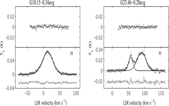
Figure 7. Spectra obtained by averaging the data from positions G10.15-0.34b and G10.15-0.34c (left) and from positions G23.46-0.20d and G23.46-0.20f (right). The observed spectra (indicated by crosses), the Gaussian line components (solid line), and the residual spectra (dotted line) for hydrogen lines are shown in the bottom panels. The helium spectra are shown in the top panels.
Download figure:
Standard image High-resolution imageHelium lines are detected toward all the observed positions in G29.96-0.02. All these positions have associated bright 24 μm emission, indicating the presence of compact H ii regions (see Figure 6). The value of  varies between 0.053 and 0.081 at the observed positions. Such variation is also observed toward the sources G10.15-0.34 and G23.46-0.20 at positions where helium lines are detected.
Figure 8 shows the histogram of the values for  obtained toward positions where helium lines are detected from all three sources. The values of the ratio from our sample range from 0.033 to 0.081; the mean value is 0.058. The mean value for
  is consistent with those observed toward compact H ii regions in the Galaxy (Churchwell et al. 1974; Quireza et al. 2006). It may be noted that some of the H ii regions observed by Churchwell et al. (1974) and Quireza et al. (2006) may be ionized by stars later than O6, and hence the mean value of
  from their data set is biased toward lower values.

Figure 8. Histogram of the observed  ratio.
Download figure:
Standard image High-resolution imageMultiple OB stars are responsible for the ionization of the observed sources. Due to the complexity of the source, however, it is difficult to identify a region, referred to as the "ionization center," where most of the massive stars are located in each source. We assigned the "ionization center" for the region G10.15-0.34 as the center of the NIR emission observed by Blum et al. (2001) (R.A. 18:09:26.71, decl. −20:19:29.7 J2000; see Section 2; shown in Figure 1), which has revealed four O-type stars. The "ionization center" for the region G23.46-0.20 is taken as the UCH ii region G23.455-0.201, and that for the region G29.96-0.02 is taken as the UCH ii region G29.95-0.01. In Figure 9, we plot the values of the  ratio against the estimated distance offset (see Table 4) of the observed positions from the "ionization center." We also plot the measured
  values against the estimated emission measure (see Table 4) in Figure 10. The upper limits obtained from the average spectra are shown in the plot with filled triangles. No particular trends are evident in these plots, but it is clear that the helium is not uniformly ionized in the observed regions.
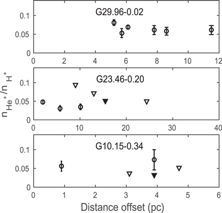
Figure 9. Observed  ratio with ±1.5σ error bar vs. distance from the "ionization center" (see text). The 1σ upper limits on the ratio from nondetections are indicated by open triangles. The filled triangles are 1σ upper limits obtained from the average spectra.
Download figure:
Standard image High-resolution image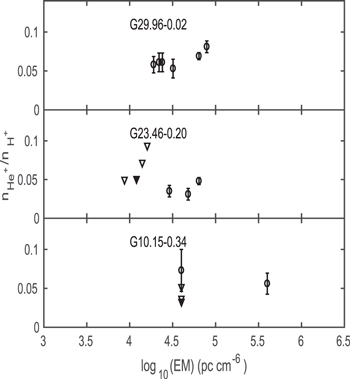
Figure 10. Observed  ratio with ±1.5σ error bar vs. emission measure. The 1σ upper limits on the ratio from nondetections are indicated by open triangles. The filled triangles are 1σ upper limits obtained from the average spectra.
Download figure:
Standard image High-resolution image5. Discussion
We first examine the observed  ratio toward the continuum bright regions (G10.15-0.34a, G23.46-0.20a, and G29.96-0.02a). The first two positions encompass the UCH ii regions G10.15-0.34 and G23.455-0.201, respectively. The third position is observed near the giant H ii region G29.944-0.042. The mean value of the
  ratio obtained from the data toward the three positions is 0.062 ± 0.02. This value is slightly lower than the mean value of
  (0.08 ± 0.02) observed toward H ii regions ionized by stars of spectral type O6 or hotter star (Shaver et al. 1983). The origin of this lower
  value may be related to the nonuniform helium ionization observed in the selected sources.
In the diffuse regions in the sources G10.15-0.34 and G23.46-0.20 less than 33% and 51%, respectively, of the helium is singly ionized. The detection of helium lines toward high emission measure regions in the envelopes implies that stars of type O6 or earlier are embedded in these regions. If these stars are responsible for the ionization of the diffuse gas, then helium is expected to be fully ionized. Thus, the situation in the UCH ii envelopes is similar to the WIM and DIR—i.e., stars of type O6 or earlier are required for the ionization of the WIM and DIR, but helium in these regions is observed to be not fully ionized. Observations toward the WIM and DIR probe helium ionization at distances greater than a few tens of parsec from the ionizing stars. Our observations, on the other hand, probe helium ionization in diffuse regions at distances ≲10 pc from newly born massive stars. Below we investigate possible origins for the nonuniform helium ionization.
As mentioned earlier, stars hotter than ∼O6 are the likely primary ionization sources of the DIR and WIM. A "hardening" of the radiation field with distance from the ionizing source is expected since the the ionization cross sections for both H and He decrease with energy proportional to (hν)−3. If that is the case, can helium be doubly ionized in regions where He+ lines are not detected? The velocity range of RRL spectra obtained in our observation includes 167α, 175α, and 178α recombination line transitions of He++. The velocity range of 167α transition overlaps with the H105α line. The 178α transition is affected by a bad baseline. We therefore examined the 175α transition of He++ but failed to detect the line from any of the observed positions. We further averaged the spectra from all the observed positions after resampling and shifting them in velocity, but again failed to detect the He++ line. The 1σ upper limit we obtained is 0.004 K. Thus, we conclude that helium is not doubly ionized at the observed positions.
The sizes of the helium and hydrogen ionization zones depend on the number of "helium" (qHe; i.e., photon wavelength range 228 Å < λ < 504 Å) and "hydrogen" (qH; i.e., photon wavelength range 504 Å < λ < 912 Å) Lyman photons available for ionization (Mathis 1971). It is convenient to characterize the Lyman photon spectrum by the ratio  (Mathis 1971). To understand physically the dependence of the ionization zone size on γ, to a first approximation, we assume (a) that all the qHe photons ionize helium and (b) that the photons due to the recombination of helium ions ionize hydrogen. The first assumption is justified since the ionization cross section of helium for energies ≥24.6 eV is larger compared to that of hydrogen. The second assumption follows from the energy level of helium and the probability of the paths involved in the recombination process. With the above assumptions and keeping in mind that the helium recombination rate is ∼18% of that of hydrogen in regions where both atoms are (singly) ionized, the ionization equilibrium implies that the size of the helium ionization zone is smaller than the hydrogen ionization zone if γ ≲ 0.2 (see Draine 2011, p. 172, for further reading). A numerical solution to this problem was presented by Mathis (1971), where he derived the relationship between γ and the sizes of the ionization zones of the two atoms (see Appendix
  ratio?
In Appendix  ratios are used to obtain γ for the radiation field as described in Appendix
  for G10.15-0.34 and G23.46-0.2 are ∼0.03 and 0.05, respectively. The estimated γ for the two sources are, respectively, 0.04 and 0.06. Thus, from Figure 11, it follows that the upper mass of the cluster member that ionizes these UCH ii envelopes has to be ≲30 M⊙ to explain the observed value of the
  ratio. The Lyman continuum emission estimated for G10.15-0.34 and G23.46-0.2 is ∼5 × 1049 s−1 (average value for these two sources from Table 1). If all the cluster members are contributing to the ionization, then the mean ionizing flux per solar mass is 6.1 × 1046 s−1 M⊙−1 (see Appendix
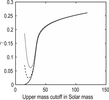
Figure 11. Helium-to-hydrogen Lyman photon ratio, γ, vs. upper cutoff mass of the cluster. The continuous curve shows γ for ionizing radiation due to OB stars alone. A modified version of the Muench IMF is considered for the computation (see Appendix
Download figure:
Standard image High-resolution imageThe infrared (IR) continuum emission from H ii regions is reprocessed stellar radiation from dust. The bolometric luminosity of H ii regions estimated from the IR emission can thus be used to infer the stellar type. For several H ii regions, the estimated Lyman continuum luminosities, obtained from their radio free–free emission, exceed those expected from their inferred stellar type (Wood & Churchwell 1989; Sánchez-Monge et al. 2013). It has been suggested that this excess ionizing radiation is due to accreting low-mass stars present in the star-forming region (Smith 2014). The "hot" spots on the stellar surface in such accreting stars form the additional source for Lyman continuum emission. We investigate whether the presence of such accreting low-mass stars in our observed sources can contribute to the hydrogen Lyman photons, thus modifying the net γ. The details of the analysis are given in Appendix  ratio observed toward the selected sources.
Finally, we investigate whether selective absorption of Lyman photons due to dust in the H ii regions can produce the observed low  ratio, as suggested earlier by Mezger et al. (1974). Appendix
  ratio. To estimate the change in γ, we first express the dust absorption cross sections in terms of the extinction cross section at 13.6 eV provided by the Weingartner & Draine (2001) dust model. The ratio of the helium to hydrogen Lyman photon absorption cross sections, a0, is then estimated using the observed
  ratio and taking the γ due to the stellar cluster to be 0.2 (see Appendix
  ratio.
Table 5. Selective Absorption due to Dust
| Properties | Value | Note |
|---|---|---|
| G10.15-0.34 | ||
| Path length (pc) | 4.4 | a |
| Electron density (cm−3) | 135 | b |

|
≤0.033 | From Table 4 |
| γ' | 0.04c | |
| a0 | 4.4 | ϕ = 0.25d, fuv = 0.5d |
| 2.4 | ϕ = 0.64, fuv = 1.0 | |
| 2.9 | ϕ = 0.25, fuv = 1.0 | |
| 2.2 | ϕ = 0.25, fuv = 2.0 | |
| G23.46-0.20 | ||
| Path length (pc) | 6.2 | a |
| Electron density (cm−3) | 62 | b |

|
≤0.051 | From Table 4 |
| γ' | 0.06c | |
| a0 | 4.0 | ϕ = 0.25, fuv = 0.5 |
| 2.1 | ϕ = 0.64, fuv = 1.0 | |
| 2.7 | ϕ = 0.25, fuv = 1.0 | |
| 2.0 | ϕ = 0.25, fuv = 2.0 | |
| G29.96-0.02 | ||
| Path length (pc) | 5.2 | a |
| Electron density (cm−3) | 90 | b |

|
0.053e | From Table 4 |
| γ' | 0.06c | |
| a0 | 3.4 | ϕ = 0.25, fuv = 0.5 |
| 1.9 | ϕ = 0.64, fuv = 1.0 | |
| 2.3 | ϕ = 0.25, fuv = 1.0 | |
| 1.8 | ϕ = 0.25, fuv = 2.0 | |
Notes.
aPath length, , in Equation (11) estimated from the angular size and distance given in Table 1 and assuming a spherical distribution for the ionized gas (Panagia & Walmsley 1978).
bElectron density, ne, in Equation (11) estimated using the Lyman continuum luminosities given in Table 1 and
, in Equation (11) estimated from the angular size and distance given in Table 1 and assuming a spherical distribution for the ionized gas (Panagia & Walmsley 1978).
bElectron density, ne, in Equation (11) estimated using the Lyman continuum luminosities given in Table 1 and  cγ' is obtained from the listed
  ratio as discussed in Appendix
  ratio observed toward G29.96-0.02.
Download table as: ASCIITypeset image
6. Summary
We observed helium and hydrogen RRLs near 5 GHz toward envelopes of three UCH ii regions—G10.15-0.34, G23.46-0.20, and G29.96-0.02. This data set is used to investigate helium ionization in the UCH ii envelopes. Our main results are as follows:
- 1.Our observations indicated that helium was not uniformly ionized in the UCH ii envelopes. Toward G10.15-0.34 and G23.46-0.20 helium lines were not detected in a few positions, and the upper limits obtained for the
 ratio were 0.033 and 0.051, respectively. Our data thus show that helium is not fully ionized in the diffuse regions located at a few parsec from the young massive stars embedded in the observed sources.
 - 2.The mean value of the ratio obtained from the positions nearer to the peak of the radio continuum emission in the observed sources was 0.06 ± 0.02, consistent with the value measured toward compact H ii regions in the Galaxy.
- 3.No He++ RRLs were detected toward the observed sources (1σ upper limit is 4 mK), which ruled out the possibility that helium may be doubly ionized in the diffuse regions of the UCH ii envelopes.
- 4.Toward G10.15-0.34 and G23.46-0.20, we investigated the spectrum of the radiation that ionizes the diffuse regions. We considered that the stars of type O6 and earlier were embedded in (locally) ionization-bounded regions and were not contributing to the ionization of the diffuse regions. The observed upper limit on the ratio then provided an upper mass of ∼30 M⊙ for the cluster members that ionize the diffuse regions. This upper mass, however, is somewhat uncertain owing to statistical uncertainty in the cluster population.
- 5.
- 6.We also investigated whether selective absorption of Lyman photons by dust was responsible for low helium ionization. We found that the ratio of helium and hydrogen absorption cross section of Lyman photons by dust, a0, should be in the range of 1.8–4.4 to account for the observed ratio. However, a self-consistent model for dust absorption cross section over a wide wavelength range needs to be developed to conclusively establish the role of selective absorption.


We thank Drs. Kim and Koo for providing their 21 cm images. We acknowledge the critical comments by an anonymous referee that have significantly improved the presentation of the results in the paper.
Facility: Green Bank Telescope - .
Appendix: Computation of γ and a0
Here we summarize the computation of (a) γ, the helium-to-hydrogen photon number ratio, due to a star cluster; (b) γ with emission from low-mass accreting stars in the cluster; and (c) the parameter a0, which characterizes the selective dust absorption of Lyman photons.
A.1. Expected Helium Ionization due to a Cluster
Computation of hydrogen (qH) and helium (qHe) Lyman photons from a cluster requires a knowledge of these photon emissions by stars of different mass and the mass function of the cluster. We consider here a modified version of the Muench initial mass function (IMF; Muench et al. 2002) discussed by Murray & Rahman (2010):
We used Γ = 1.35, the slope of the Salpeter IMF, for high-mass stars (Murray & Rahman 2010), ml = 0.1 M⊙, m1 = 0.6 M⊙ (m2 = 0.025 M⊙, which is below ml). The maximum value for the upper mass cutoff, mu, is taken as 120 M⊙. N0 is fixed through the normalization

The Lyman photon emission from stars is taken from the models of Martins et al. (2005). With the above IMF and mu = 120 M⊙, we get a mean mass of  M⊙ and mean Lyman continuum photons per s per M⊙
  s−1 M⊙−1. These values are consistent with those obtained by Murray & Rahman (2010). The helium-to-hydrogen Lyman photon number ratio is

where  and
and  are the IMF-weighted helium and hydrogen Lyman photon emission per second. In Equation (7),
  is approximately taken as the Lyman continuum photons with λ < 504 Å (Martins et al. 2005). γ is computed for different mu in the range 15–120 M⊙. The result of the computation is plotted in Figure 11.
A.2. The Effect of Accreting Low-mass Stars
Several H ii regions have Lyman continuum emission in excess of what is expected from the star type determined from their IR emission (Wood & Churchwell 1989; Sánchez-Monge et al. 2013). A model that can account for the excess Lyman photon emission in terms of accreting low-mass stars is presented by Smith (2014) (see also Hosokawa et al. 2010). Recent observation of infall tracers toward Lyman excess H ii regions supports the accretion model (Cesaroni et al. 2016). Here we use Figures 2 and 3 of Smith (2014), which gives respectively the stellar radius and accretion luminosity as a function of the mass of the accreting star. We consider the "cold" accretion case as suggested by Smith (2014). The mass–radius and mass–luminosity relationships are given for different accretion rates. To account for the observed Lyman excess in H ii regions, accretion rates in the range of 10−5 to 10−3 M⊙ yr−1 are required. Calculations here are presented with an accretion rate of 10−4 M⊙ yr−1. The excess Lyman emission originates at "hot" spots created on the surface of the star during "cold" accretion. The temperature, Th, of the hot spot is obtained by assuming that a fraction, facc, of the accretion luminosity is converted to thermal energy. Thus,
where Lacc is the accretion luminosity, σ is the Stefan-Boltzmann constant, Rs is the radius of the central star, and fh is the fraction of the surface area covered by the hot spot. Following Smith (2014), we take facc = 0.75 and fh = 0.05. The Lyman continuum photon emission from this hot spot is taken as that due to a star with the same effective temperature in the models of Martins et al. (2005). The fraction of low-mass stars in the cold accretion phase with a hot spot in the cluster is not known; we assume that 1% and 5% of low-mass stars are in such a phase for the computation. We recomputed γ of the radiation from the cluster by considering that 1% and 5% of stars in the mass range 1–6 M⊙ are in the accretion phase and have hot spots. The result of these computations is shown in Figure 11.
A.3. The Effect of Dust within the H ii Region
We are interested in the effect of dust within the H ii region on the size of the helium ionization region. In Section 5, we presented a physical argument to illustrate that in a dust-free H ii region the size of the ionization zones of helium and hydrogen is determined by the Lyman photon number ratio γ. In the ionization equilibrium equation, the zone sizes are involved to get the total recombination rates of hydrogen and helium, which are volume integrals over the respective ionization regions. The observed helium-to-hydrogen ratio is obtained from the ratio of antenna temperatures (see Equation (1)). The antenna temperatures depend on the line flux densities and hence are proportional to the total recombination rates. Thus,
where
the volume integrals in the numerator and denominator are over the regions, respectively, where helium and hydrogen are ionized,  and
and  are radii of the two zones, if they are spherical in shape,
  is the helium ion density,
  is the proton density, ne is the electron density, and y is the cosmic abundance of helium. Mathis (1971) derived numerically the relationship between γ and R for y = 0.1 (Figure 3 in Mathis 1971; see also comment by Mezger et al. 1974).
The dust in the H ii region absorbs and scatters Lyman photons. Let σH and σHe be the effective (i.e., weighted by stellar radiation flux density) absorption cross section of hydrogen and helium Lyman photons, respectively, assumed to be constant over the corresponding wavelength range. The absorption optical depths of hydrogen and helium Lyman photons are

where xg is the dust-to-gas number density ratio, ϕ is the filling factor, and the parameter  . The dust model of Weingartner & Draine (2001), derived for diffuse ISM, provides the extinction cross section, σWD, near 13.6 eV as ∼1.8 × 10⁻²¹ cm2/H-atom (their Figure 14, RV = 3.1 model). In Equations (11) and (12), we expressed the absorption optical depths in terms of the Weingartner & Draine (2001) absorption cross section at 13.6 eV, which is
  , where Γ is the dust albedo. We assume that Γ is constant over the Lyman continuum. A parameter
  is defined to take into account deviations from the Weingartner & Draine (2001) dust model. The absorption due to dust changes the Lyman photon rates, which can be expressed as


If τHe is not equal to τH, the two photon rates change differently, which results in selective dust absorption proposed by Mezger et al. (1974) (see also Panagia & Smith 1978). Thus, selective absorption modifies the Lyman photon ratio,  , which in turn affects the sizes of the ionization zones of the two atoms (Mathis 1971). γ' is related to the original photon rate γ as (Mezger et al. 1974; Panagia & Smith 1978)

where the ratio  for spherically symmetric ionization zones, but is a good approximation for nonuniform H ii regions (Mezger et al. 1974; Panagia & Smith 1978). Note that if the ionization is due to a stellar cluster, then in the above equation γ and hence γ' need to be obtained as given in Equation (7).
Our aim here is to get values for a0 from the observed  values or its upper limit. We use Equation (9) to get R from the observed value
  for y ≈ 0.1. If selective dust absorption is present, then Figure 3 of Mathis (1971) will provide a γ' corresponding to the estimated R. The γ for the cluster radiation is taken as 0.2 (see Figure 11), a reasonable value for the sources we have observed. Equations (15) and (11) can then be used to get a0 for a given ϕ and fuv. The radius
  is estimated from the angular size and distance to the sources provided in Table 1, and ne is obtained using the Lyman continuum luminosity given in Table 1 and
  . The estimated a0 values for a set of ϕ and fuv are given in Table 5.
Footnotes
- 7
Since the hot spot effective temperature is in excess of 35,000 K, detecting helium RRLs from individual H ii regions with Lyman excess is another test for the "cold" accretion, hot spot model.