


ABSTRACT
Statistical analysis of magnetic helicity spectra in the solar wind at 1 au is carried out. A large database of the solar wind intervals assembled from Wind spacecraft magnetic and plasma data is used. The effect of the electron thermal pressure on the wavenumber position of the helicity signature, i.e., the peak of the spectrum, is studied. The position shows a statistically significant dependence on both the electron and proton pressures. However, the strongest dependence is seen when the two pressures are summed. These findings confirm that the generation of the magnetic helicity is associated with an increasing compressibility of the turbulent fluctuations at smaller kinetic scales. It is argued that instrumental artifacts do not contribute to the helicity signature.
Export citation and abstract BibTeX RIS
1. INTRODUCTION
Observational data on magnetic helicity provide useful information about the solar wind turbulence. The helicity discussed in connection with the turbulence is a spectral quantity normalized by spectral magnetic energy at a given frequency of the fluctuations. The first analysis of the spectral magnetic helicity was carried out by Matthaeus et al. (1982). They measured a two-point magnetic-field correlation matrix and demonstrated that it is sufficient to derive the helicity assuming that the turbulence is spatially homogeneous.
Goldstein et al. (1994) discovered a helicity signature at the proton kinetic scales consistent with right-handed fluctuations. The handedness was established according to the plasma physics definition of the polarization in the solar wind frame (Smith et al. 1983, 1984). In these studies, the mean magnetic field was calculated from the entire solar wind interval that determines the spectrum. This is referred to as a global mean. An alternative is to consider a local mean magnetic field at the scale of the sampled fluctuation.
He et al. (2011) and Podesta & Gary (2011) evaluated the magnetic helicity with the local mean approach where the direction of the mean magnetic field was calculated as functions of scale and time. The spectral data were then sorted based on the angle between the local mean magnetic field and the radial (assumed spacecraft sampling) direction (Horbury et al. 2008). These studies found a more complex picture in which the right-handed component still dominates the left-handed component, but both components make contributions to the net helicity (He et al. 2011; Podesta & Gary 2011).
The results of the global mean analysis are based solely on the second-order correlations of the fluctuating magnetic field. The local mean analysis provides more information. It is influenced by fourth- and higher-order correlations (Matthaeus et al. 2012). At the same time, it requires free parameters when averaging the local data. Therefore, both methods are complementary to each other. We use the global means approach.
The position of the helicity signature, defined as a peak of the spectrum in the wavenumber space, is correlated with the proton kinetic scales (Markovskii et al. 2015; Telloni et al. 2015), in particular, the inverse gyroscale and inertial length. This is not unexpected because the magnetic helicity is thought to be produced by kinetic effects. The dependence of the signature position on the inverse gyroscale was quantified by numerical simulations of the solar wind turbulence (Markovskii & Vasquez 2013a). However, the observed dependence derived by Markovskii et al. (2015) appeared to be weaker than predicted by the simulations.
A possible reason for this discrepancy is that the helicity signature may not be determined by the protons alone. Numerical simulations of Markovskii & Vasquez (2016) revealed that the electron thermal pressure is a factor as important as the proton pressure. In the present paper, we test this finding against the observational data. We show that a better agreement between the simulations and observations is achieved when the electron contribution is taken into account.
2. DESCRIPTION OF THE DATA AND THE METHOD OF ANALYSIS
We started from the database of solar wind intervals with a magnetic helicity signature assembled by Markovskii et al. (2015) and modified it by including electron plasma data. We used 92 ms magnetic data obtained by the Wind spacecraft (Lepping et al. 1995; Koval & Szabo 2013) between 2004 December 1 and 2005 December 31. During this period, the spacecraft was located near the L1 point. The solar wind intervals in which we sampled the turbulence spectra were chosen to be 100 minutes. The Wind magnetic field measurements are in the GSE coordinates. The magnetic helicity calculation requires the RTN coordinate system. Therefore, the magnetic field was transformed to the RTN coordinates with the help of the ephemeris data.
The spectra are computed with the Blackman–Tukey algorithm (Blackman & Tukey 1958; Bieber et al. 1993), which gives the Fourier transform of the correlation tensor of the magnetic field  The data are pre-whitened by a first-order difference filter and post-darkened on output (Chen 1989) to correct for power leakage in a sharply decreasing spectrum typical of the turbulence dissipation range. The power spectrum PB is derived from the trace of the diagonal components of the tensor. The normalized reduced magnetic helicity spectrum is calculated from the off-diagonal
  component (Matthaeus et al. 1982)

where ν is the spacecraft frequency.
The selection condition of the solar wind intervals is as follows. The magnetic power spectra are required to have distinct inertial and dissipation ranges such that we can fit them with power laws. The helicity spectrum is fit to an analytical function using the least-squares procedure:
where Ci are the fitting constants. This combination of a Gaussian and a quadratic proves to be a simple and accurate expression for a spectrum with a peak.
For the interval to be accepted, the peak of the helicity signature has to be at a frequency higher than the spectral break, but lower than the point where the dissipation range spectrum begins to flatten compared to its power-law fit (Figure 1). The latter condition is particularly important. The spectral flattening is most likely an artifact produced by the instrument. If the peak falls into the flattened range, we cannot be sure that the decline of the helicity toward higher frequencies is not an artifact as well. By contrast, the helicity in Figure 1 is reduced significantly from its peak value before the onset of the flattening. From this, we can conclude that the helicity is eliminated by a real physical process.

Figure 1. Sample magnetic helicity σm and power PB spectra. The tilted magenta (gray) line is the power-law fit to the dissipation range. The dashed vertical line shows the point where the spectrum starts to flatten with respect to the power law. The dotted line indicates one half of the Nyquist frequency.
Download figure:
Standard image High-resolution imageOne of the possible reasons for the spectral flattening is aliasing. It is caused by the finite resolution of the instrument, which terminates the spectrum. The effect of aliasing is difficult to quantify. Our experience with numerical simulations of the turbulence suggests that it is only significant at frequencies higher than fN/2, were fN is the Nyquist frequency. The same criterion was employed by Klein et al. (2014) in their local means analysis of the magnetic helicity. The quantity fN/2 is marked by the dotted line in Figure 1. However, in the present study, the flattening starts at ν < fN/2 in all the selected solar wind intervals except one. Therefore, fN/2 is not a useful benchmark in our case and the aliasing does not appear to be relevant.
To interpret the properties of the turbulence spectra, we have to know the solar wind parameters of the corresponding intervals. For this purpose, we originally used 92 s proton plasma data obtained by the Wind spacecraft (Ogilvie et al. 1995). The relevant parameters are the solar wind velocity, density, and isotropic proton thermal speed derived from nonlinear fitting to the ion current distribution function. The intervals were accepted only if they had at least 40 valid measurements, although the coverage was better in most cases.
Now we need to include the electron plasma data, specifically, the temperature derived from the total particle distribution (Ogilvie et al. 1995). The resolution of the electron data is 12 s, which is higher than in the case of the protons. To merge the proton and electron data sets, we have to establish an association between them. The data point from a given measurement of the proton SWE instrument is assigned to the moment of time when the measurement began. We collected the electron SWE measurements within 92 s after that moment and averaged them. The averaged electron data point was assigned to the same time as the proton data point. We required that the average corresponding to each proton measurement covers six or seven electron measurements. The gaps of the electron data coverage reduced the number of the solar wind intervals in our database to 274 from the original 289.
Our conclusions are based on correlations between the parameters of the intervals. We calculated unconstrained least-squares fits

to Xi and Yi, where Xi and Yi are the values of the database entries (power-law scaling). Here a and b are the fitting coefficients and Δa and Δb are the uncertainties of a and b. Formula (3) does not involve the measurement errors of Yi and Xi because the natural variability of the data analyzed in the next section turns out to be much greater. The reason is probably that the helicity signature is affected by more than one process.
The advantage of the least-squares procedure is that it is easy to interpret. However, it is not robust, in particular, it is sensitive to statistical outliers. To check if the least-squares method is reasonably well suited for our purposes, we also performed a robust regression, specifically, the iteratively reweighted least-squares fitting, e.g., Huber & Ronchetti (2009). To quantify the correlation, we employed the Pearson product-moment correlation coefficient R and the Kendall rank correlation coefficient τ.
3. RESULTS OF THE STATISTICAL ANALYSIS
Markovskii et al. (2015) observed statistically significant correlations between the magnetic helicity signature and the properties of the background plasma. In particular, they found the dependence of the signature position kmh, i.e., the wavenumber at the maximum of  on the inverse proton gyroscale kpg = Ωp/VTp. The spacecraft-frame frequency was transformed into a wavevector projection onto the radial component of the solar wind velocity VSW according to the formula k = 2πν/VSW, and Ωp and VTp are the proton gyrofrequency and thermal speed. The values of VSW and Ωp/VTp were calculated for each plasma measurement and averaged over the solar wind interval. The quantity kpg can be also represented as
  where kpi is proton inertial length and βp is the proton beta.
The original statistical trend from Markovskii et al. (2015) needs to be refined. The reason is that the number of the solar wind intervals used here is different because of the added restriction on the electron data coverage. The difference is not significant, but we present the new scatter plot in Figure 2 for consistency. The ordinary least-squares fitting gives a slope of 0.47, and the correlation coefficient is R = 0.67.
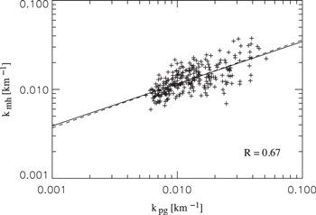
Figure 2. Wavenumber position of the magnetic helicity signature kmh as a function of the inverse proton gyroscale  The ordinary least-squares fit (solid line) is given by the formula
  The robust fit
  is shown as a dashed line for reference.
Download figure:
Standard image High-resolution imageFigure 2 also displays the iteratively reweighted least-squares fit. As can be seen from Figure 2 and the subsequent figures, the results of the robust and the ordinary least-squares regressions turn out to be almost the same. This is an indication that the least-squares method is reasonably well suited to our case.
We now compare the effects of the proton and electron thermal pressure on the magnetic helicity. For this purpose, we introduce the inverse electron pressure scale  The scale is based on the electron temperature and the proton mass. We also assume that the electron and proton densities are equal. This is justified because the relative abundance of the alpha particles generally does not exceed 5% and is not likely to make a noticeable difference. The wavenumber position of the helicity signature kmh as a function of kep is shown in Figure 3. The correlation coefficient R = 0.65 is about as high as in the case of the protons, but the dependence is somewhat stronger, the power-law slope is 0.67.

Figure 3. Wavenumber position of the magnetic helicity signature kmh as a function of the inverse electron pressure scale  The ordinary least-squares fit (solid line) is given by the formula
  The robust fit
  is shown as a dashed line for reference.
Download figure:
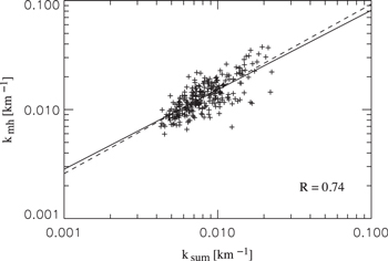
Standard image High-resolution imageNumerical simulations of Markovskii & Vasquez (2016) showed that the wavenumber position of the signature is controlled by a combined proton and electron pressure rather than by the protons or electrons alone. The wavenumber was expressed in terms of the inverse proton inertial length, and its higher (lower) value corresponded to a smaller (larger) βp + βe. This can be tested against the observational data. Figure 4 displays kmh as a function of the inverse combined pressure scale  The resulting dependence, with a power-law slope of 0.73, is stronger than in the case of the protons, and the correlation coefficient R = 0.74 is high.
Figure 4. Wavenumber position of the magnetic helicity signature kmh as a function of the inverse combined pressure scale  The ordinary least-squares fit (solid line) is given by the formula
  The robust fit
  is shown as a dashed line for reference.
Download figure:
Standard image High-resolution image
The 95% confidence intervals for the Pearson correlation coefficients given our sample of 274 elements are as follows. For the protons alone, R = 0.67 and the interval is 0.6–0.73. For the electrons alone, R = 0.65 and the interval is 0.58–0.71. For the protons and electrons combined, R = 0.74 and the interval is 0.68–0.79.
Unlike the Pearson R, the Kendall τ coefficient is nonparametric, it does not depend on the assumption of a power-law (or any other) scaling, e.g., Kendall & Gibbons (1990). For the scatter plots in Figures 2–4, the values of τ are 0.48, 0.46, and 0.55, respectively. We have tested the null hypothesis for these coefficients. The p-values associated with their deviation from zero are lower than  Therefore, the correlation is present in all three cases.
We have also carried out the Chow test (Chow 1960) to verify that the ordinary least-squares fits in the cases of the protons alone, the electrons alone, and the protons and electrons combined are different. The corresponding p-values are  or lower. This means that the differences are statistically significant.
Although the power-law slope increases when the electrons are taken into account, we were unable to show that the observed dependence is the same as in our numerical simulations, which suggest a power slope equal to 1. Most likely, this is because other processes affect the helicity, in addition to the two-dimensional turbulence modeled in the simulations. Note that the combined thermal pressure does not include the alpha particles. They can contribute to the pressure during some solar wind intervals, but on average we do not expect the contribution to be significant. If we assume that the relative abundance of the alpha particles is 5%, their temperature is four times the proton temperature, and the electron and proton temperatures are equal, then the effect of the alpha particles will be around 10%.
4. CONCLUSIONS
We have performed a statistical study of the observed magnetic helicity signature in the solar wind. The peaks of the selected signatures were well separated from the high-frequency region where the magnetic power spectrum flattens with respect to a power law. The spectral flattening is most certainly an artifact produced by the instrument. However, when the helicity is reduced considerably from its peak value before the onset of the flattening, the instrumental artifacts are unlikely to interfere with the helicity signature. In particular, aliasing, which is caused by the termination of the spectrum at the high-frequency end, appears to be insignificant.
We have analyzed the effect of electron thermal pressure on the signature position in the wavenumber space. The contribution of the electrons proves to be comparable to that of the protons. The dependence of the position on the inverse characteristic length of the electron pressure is even somewhat stronger than on the inverse proton gyroradius. Here the electron characteristic length is composed of the electron temperature and the proton mass. The correlation is high in both cases, making the dependence statistically significant.
Most importantly, we have shown that the dependence of the signature position becomes stronger yet when the inverse characteristic length corresponds to a combined pressure based on a sum of the electron and proton temperatures. The slope of the power law changes substantially from Figures 2 to 4. The correlation coefficient is also high in this case. This is in agreement with the numerical simulations carried out by Markovskii & Vasquez (2016). They found that the position of the signature is controlled by a total thermal pressure rather than by the protons or electrons alone.
As suggested by Markovskii & Vasquez (2013a), (2013b), the generation of the magnetic helicity is associated with increasing compressibility of the strongly nonlinear turbulence at smaller kinetic scales. The helicity is determined by the compressional component of the magnetic field fluctuation parallel to the mean field. The relationship between the magnetic field and density results from the assumption that the turbulent fluctuations are nearly pressure balanced, i.e., the fluctuation of the total thermal and magnetic pressure is negligible. The present analysis confirms this interpretation: if the interpretation is correct, the helicity should depend on the combined thermal pressure more strongly than on the pressure of the individual species, as demonstrated here.
The Wind spacecraft data were obtained from CDAWeb (http://cdaweb.gsfc.nasa.gov). The authors are grateful to the Wind/IMF and Wind/SWE teams for making the data available. The authors also thank the anonymous consultant statistician for helpful suggestions to improve the manuscript.
This work is supported by NSF SHINE grant AGS1357893. C.W.S. is funded by Caltech subcontract 44A-1062037 to the University of New Hampshire in support of the ACE/MAG instrument.