


ABSTRACT
Physics-based numerical coma models are desirable whether to interpret the spacecraft observations of the inner coma or to compare with the ground-based observations of the outer coma. In this work, we develop a multi-neutral-fluid model based on the BATS-R-US code of the University of Michigan, which is capable of computing both the inner and outer coma and simulating time-variable phenomena. It treats H2O, OH, H2, O, and H as separate fluids and each fluid has its own velocity and temperature, with collisions coupling all fluids together. The self-consistent collisional interactions decrease the velocity differences, re-distribute the excess energy deposited by chemical reactions among all species, and account for the varying heating efficiency under various physical conditions. Recognizing that the fluid approach has limitations in capturing all of the correct physics for certain applications, especially for very low density environment, we applied our multi-fluid coma model to comet 67P/Churyumov–Gerasimenko at various heliocentric distances and demonstrated that it yields comparable results to the Direct Simulation Monte Carlo (DSMC) model, which is based on a kinetic approach that is valid under these conditions. Therefore, our model may be a powerful alternative to the particle-based model, especially for some computationally intensive simulations. In addition, by running the model with several combinations of production rates and heliocentric distances, we characterize the cometary H2O expansion speeds and demonstrate the nonlinear dependencies of production rate and heliocentric distance. Our results are also compared to previous modeling work and remote observations, which serve as further validation of our model.
Export citation and abstract BibTeX RIS
1. INTRODUCTION
Comets are believed to preserve the pristine building materials from when the solar system was formed about 4.5 billion years ago. In addition, they may also have a role in the origin of water and organics necessary for life on Earth, according to some theories. Therefore, they are natural laboratories to test various hypotheses on the most fundamental questions about our solar system and the emergence of life. The absolute or the relative abundances of some important chemical compounds (H2O, CO, CO2, etc.) and their total amounts in a comet are observed and watched closely. In situ measurements have been performed on or near comets within hundreds of kilometers by a handful of space missions, while most observations are carried out by telescopes remotely in wavelength ranges from X-ray to radio. Because remote observations of chemical composition are made of gas in the coma, an understanding of the complicated photo-chemistry and gas dynamics in the cometary environment is needed to interpret measurements. Therefore, numerical models based on first principles are in demand to understand the changing physical conditions in the coma that are observed on different comets at various cometocentric distances or different heliocentric distances.
There are mainly two types of numerical cometary gas models. One is based on the fluid approach and the other one is based on the kinetic/particle approach. The Direct Simulation Monte Carlo (DSMC) method, as one of the typical particle approaches, provides a solution to the Boltzmann equation by tracking the microscopic quantities, i.e., velocity and location of every particle. If the number of particles is large enough to minimize the statistical error, one can derive macroscopic quantities, (e.g., density, bulk velocity, and temperature) from the statistics of the microscopic quantities of the modeled particles. The particle or kinetic approach does not make any assumption on the distribution function which the Boltzmann equation solves, while the fluid approach is derived by taking moments of the Boltzmann equation and is often under the assumption that the distribution function does not deviate too far from the Maxwellian distribution, which assumes a collisionally dominated regime. One practical limitation of the particle DSMC solution to the Boltzmann equation is that computational resources usually limit complicated 3D problems to solving for steady-state conditions. The limitation of the fluid approach is that, while the coma may be dense and highly collisional near the nucleus, by thousands to millions of kilometers away it becomes rarefied and almost collisionless.
The Knudsen number serves as a criterion to check the validity or the applicability of a fluid model. It is the ratio of the mean free path λ to the length scale of the gas,  . It is often believed that if Kn is less than 0.1, the collision is frequent enough so that the distribution function can be still approximated by a Maxwellian (Marconi et al. 1996). Crifo et al. (2003) also showed excellent agreement between their single-fluid gas dynamic model based on Navier–Stokes equations and their DSMC model for a low production rate of about 1023 s−1 and a Knudsen number up to 1. As the Knudsen number in a real cometary environment may have a wide range, the fluid approach is only physically correct in a limited region, while the kinetic approach can be applied to the whole domain. However, when it comes to modeling a bright comet or a time-dependent phenomenon, it is computationally expensive to simulate a large number of particles, because the small mean free path severely limits the time step.
In addition to the dynamics, the photo-chemistry plays an important role in the coma as well. Photochemical reactions not only alter the composition, but also fuel the coma with their released excess energies. One major reaction for H2O is  . When one H2O molecule dissociates, its daughter species H and OH are born, with average speeds of 17.5 km s−1 and 1 km s−1, respectively. The additional kinetic energy is provided by the excess energy ΔE = 1.7 eV. Due to the conservation of momentum, the H atom has a speed 17 times that of OH molecules. If the gas density is high, these superthermal H atoms will be thermalized after plenty of collisions with other atoms and molecules. In this process, the kinetic energy of the superthermal H atoms will be transformed to thermal energies and will be redistributed among all species. If the gas density is low, the superthermal H atom escapes before enough collisions take place, resulting in a lower heating efficiency. Therefore, models based on the fluid approach should take into account the photochemical heating source in the energy equation, but the heating efficiency should vary with the gas density.
Various methods have been used to address the photochemical heating efficiency. Ip (1983) derived an analytic estimate for the photochemical heating source, which is a function of H2O density and cometocentric distance. Huebner & Keady (1983, pp. 165–183) divided the computing domain into several shells and calculated the escape probability of the H atom and the energy deposited in each shell. The 1D multi-fluid model by Marconi & Mendis (1983) simulated two populations of H atoms: one is thermalized and the other one is superthermal. In their model, the superthermal atoms produced by photo-dissociation do not have the pressure or energy equation. They are lost at the collision rate with heavy species, while thermalized atoms are generated at the same rate. The resulting thermalized atoms tended to have a temperature close to that of water. Later, several hybrid kinetic/fluid models were developed (Combi 1987; Ip 1989). They used Monte Carlo models to provide the heating efficiency to the fluid model. A pure particle model, typically the DSMC approach (Tenishev et al. 2008), can treat the system in a more straightforward way. Collisions between particles and photo-dissociations in the model mimic the physical processes in nature.
In this work, we develop a 3D multi-fluid model, which treats H2O, OH, H2, O, and H as separate fluids and each fluid has its own density, velocity, and temperature. Photochemical reactions and collisions are included. Collisions between fluids allow different gases to exchange momentum and energy. The collision frequency is proportional to the gas densities of both interacting species, so the model is able to address the heating efficiency issue in a self-consistent way. In the following section, we will first describe our model in detail and then compare our results on comet 67P/Churyumov–Gerasimenko with that from a DSMC model (Tenishev et al. 2008). In addition, the fluid approach is computationally efficient enough to be able to be applied to more complicated time-dependent problems and not limited to steady-state solutions. We demonstrate that despite the various approximations, the multi-fluid model is able to produce generally similar results to the DSMC approach on a large length scale up to 106 km, which makes it a useful and computationally less demanding alternative to the particle approach. Finally, we present a more general study of the effects of the production rate on the expansion speed and the temperature of H2O, which we then compare with radio telescope observations of over 30 comets from Tseng et al. (2007).
2. METHODOLOGY
2.1. Model Description
Our multi-fluid model solves a set of hydrodynamic equations for each species, which are shown in Equations (1)–(3). They are the continuity equation, the momentum equation, and the pressure equation. ρs,  , ps are the mass density, the velocity vector, and the scalar pressure of the neutral species s. γs denotes the specific heat ratio of species s. The terms on the right-hand side of the equations represent the source terms, which are specified for each species and include collisions, chemical reactions, and the excess energies accompanied by photo-dissociations.


The source terms are described in Equations (4)–(7). Those source terms with chemical reaction frequencies  are related to photochemical reactions. The photochemical reactions, reaction rates, and the corresponding excess energies used in the model are shown in Table 1. In the pressure source term, the excess energies are partitioned under the restriction that the momenta of the daughter species should be conserved and thus are inversely proportional to the mass. The source terms involving momentum transfer coefficients
  between species s and t are terms accounting for collisions. The collision frequency is linearly proportional to the density of each involved gas species, and the relative speed of the colliding gas molecules or atoms, which is calculated from the thermal and bulk velocities of both species. The cross sections for the modeled collisions are also listed in Table 2. We note here that cross sections of self-collisions are not included, since fluid approaches assume an approximately Maxwellian distribution for each fluid, implying plenty of self-collisions in the gas of the species. To account for the infrared cooling effect of H2O, a cooling function L is added to the pressure source term of H2O. L is expressed as
  erg cm−3 s−1, which was first proposed by Shimizu (1976), and works well for the cases in this paper. But it needs additional adjustment involving optical depth for production rates higher than 1030 s−1, since the inner coma under such circumstances is optically thick, preventing efficient radiative cooling. The adjusted cooling rate can be found in Gombosi et al. (1986), which does not make much difference for the cases shown here compared with more complex approaches that account for the non-LTE effects between kinetic and rotational temperature (Combi 1996; Tenishev et al. 2008).
We note here that collisions in our model conserve momentum and energy. The sums of the collisional sources of momentum and energy of two colliding fluids are zero. However, the pressure sources rather than the energy sources are presented here, because the collisional terms in pressure equations are more concise and clear.
Table 1. Chemical Reactions and Corresponding Parameters
| Wavelength (Å) | Reaction | Reaction Rate (s−1) | Excess Energy (eV) |
|---|---|---|---|
| 1357–1860 | H2O + hν  H + OH H + OH |
8.0 × 10⁻⁶ | 1.7 |
H2O + hν  H2 + O H2 + O |
8.4 × 10⁻⁸ | 1.7 | |
| 1216 | H2O + hν  H + OH H + OH |
8.0 × 10⁻⁶ | 4.5 |
H2O + hν  H2 + O H2 + O |
2.8 × 10⁻⁷ | 1.7 | |
| 984–1357 (excluding 1216) | H2O + hν  H + OH H + OH |
3.6 × 10⁻⁷ | 4.5 |
H2O + hν  H2 + O H2 + O |
4.8 × 10⁻⁸ | 1.7 | |
| <984 | H2O + hν  ionization products ionization products |
7.0 × 10⁻⁷ | |
| 2160 | OH + hν  H + O H + O |
4.5 × 10⁻⁶ | 0.36 |
| 2450 | 5.0 × 10⁻⁷ | 0.67 | |
| 1400–1800 | 1.4 × 10⁻⁶ | 3.2 | |
| 1216 | OH (12Δ) | 3.0 × 10⁻⁷ | 3.8 |
OH ( ) ) |
5.0 × 10⁻⁸ | 1.6 | |
OH (2  ) ) |
5.0 × 10⁻⁸ | 3.8 | |
| <1200 | OH ( ) ) |
1.0 × 10⁻⁸ | 2.7 |
H2 + hν  H + H H + H |
1.1 × 10⁻⁷ | 1.8 | |
Download table as: ASCIITypeset image
Table 2. Cross Sections of Collisions for Major Components in the Comae
| Component | Cross Section (cm−2) | Component | Cross Section (cm−2) |
|---|---|---|---|
| H2O–OH | 3.2 × 10⁻¹⁵ | H2O–H2 | 3.2 × 10⁻¹⁵ |
| H2O–H | 1.8 × 10⁻¹⁵ | H2O–O | 1.8 × 10⁻¹⁵ |
| OH–H2 | 3.0 × 10⁻¹⁵ | OH–H | 1.5 × 10⁻¹⁵ |
| OH–O | 1.5 × 10⁻¹⁵ | H2–H | 1.5 × 10⁻¹⁵ |
| H2–O | 1.5 × 10⁻¹⁵ | H–O | 1.2 × 10⁻¹⁵ |
Download table as: ASCIITypeset image
Our model is based on the BATS-R-US (Block-Adaptive Tree Solar wind Roe-type Upwind Scheme) code (Powell et al. 1999; Tóth et al. 2012), which is capable of solving the magnetohydrodynamics (MHD) and hydrodynamics equations efficiently on adaptive grids. The simulations are performed on a 3D spherical grid, the radius of which is 1.4 × 10⁶ km for the comet 67P case. A spherical body with a radius of 2 km is placed at the origin to model the comet nucleus. We note here that a realistic nucleus radius of comets with a production rate higher than 1030 s−1 should be more than 20 km. However, as our model shows for comets with high production rates, a realistic radius does not change the results at cometocentric distances larger than 50 km. The resolution in the radial direction is about 370 m near the nucleus and about 1.2 × 10⁵ km near the outer boundary of the computing domain. The resolutions in the polar and azimuthal directions are about 0 7 and 14. This grid allows studying the coma in different length scales but without too heavy of a computational burden. In addition to the adaptive grid, two features in the BATS-R-US code also greatly improve the efficiency and accuracy of the model. The first is the steady-state mode, where the time steps are different in every grid cell limited by the local stability condition only, so that the time to the convergence is reduced. The second is the point-implicit scheme (Tóth et al. 2012), which facilitates the calculation of the stiff source terms, which are mainly related to the photo-chemistry in the coma without spatial derivatives involved. For example, during a single computational time step, one minor species may have a density so tiny that it may be comparable to the incremental density added by the photochemical reactions. An explicit scheme cannot compute such terms efficiently and accurately, but the point-implicit scheme can handle them well.
2.2. Boundary Conditions
To compare our results with the DSMC results (Tenishev et al. 2008), we run the model to simulate comet 67P at four heliocentric distances with the same or close set of parameters as possible between fluid and kinetic models. The inner boundary condition on the surface of the nucleus for the only parent species, water, is fixed. H2O flux F and H2O temperature T are set as functions of the solar zenith angle, which is described by Tenishev et al. (2008). Following Huebner & Markiewicz (2000) and Bieler et al. (2015), the magnitude of the H2O velocity u on the surface is  , where k is the Boltzmann constant and m is the molecular mass of H2O. The velocity is normal to the surface. The number density is calculated by
  . The pressure at the boundary is set to be
  . For all other species, the photo-dissociation products of water, a floating boundary condition is set for all variables, in which a zero gradient is imposed. At the outer boundary, floating boundary conditions are also applied for all variables.
In Section 3.2, we study the effects of production rates on the coma morphology, so the inner boundary conditions are slightly modified. The flux is set to be uniform on the surface and the temperature is fixed to 180 K. The heliocentric distances are fixed to 1.0 au for all cases and we only vary the neutral gas production rate from 1027 to 1030 s−1 in these simulations.
To compare with remote observations of several comets, we run more cases with varying heliocentric distances and different production rates, and obtain the expansion speed of H2O at about 105 km from the nucleus. The distance is chosen mainly because the expansion speeds reported by Tseng et al. (2007) were measured approximately at that distance.
3. RESULTS AND DISCUSSION
3.1. Comparison with the DSMC Model
2D cuts of densities, speeds, and temperatures of H2O and H from the multi-fluid model results at 1.3 au are shown in Figure 1. The Sun is in the direction of negative x-axis. The effect of solar illumination can be seen from the H2O results. Density, speed, and temperature of H2O are higher on the dayside than the nightside. But this is not true for H. Because of more collisions taking place on the dayside, the dayside speed and temperature of H are lower. A similar picture to H applies to other daughter species.
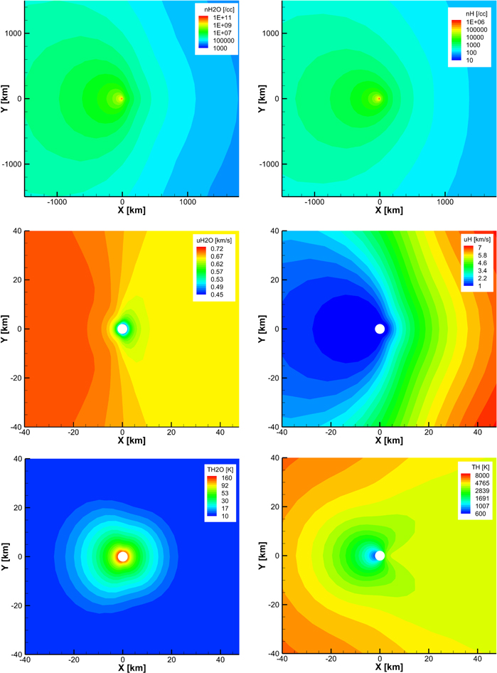
Figure 1. 2D cuts of the model results at 1.3 au with a production rate of 5 × 1027 s−1. Three rows represent densities, speeds, and temperatures of H2O (left column) and H (right column). The Sun is in the direction of the negative x-axis.
Download figure:
Standard image High-resolution imageIn this section, we will juxtapose our model results and the DSMC solution, and display the similarities and the differences between them. Specifically, the 1D profiles of velocities, temperatures, and densities of modeled species extracted along the comet-Sun line are compared. Such comparison are made at four heliocentric distances: 1.3, 2.0, 2.7, and 3.3 au with production rates of 5 × 1027, 8 × 1026, 8 × 1025, and 1 × 1024 s−1, respectively.
3.1.1. Velocity
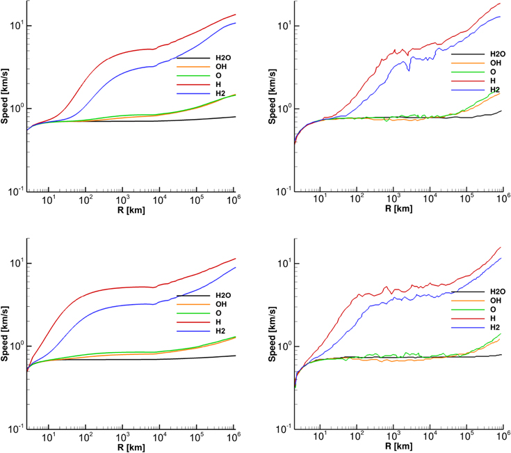
Figure 2 shows the speed of each species at four heliocentric distances, with the left column displaying our fluid model results and the right column the DSMC results from Tenishev et al. (2008). The following figures of temperatures and densities have the same format. We can spot three groups of lines in the four cases in both columns. H and H2 behave as one group, while O and OH are another one. Each group has similar masses, and gains energy from the photo-dissociation. The group of H and H2 has the highest speeds, the group of O and OH has the second highest. H2O almost stays level after a short distance of acceleration, with collisions with daughter species as its only source for acceleration. The speeds of H and H2 are decoupled from H2O before O and OH diverge from H2O at a larger distance. The decoupling distance decreases with lower production rates. This trend can be readily explained by fewer collisions in a thinner coma and more excess energy translated to the kinetic energy. Therefore, as production rate decreases, H and H2 reach the plateau of the bulk speed at about 5 km s−1 in a shorter distance, resulting in a steeper slope in the velocity profile.The new fluid and DSMC kinetic results are quite similar in all respects.
Download figure:
Standard image High-resolution image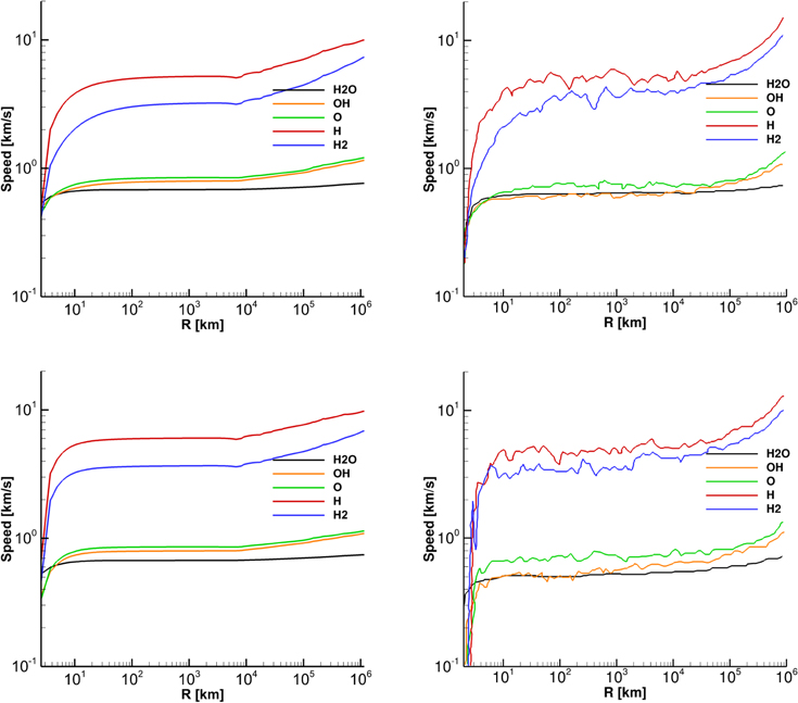
Figure 2. Speeds of modeled species vs. distances from the body. Four rows represent results for four heliocentric distances: 1.3, 2.0, 2.7 and 3.3 au. The production rates are 5 × 1027, 8 × 1026, 8 × 1025, and 1 × 1024 s−1, respectively. The left column shows our fluid model results and the right column shows the results reproduced from Tenishev et al. (2008).
Download figure:
Standard image High-resolution image3.1.2. Temperature
Figure 3 displays temperatures for all species at the selected four heliocentric distances. The temperature behavior can also be divided into the three groups mentioned in the previous section. H and H2 have the highest temperatures. OH and O are intermediate. Without any excess energy input, H2O is the coldest. The temperature of H2O decreases due to the adiabatic expansion at distances less than 100 km, then remains at the level of around 10 K. For cases with larger production rates, the temperatures of H, H2, O, and OH first drop slightly before increasing to high levels. As the drops are mainly caused by the collisions with the cold H2O, the lack of collisions for the cases with low production rates leads to the disappearance of the dips.
Download figure:
Standard image High-resolution image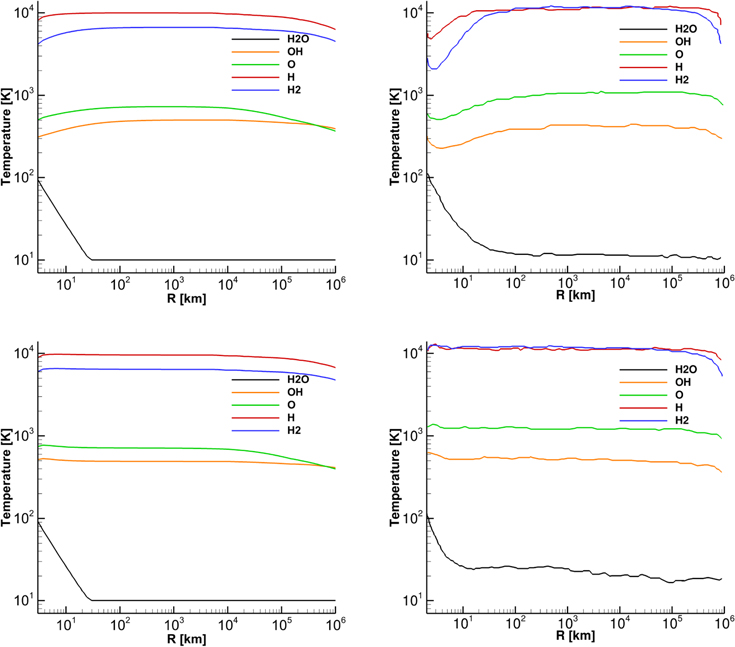
Figure 3. Temperatures of modeled species vs. distances from the body. Four rows represent results for four heliocentric distances: 1.3, 2.0, 2.7 and 3.3 au. The production rates are 5 × 1027, 8 × 1026, 8 × 1025, and 1 × 1024 s−1, respectively. The left column shows our fluid model results and the right column shows the results reproduced from Tenishev et al. (2008).
Download figure:
Standard image High-resolution imageWe also notice that temperatures of all daughter species decline at large distances. This may be for two possible reasons. The first is the cooling effect caused by adiabatic expansion. The second reason is that the relative abundance of the parent species to the daughter species decreases farther out. As a result, the percentage of newly born daughter species with a high photo-dissociation temperature drops in the population of the daughter species. The bulk temperature is thus decreased. Later we will show the relative abundance of the parent species to the daughter species also decreases faster at smaller heliocentric distances due to the shorter photo-lifetime of the parent species, which explains why in the 1.3 au case the temperatures of daughter species drop most quickly.
The most obvious difference between our fluid model and the DSMC model is the decreasing rate of the water temperature. In the fluid model results, the water temperature decreases to the minimum temperature of 10 K within 20 km for all four cases. But the slopes in the DSMC results are flatter, especially in the cases of 1.3 and 2.0 au with the minimum temperature reached at 100 km. This may be caused by the fluid model overestimating the self-collisions, so adiabatic expansion happens more efficiently than in the DSMC which yields less frequent collisions.
It is interesting to see in the DSMC results that the H2O temperature jumps to about 100 K near 106 km in the 1.3 au case. According to Tenishev et al. (2008), this is caused by the selection effect. Most of the slower H2O particles have already been destructed by photo-dissociation. We can also see that in the velocity plot, close to 106 km the water velocity goes up significantly. Due to the nature of the fluid approximation, our model is not able to include such purely kinetic effects related to distribution functions.
3.1.3. Density
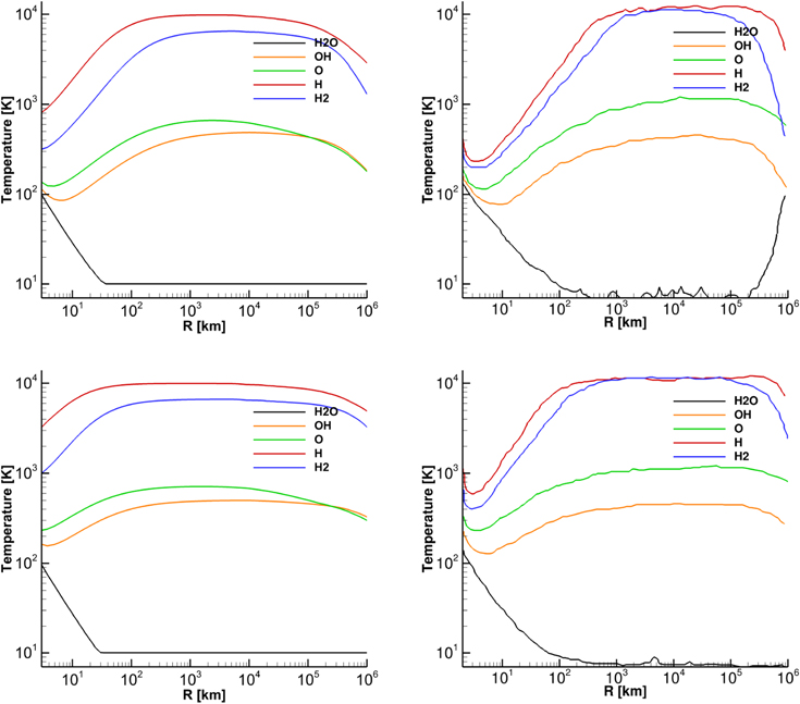
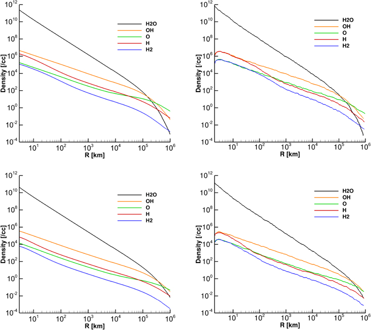
Figure 4 presents the densities of all species versus the cometocentric distances. The densities decrease almost linearly on log–log plots. The two columns look similar. H2O decreases the fastest, since it gets photo-dissociated at a high rate without any new supply. In the cases at 1.3 and 2.0 au, we can see H and OH have the same density near the nucleus and diverge after some distance. The explanation is that they are produced by the same chemical reaction and they share the same velocity in the collisional region. Outside the collisional region, freshly produced fast H dominates compared with slower OH. As a result, the H density declines faster. In other cases, while even in the vicinity of the nucleus is collisionless, the H density is lower than OH all the way out. The same reasoning also applies to H2 and O.
Download figure:
Standard image High-resolution image
Figure 4. Densities of modeled species vs. distances from the body. Four rows represent results for four heliocentric distances: 1.3, 2.0, 2.7 and 3.3 au. The production rates are 5 × 1027, 8 × 1026, 8 × 1025, and 1 × 1024 s−1, respectively. The left column shows our fluid model results and the right column shows the results reproduced from Tenishev et al. (2008).
Download figure:
Standard image High-resolution image3.2. The Effect of Production Rates
To study the effects of the production rate on coma dynamics, we run the model at 1.0 au but with four different production rates: 1027, 1028, 1029 and 1030 s−1. Figure 5 shows, for all four cases, the speed of water, the mean speed of the three heavy species (H2O, OH, O), and the mean speed of all five neutral species. The 1027 and 1028 s−1 cases are very similar in the speed profile, suggesting the role of collisional heating is negligible with a low production rate or a low density. The water terminal speed in the 1027 and 1028 s−1 cases is 0.7 km s−1, which is mainly determined by the initial temperature. As the production rate increases, the collisional heating effect kicks in. In the 1029 s−1 case, the water speed at 105 km is 0.9 km s−1 and it rises to about 1.4 km s−1 in the 1030 s−1 case. This result also agrees well with Bockelee-Morvan & Crovisier (1987). In the other two plots, we find the mean speed accelerates beyond 104 km because of the contributions by the fast species. As a result, the increase of the production rate has more impact on water speed than the bulk speeds of heavy species and all combined species.

Figure 5. The speed profile of H2O, the mean speed profile of three heavy species (H2O, OH, O), and the mean speed profile of the five neutral species at 1.0 au. The four different colors denote four production rates: 1027, 1028, 1029 and 1030 s−1.
Download figure:
Standard image High-resolution imageFigure 6 shows the temperature of H2O, the mean temperatures of three heavy species (H2O, OH, O), and the mean temperatures of all five neutral species for the four cases. In the H2O temperature profile, there is a peak beyond 104 km in the cases of 1029 and 1030 s−1 production rates. The general trend is similar to that in Bockelee-Morvan & Crovisier (1987). But the specific peak values are slightly different between our model and theirs. In the 1030 s−1 case, our peak near 140 K is higher than the peak at 110 K in their model. It may be because their model is single-fluid and treats photochemical heating and radiative cooling in a different way to ours. In the 1029 s−1 case, both models have roughly the same peak near 45 K. The temperatures in the other two plots all have dips within 1000 km but then the uptrend remains beyond 1000 km. Though the temperatures of the four cases increase at different rates, they are close to each other around 105 km. This suggests that, when the cometocentric distance is large enough, the average temperature of all gases may not vary much with the production rate. At large cometocentric distances all species become collisionally decoupled and the secondary species trend to the photo-production temperatures, which are independent of the production rates. Figures 5 and 6 illustrate the radiative cooling effect on the speed and the temperature of water. Within 1000 km, in the 1030 s−1 case, because of the most significant cooling effect caused by the highest water density, the speed and temperature are dampened for a larger distance than those in other cases.
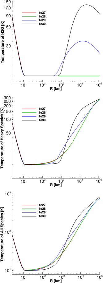
Figure 6. The temperature profile of H2O, the mean temperature profile of three heavy species (H2O, OH, O), and the mean temperature profile of the five neutral species at 1.0 au. The four different colors denote four production rates: 1027, 1028, 1029, and 1030 s−1.
Download figure:
Standard image High-resolution imageFigure 7 shows the mean molecular mass versus the cometocentric distance for varying production rates. Since the comet in this study is kept at a heliocentric distance of 1.0 au and has H2O as its only parent species, the four cases yield very similar curves. The difference in the speed profiles is the only factor capable of altering the relative abundances and thus the mean molecular mass. We can expect, if all species have fixed speed profiles for each individual species, that the four cases should have the same mean molecular mass profile. We also notice that the mean molecular masses at 105 km almost converge to a single value of about 15.4 amu.
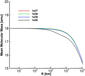
Figure 7. The mean molecular mass profiles of four production rates at 1.0 au. The four colors denote four production rates: 1027, 1028, 1029, and 1030 s−1.
Download figure:
Standard image High-resolution image3.3. Comparison with Remote Observations
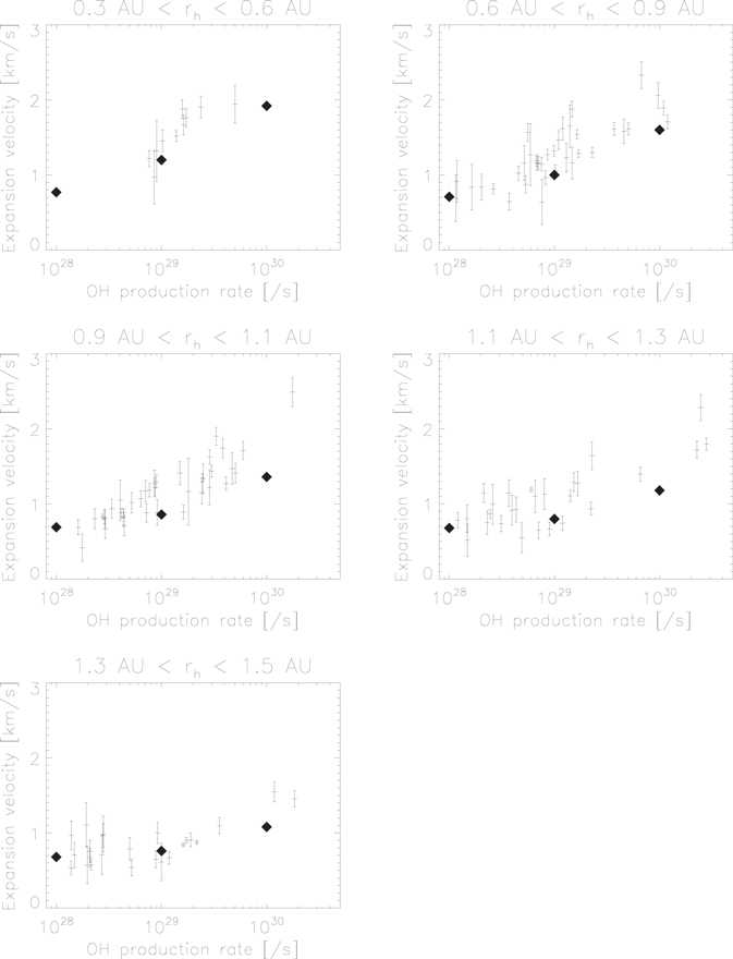
In this section, we characterize the cometary H2O expansion speeds extracted from our multi-fluid gas coma model at a cometocentric distance of 105 km. The model is run with several selected production rates and heliocentric distances. The results are listed in Table 3. One can readily see from the table that a larger production rate and a smaller heliocentric distance (i.e., a higher photon flux) lead to a higher expansion speed as expected (Combi 1987).
Table 3. H2O Expansion Speeds
| Heliocentric Distance (au) | H2O Production Rate (s−1) | ||
|---|---|---|---|
| 1028 | 1028 | 1030 | |
| 0.5 | 0.77 | 1.20 | 1.92 |
| 0.7 | 0.71 | 1.00 | 1.60 |
| 1.0 | 0.69 | 0.86 | 1.36 |
| 1.2 | 0.68 | 0.80 | 1.18 |
| 1.4 | 0.68 | 0.76 | 1.08 |
Download table as: ASCIITypeset image
Tseng et al. (2007) derived the H2O expansion speeds from the 18 cm line shapes of the OH radicals observed by radio telescopes in over 30 comets, which is reproduced in Figure 8 and serves as benchmark for our model. Our model results, which are denoted by solid diamonds, are superimposed on the observations. We note here the x-axis in Figure 8 represents the OH production rate, which is often obtained by multiplying a factor of 0.86, the photo-dissociation branching ratio of H2O to OH, with the H2O production rate (Harris et al. 2002; Combi et al. 2004, pp. 523–552). For simplicity, we assume the OH and H2O production rates are the same. Beyond 0.6 au, the diamonds in the 1028 and 1029 s−1 cases are close to each other, while the spread between the 1029 and 1030 s−1 cases is significantly larger. In the figure where the heliocentric distance is smaller than 0.6 au, the increase in production rate results in a more evenly increase in water speeds than at other distances. This reflects the nonlinear effect of the production rate and the heliocentric distance on the expansion speed, which is similar to the threshold effect mentioned by Tseng et al. (2007). In addition, the model is also applied to comet C/1995 O1 (Hale-Bopp) at the heliocentric distance of 1.0 au. The radiative cooling effect is neglected within 104 km because of the large high production rate of 8 × 1030 s−1. Our model yields similar results to that of the single fluid model in Combi et al. (1999) and Combi (2002), which matched the observations in Biver et al. (2002). It is because the production rate is so large that most heavy species are coupled within a cometocentric distance of 105 km and thus the single fluid assumption is still valid. In any case, our multi-fluid model well reproduces the observed variation in coma outflow speeds with different comet gas production rates and heliocentric distances.
Figure 8. H2O expansion speed retrieved from remote observations and obtained from our model at a cometocentric distance of 105 km. The speeds from observations are shown by vertical lines with error bars, which are reproduced from Tseng et al. (2007). The solid diamonds represent our model results.
Download figure:
Standard image High-resolution image
4. SUMMARY
In this work, we described our multi-fluid neutral gas coma model and discussed the underlying principles of coma models based on the fluid and the particle approaches. We applied our multi-fluid coma model to comet 67P at various heliocentric distances and demonstrated that it produces comparable results to the DSMC model, which is based on the kinetic approach and physically correct in all collisional regimes encountered at the comet. Therefore, our model may serve as a powerful alternative to the particle-based model, especially for computationally intensive 3D and/or time-dependent simulations. Since the model is capable of simulating the photochemical reactions and the redistribution of the excess energies via collisions among all gases, we are able to show the nonlinear relationship of production rate and heliocentric distance on the water expansion speeds. For the case at 1.0 au, when the production rate is lower than 1028 s−1, the increase in production rate will not make much difference. If the production rate is equal to or larger than 1029 s−1, H2O is accelerated and heated significantly by the hot photochemically produced daughter species, mostly atomic hydrogen. The variations in temperature and mean molecular mass along the cometocentric distances are also discussed. In addition, our results are comparable to previous model results and remote observations, suggesting validity and applicability of the model to interpret cometary observations.
The work at the University of Michigan was supported by the NASA Planetary Atmospheres grant NNX14AG84G and US Rosetta contracts JPL#1266313 and JPL#1266314. Resources for all simulations in this work have been provided by NASA High-End Computing Capability (HECC) project at NASA Advanced Supercomputing (NAS) Division.