


Abstract
Photometric and astrometric calibration of high-contrast images is essential for the characterization of companions at small angular separation from their stellar host. The main challenge to performing accurate relative photometry and astrometry of high-contrast companions with respect to the host star is that the central starlight cannot be directly used as a reference, as it is either blocked by a coronagraphic mask or saturating the detector. Our approach is to add fiducial incoherent faint copies of the host star in the image plane and alternate the pattern of these copies between exposures. Subtracting two frames with different calibration patterns removes measurement bias due to static and slowly varying incoherent speckle halo components, while ensuring that calibration references are inserted on each frame. Each calibration pattern is achieved by high-speed modulation of a pupil-plane deformable mirror to ensure incoherence. We implemented the technique on-sky on the Subaru Coronagraphic Extreme Adaptive Optics instrument with speckles which were of the order of 103 times fainter than the central host. The achieved relative photometric and astrometric measurement precisions for 10 s exposure were respectively 5% and 20 milliarcsecond. We also demonstrate, over a 540 s measurement span, that residual photometric and astrometric errors are uncorrelated in time, indicating that residual noise averages as the inverse square root of the number of exposures in longer time-series data sets.
Export citation and abstract BibTeX RIS
1. Introduction
Direct imaging of a faint companion at small angular separations from the host star is extremely difficult as the companion is obscured by the residual starlight, which forms a bright halo around the point-spread function (PSF) core. High-contrast imaging instruments such as the Gemini Planet Imager (GPI; Macintosh et al. 2014), Spectro-Polarimetric High-contrast Exoplanet REsearch (SPHERE; Beuzit et al. 2008), Magellan Adaptive Optics (MagAO; Males et al. 2018), P1640 (Hinkley et al. 2011), and the Subaru Coronagraphic Extreme Adaptive Optics (SCExAO; Jovanovic et al. 2015) have been pushing the detection limit at small angular separation (typically within 5 au for the nearest objects) from stellar hosts. These instruments share a common architecture, including one or two deformable mirrors (DM) with a large number of actuators to compensate for high-order wave front errors, wave front sensors to measure static and dynamic aberrations, coronagraphs to occult the on-axis starlight, and a highly sensitive science detector with minimal readout noise. With these existing technologies, instruments can provide high-contrast imaging capabilities delivering images and spectra of exoplanets. Accurate measurement of the exoplanet flux and position in such images is essential for orbit determination and characterization (chemical composition, mass, effective temperature). Yet, in post-coronagraphic images it becomes quite difficult to determine the relative position and intensity of a companion as the central starlight has been blocked by a coronagraph. The position of a star behind a coronagraph can be predicted using image centroid, image symmetry, and instrument feedback (Digby et al. 2006). Often astronomers measure the flux and position of the host before and after inserting the coronagraph for calibration. This leads to inaccurate measurements of the companion as the signal from the host fluctuates in time owing to variation in Strehl or background level. In addition, any drifts of the PSF behind the coronagraphic mask will be lost as well. Sivaramakrishnan & Oppenheimer (2006) address this issue by demonstrating that a regular diffractive grid placed in the pupil plane of a telescope can create a set of copies (or satellite speckles) of the host in the coronagraphic dark region to track the position of the central star behind the coronagraphic mask. This technique has been implemented in GPI to create satellite speckles for image calibration (Wang et al. 2014). The relative motion between nearby point-source and the satellites spots formed by this pupil plane grid has been used to establish companionship for Alcor b (also known as HD 116842/HIP 65477) and also constrain the properties of the companion over a shorter observation timescale than otherwise possible (Zimmerman et al. 2010). One of the limitations of this technique is that it lacks flexibility, i.e., the spatial frequency and brightness of the satellite speckles are fixed and cannot be changed without changing the pupil mask. Also there is a slight loss in total throughput before the detector as the amplitude of the pupil function is modulated. A simultaneous independent study by Marois et al. (2006) shows that a periodic phase mask or amplitude mask in the pupil plane creates off-axis copies of the primary PSF, which can be used to track the PSF position and the Strehl ratio (SR), constraining the orbital parameters precisely (Bacchus et al. 2017; Macintosh et al. 2014). Imposing a periodic phase grid on the DM provides flexibility both in terms of controlling the speckle's intensity as well as position and also can also be used to eliminate quasi-static speckles (Martinache et al. 2014). Further, the radial elongation feature of the fiducial spots in a broadband image can be used to constrain the position of the star behind a coronagraph (Pueyo et al. 2015) and correct the residual atmospheric dispersion (Pathak et al. 2016). We have deployed this feature in the SCExAO instrument to generate artificial speckles. When created with a static DM pattern, these artificial speckles interfere with the underlying speckles from the PSF halo, warping the satellite spots, reducing the accuracy with which the PSF can be located and its brightness be determined. To address this limitation, the phase of these speckles can be rapidly (>kilohertz) switched between 0 and π within a single exposure. This effectively averages the coherently interfered speckle images in time generating a single image with temporarily incoherent calibration speckles that appear to not interfere with the underlying speckle halo. Stable, high-fidelity replicas of the PSF enable an enhanced astrometric and photometric determination of the central PSF (Jovanovic et al. 2015). Thus, modulating the phase of the grid in the pupil plane is an ideal approach for improving the precision of calibration.
Although the fast modulation ensures that calibration speckles do not interfere with the underlying PSF speckle halo, the measured intensity will be the incoherent sum of the calibration speckle flux (which we seek to measure) and the pre-existing PSF speckle halo component (which is unknown). To mitigate this measurement error, the artificial speckles could be made significantly brighter than the speckles in the halo, but doing so will divert a large fraction of starlight within or nearby the high-contrast observing region, and could also disrupt other instrument functions such as wave front sensing or short-wavelength imaging. For example, the SCExAO instrument uses a large DM amplitude (∼25–50 nm) to generate satellite spots. These bright spots are still within the dynamic range of the near-infrared (NIR) integral field spectrograph (CHARIS; Groff et al. 2017), but are too bright for the visible light polarimetric imager (VAMPIRES; Norris et al. 2015), as speckle intensity is inversely proportional to the square of the wavelength (Guyon 2005). Another solution is to locate the calibration speckles in the dark part of the coronagraphic PSF halo (dark hole), allowing for their amplitude to be greatly reduced and comparable to the companion. This is critical for calibrating the flux and astrometry of faint exoplanets as the satellite speckles must be within a few orders of magnitude in brightness to avoid dynamic range issues with the detector. However fainter speckles that meet this requirement could potentially be buried under the residual starlight halo and can therefore be challenging to locate in post-coronagraphic images. So as a general point, the calibration speckle brightness is a painful trade-off between photometric and astrometric measurement accuracy and high-contrast imaging performance.
In8 this article we present a new technique to subtract the residual starlight present under the calibration speckle. We generate a pair of incoherent fiducial copies of the host in the image plane and switch two fiducial patterns between exposures to create a set of images having alternated patterns of satellite speckles. Two images (or frames) with alternating speckle patterns are then subtracted from each other to remove the slowly varying background level and yield a bias-free measurement of the calibration speckle brightness and position. In Section 2 we give a brief overview of speckle formation and discuss the need to alternate between speckle patterns. The implementation of our approach using the SCExAO-CHARIS instrument is described in Section 3. In Section 4 we discuss some of the on-sky results obtained on the stellar target β Leo. In Section 5 we conclude the article by quantifying the on-sky precision obtained for flux and position measurement.
2. Rationale
The principle behind speckle formation can be understood using Fourier optics, considering a pupil-plane diffraction grating. A periodic diffractive grid placed in the pupil plane generates speckles (or copies of the central host) in the focal plane. Figure 1(a) represents the sinusoidal phase modulation in the pupil plane of a telescope with a similar central obstruction and spiders as the Subaru Telescope. Figure 1(b) shows the corresponding focal plane image. Two or more diffraction spots (or speckles) can be seen in the focal plane, as in Figure 1(b), depending on the amplitude of the modulation. Each speckle has its own amplitude and phase. Interference between the artificial speckles generated by the phase modulation in the pupil and those in the PSF is governed by the addition of complex amplitude. The intensity of the artificial speckles varies proportionally with the square of the amplitude of the sine wave. The relative distance of the speckles from the PSF core scales with the sine wave's spatial frequency. Azimuthal rotation of the phase modulation about the optical axis rotates the spots in the image plane. The 1D sinusoidal phase map shown in Figure 1(a) can be used to generate a single pair of speckles (we do not consider here higher-order fainter spots). By adjusting the amplitude, phase, and orientation of the sinusoidal grid, speckles can be placed at a known location with a predefined contrast with respect to the central PSF. These spots are used in this work as the calibration yardstick to characterize the flux and position of the companion.

Figure 1. Sinusoidal phase modulation in the pupil plane (a) generates satellite speckles in the focal plane (b).
Download figure:
Standard image High-resolution imageSine waves can be applied as described above to generate pairs of speckles that can be used for calibration, sometimes referred to as a calibration grid. As outlined in the 1, the speckles formed by these static grids will coherently interfere with the light in the speckle halo. This will warp the satellite speckles and vary with time reducing the precision with which the astrometry and photometry of a companion can be calibrated. Therefore, more advanced dynamic speckle modulation techniques, which modulate the phase of the modulation between 0 and π at kilohertz rates, must be used to obtain temporally incoherent speckles and maximize speckle robustness. This eliminates the coherent interference between the satellite speckle and the background speckle. Jovanovic et al. (2015) have already demonstrated that there is a clear improvement of ∼2–3 times in photometric as well as astrometric stability of the satellite spots when their phases are swapped at high speed within an exposure. However there still remains an incoherent underlying background (i.e.,  in Equation (4) of Jovanovic et al. 2015), which can ultimately limit the precision of calibration. This incoherent background becomes the dominant source of error for relatively faint satellite spots. Therefore we need a dynamic quantitative measurement of the incoherent background so as to remove it from each frame for precise calibration. This measurement can be made by turning the speckle pattern on/off between exposures. Here we demonstrate the power of utilizing a dynamic speckle grid that creates incoherent speckles and allows for the background to be removed simultaneously. What follows is a mathematical description of this process.
The relative flux measurement between the companion and the host is the goal of photometric calibration (i.e., Fp/Fs, where Fp is the companion flux and Fs is the flux of stellar host). In post-coronagraphic images, Fp/Fs is derived from measurement of Fp/Fss where Fss is the measured flux of one of the satellite speckles. The grid parameters can be adjusted to provide a given contrast between the host star and the satellite speckle, i.e., Fss/Fs = c, where c is fixed for a given sine-wave amplitude. Fp/Fs can be computed as


The error in measurement of Fp/Fs is directly proportional to the error in Fp/Fss. Hence one needs to measure Fp/Fss precisely. The measured flux of the satellite speckle (or companion) is the sum of the flux from the actual speckle (or companion) and the incoherent background level and can be expressed as


where  and
and  are the measured satellite speckle and companion flux respectively, Fss and Fp are the actual satellite speckle and companion flux, Fbg and
  are the incoherent background levels at the locations of the satellite speckle and companion respectively, and SR is the Strehl ratio. In Equations (3) and (4) we have considered incoherent artificial speckles instead of a static grid that renders coherent speckles, using the later will additionally introduce a coherent mixing term.
For slowly varying quasi-static speckles, we can eliminate Fbg or  by subtracting a frame from an adjacent frame in time where the satellite speckle and companion are absent at the position where they used to be in the previous frame. This leads to the following revised equations:


Alternating the satellite speckles pattern (i.e., spatially modulating the speckle pattern so as to put them at a location different from the previous frame) for each exposure can give us an estimate of Fbg without losing calibration spots for each frame.  can be carefully estimated using dedicated advanced post-processing techniques such as spectral differential imaging (SDI) or angular differential imaging (ADI), which are not discussed in this paper. High-contrast imaging systems use a very narrow field of view (FOV) (<2'') and the SR can be assumed to be constant across the FOV neglecting off-axis and chromatic aberrations. Thus the SR can be assumed to be the same in Equations (5) and (6) to the first order. The effect of Strehl on the measured fluxes can be eliminated by dividing the two measurements as shown below.

By using two different speckle patterns, generated by a single distinct sinusoid each, and alternating them between adjacent frames, it is possible to produce all the data needed to remove the effect of the background and SR and achieve a precise relative photometry and astrometry, while maintaining calibration speckles in every science frame. Further, as a sinusoid generates at least two satellite speckles (i.e., the simplest pattern of adding satellite spots to a frame), each exposure has several calibration points that can improve precision. This can of course be scaled by adding more sinusoids to a single exposure at the expense of flux in the PSF core.
3. Implementation and Test on the SCExAO-CHARIS Instrument
We tested the modulation scheme described above on-sky with SCExAO instrument to determine the improvement in the astrometric and photometric precision. To do this, a single unique sinusoidal pattern was applied to the DM in each frame and oscillated between frames. Figure 2 demonstrates the oscillating speckles that were generated for experiments from frame to frame. Each sine wave applied to the DM generates a pair of speckles. To measure photometry and astrometry precision, we considered one of the speckles to be the companion, and the second one to be the calibration speckle. The relative error in the measurement of these two spots in each frame can give us an estimate of the error associated with Fp/Fs assuming a random background level.
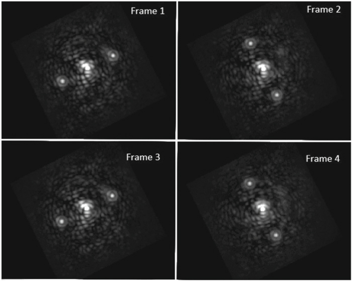
Figure 2. Images of four consecutive reduced data slices of HR8799 obtained from CHARIS at 1630 nm showing two alternate speckle patterns created by a single sine wave with an amplitude of 25 nm applied on the DM, at a separation of approximately 0 46 from the central PSF.
Download figure:
Standard image High-resolution imageThe SCExAO instrument is dedicated to high angular resolution imaging at small angular separation down to ≈1.5λ/D (where D is the diameter of the primary mirror of the Subaru Telescope). Its DM has 45 actuators across the pupil, hence satellite spots can be placed at a maximum separation of 22.5λ/D from the center. We applied a sinusoidal phase command to the DM to create speckles. In a typical observing night, we generate four bright satellite spots at a separation of 15.9λ/D from the central PSF by giving two orthogonal sinusoidal phase commands to the DM. The amplitude of the sine wave on the DM is set to be ∼25 nm or ∼50 nm. However, in order to demonstrate our new approach we generated fainter incoherent satellite speckles with brightness similar to the background speckles. Therefore, we used a sine wave of amplitude 8.8 nm (i.e.,  ) on the DM to generate speckles of a brightness eight times lower than the regular 25 nm amplitude.
On-sky data was taken on the target β Leo on the engineering night of 2019 January 12, 14:21–14:30 (UTC) with CHARIS. The average atmospheric seeing was approximately 0.3 arcsec during this period. CHARIS is an integral field spectrograph imaging the post-coronagraphic light provided by SCExAO over a 2'' × 2'' FOV. The CHARIS pixel size is 16.2 mas. CHARIS operates in the NIR wavelength region, from the J band to the K band (1160 nm to 2370 nm). The low spectral resolution mode has a resolving power (Δλ/λ) of 18.4 which covers the J band to the K band in a single shot and was used for these observations. Each CHARIS raw exposure produces a 3D data cube of 22 wavelength slices, each slide being a monochromatic 2D spatial image.
The central star was blocked by a Lyot coronagraph with an inner working angle of 113 milliarcsecond. The switching of the speckle pattern (spatial modulation) was synchronized to the CHARIS data acquisition. The exposure time of CHARIS was set to 10 s. The speckle pattern was switched between exposures, i.e., every 10 s. The phase of the sine wave on the DM during each exposure was varied (phase modulation) between 0 and π each 500 μs. SCExAO's extreme AO loop typically runs at a 2 ∼ kHz frame rate, hence the wave front sensor in SCExAO can detect this phase modulation. However, the typical loop gain is ∼0.3, so it has a much slower response time (∼200 Hz), so the fast sinusoidal phase modulation applied on the DM was uncorrected by the extreme AO loop.
The absolute contrast between the 8.8 nm speckle grid and the central PSF was measured using a laboratory super-continuum laser source stimulating the central star. CHARIS lacks a sufficient dynamic range to calibrate the contrast between the satellite speckles generated by an 8.8 nm amplitude and the central PSF. Therefore, a speckle grid of higher DM amplitude (50 nm) was used to register the relative flux between the PSF core and the 50 nm non-coronagraphic satellite speckles at first, and then the relative flux between the 50 and 8.8 nm satellite spots was computed by inserting a focal plane mask and increasing the exposure time. The spots generated by the 8.8 nm amplitude were expected to be 32 times fainter than the 50 nm amplitude. We obtained a set of eight images as presented in Figure 3 for one wavelength for absolute contrast calibration using the super-continuum laser source. This set consists of an unsaturated image of the central PSF (top left), the central PSF with the 50 nm speckles for two different speckle patterns (top middle), the 50 nm speckle grid with the Lyot coronagraph for the two patterns (top right and bottom left), the 8.8 nm speckles with the Lyot coronagraph for the two patterns (bottom middle), and an exposure with the Lyot coronagraph and no additional speckles (bottom right). We address this set of images as "ladder frames" as we acquired them in steps of decreasing order of the DM amplitude. The relative flux and position of the central PSF and the 50 nm speckle grid without any coronagraph was measured at first, and then we measured the flux and position between the 50 nm and the 8.8 nm speckle grids with the Lyot coronagraph. Using these measurements we computed the relative flux and position between the central source and the 8.8 nm speckle. The exposure with the Lyot coronagraph without any satellite speckles applied is used to subtract the background speckle halo in the coronagraphic images. Figure 4 shows the measured contrast variation of the 50 nm and 8.8 nm speckle grids as a function of wavelength. The flux ratio between the 50 nm and 8.8 nm speckle grids was measured to be ∼29. The flux ratio between the central PSF and the 8.8 nm grid at 1630 nm was measured to be ∼1.6 × 10⁻³. The flux ratio, as shown in Figure 4, is used later on to scale the average pixel counts obtained for a satellite speckle with the contrast value at a particular wavelength.
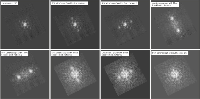
Figure 3. Classical set of ladder frames taken using the laboratory source to compute the absolute contrast between the PSF core and satellite speckles of an 8.8 nm DM amplitude.
Download figure:
Standard image High-resolution image
Figure 4. Variation of the contrast of the 50 nm and the 8.8 nm speckle grids as functions of wavelength.
Download figure:
Standard image High-resolution image4. On-sky Results
In this section we discuss results obtained on-sky on the target β Leo (A3 star type, Hmag = 1.92). The raw data were reduced using the CHARIS data reduction pipeline (Brandt et al. 2017). The level of the background speckles is much higher on-sky than in the laboratory due to the residual atmospheric wave front errors. Hence, 8.8 nm speckle spots that are clearly visible with the laboratory source are barely visible in on-sky reduced data cubes as shown in Figure 5(a). However, after subtracting two consecutive frames they can be easily located as seen in Figure 5(b). Each frame has a set of two speckles as shown in Figure 2. The relative flux and position of each speckle was measured by fitting the image of the satellite speckle to an analytical Airy disk function using a least-square fitting method. The maximum flux count, coordinates of the pixel with maximum flux, and the average flux in an annulus surrounding the image (to estimate the background offset under the fitted function) were given as initial conditions to estimate the PSF. From the fitting, we obtained the amplitude and center of the fitted function to compute the flux ratio and position coordinates of the satellite speckle with respect to the PSF core.
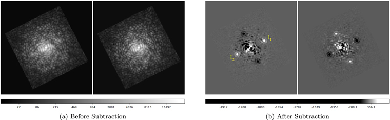
Figure 5. (a) Images of two consecutive reduced data slices of β Leo before subtraction obtained from CHARIS at 1744 nm with two alternate fainter speckle patterns where they are barely visible. (b) Images of the same data slices of β Leo after subtracting the frames from each other where the calibration speckles can be clearly seen.
Download figure:
Standard image High-resolution imageFor convenience, let the top right speckle in the left-hand panel of Figure 5(b) be I1 and the bottom left speckle on the same image be I2. Figures 6(a) and (b) show the measured flux variation of I1 without and with subtraction over a duration of 540 s at three different NIR wavelengths (J, H, and K band) with a cadence of approximately every 30 s. The exposure time for each frame was kept at 10.32 s. Figure 6(a) shows changes in the flux of I1, possibly due to variations in the SR and background. The standard deviation in the flux measurement improves after subtraction thanks to proper background subtraction, as shown in Figure 6(b). Results are summarized in the Table 1.
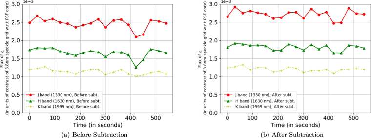
Figure 6. Flux variation of one of the speckles before (left panel) and after (right panel) subtraction. Flux is expressed in units of contrast based on static calibration from the previous Figure 4.
Download figure:
Standard image High-resolution imageTable 1. Photometric and Astrometric Precision Obtained (for 10 s Frame Exposure)
| Wavelength | Photometry (I1) | Astrometry 
|
Ratio ( ) ) |
|---|---|---|---|
| (in nm) | % Standard Deviation σ | Angular Separation (in mas) | % Standard Deviation σ |
| Before Subtraction | |||
| 1330 | 5.8 | 51 | 3.5 |
| 1630 | 7.7 | 23 | 5.2 |
| 1999 | 6.0 | 45 | 5.1 |
| After Subtraction | |||
| 1330 | 4.5 | 20 | 2.8 |
| 1630 | 4.6 | 20 | 3.7 |
| 1999 | 5.0 | 47 | 6.4 |
Download table as: ASCIITypeset image
Figure 7 shows the variation of the separation between I1 and I2 with time before and after subtraction. After subtraction, the astrometric precision significantly improves from ∼50 milliarcsecond(mas) to ∼20 mas in the J band and slightly improves from ∼23 mas to ∼20 mas in the H band. However, in the K band, due to a low signal-to-noise ratio of the satellite speckle, we did not see any improvements. These results are summarized in Table 1.
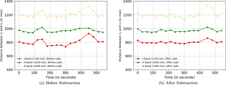
Figure 7. Distance variation between I1 and I2 with time before and after subtraction.
Download figure:
Standard image High-resolution imageUsing two alternating speckle patterns, we estimate the relative error associated with the measurement of the flux ratio between the companion and the central star. For this, we consider one of the speckle spots (i.e., I1) to be the companion and the other spot to be the calibrator (i.e., I2). Equation (7) shows that the relative error (i.e., σ) in the measurement of the ratio of intensities of I1 and I2 is equal to error in the measurement of the companion and the central star flux. Figures 8(a) and (b) show the flux ratio between speckles I1 and I2 before and after subtraction respectively. The standard deviations in measurement improve by subtracting two frames from each other for the J and H bands.  in Figure 8(a) for the J and H bands is always less than unity, suggesting that there is a bias in the measurement of
  without subtraction. Whereas, in Figure 8(b), we subtracted the underlying background sitting beneath the satellite speckle by taking two exposures with different satellite speckle patterns and measured the intensities of the clearly visible satellite spots. When we subtract two consecutive images, the common static background disappears, and the ratio is closer to unity. Since we expect the ratio between two satellite speckles to be constant over time, this indicates that even between consecutive images, the background changes by about 3.7% (H band). Assuming this background level to be random, we expect that the relative flux between the companion and central PSF can be measured to a precision of 3.7% (in the H band) using Equation (7) for a 10 s frame exposure.
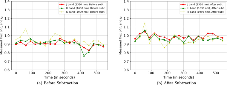
Figure 8. Ratio of intensity variation of a pair of speckle before and after subtraction.
Download figure:
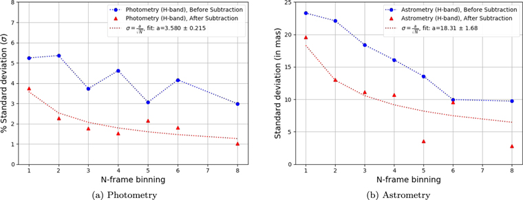
Standard image High-resolution imageWe binned N (where N is a positive integer) frames together and measured the relative flux ( ) and separation (
 ) of the resultant pair of speckle spots in each binned frame. We then computed the standard deviation (σ) in the measured relative fluxes and distances for each of the N-binned sets. Figure 9 shows the variation of the standard deviation (σ) between the measurements (before and after subtraction) with different binning numbers. In Figure 9(a), the standard deviation without subtraction (blue curve) does not converge with an increase in N, suggesting that with an increase in the number of exposures, the precision of the measurement may not improve. However, for subtracted frames (red curve) we observe that σ decreases with N in a way that is consistent with
  . This indicates that subtracting two consecutive frames has removed the biased incoherent speckle halo from
  measurements to a significant extent. Therefore, with an increase in the number data points, we expect the residual uncorrelated noise to become further negligible and obtain an unbiased precise flux measurement. Figure 9 shows a comparison of precision obtained using the regular incoherent speckle grid where we do not change the spatial pattern (blue curve) and the precision obtained by our new technique of alternating the speckle pattern (red curve). From the figure there is a clear improvement in photometric as well as astrometric precision during the same interval of time and under the same environmental conditions. For an 80 s frame exposure we can measure the relative flux between the companion and host to a precision of 1% as well as the position to a precision of ≤5 mas in the H band. Extrapolating the fitting parameters from Figure 9 to a total integration time of 1912 s, assuming similar environmental conditions, we arrive at a astrometric precision of 1.3 mas ,which is ∼2–3 times better than what has been achieved to confirm the companionship of Alcor in Zimmerman et al. (2010). The total integration time for our experiment was ∼540 s. More on-sky data is needed to perform a meaningful quantitative comparison of our technique with the previously used techniques. This will be the goal of an upcoming publication.
Figure 9. Photometric and astrometric precision with different binning numbers. (a) Photometry: variation of standard deviation in the measurement  with different binning numbers. (b) Astrometry: variation of standard deviation in the measurement of
  with different binning numbers.
Download figure:
Standard image High-resolution image
5. Conclusion
In this article we discuss the importance of satellite spots in post-coronagraphic images and the need to change their patterns for each exposure. This article provides a new approach to simultaneous photometric and astrometric calibration in the visible and NIR region using fainter satellite spots. This would be relevant to instruments such as MagAO-X (with VisAO (visible) and Clio2 (infrared) as science cameras) and SCExAO (with VAMPIRES (visible) and CHARIS (infrared) as science cameras). We considered the simplest case to demonstrate our alternating scheme, i.e., 1 kHz phase swapped sine waves in two alternating directions. The single sine-wave pair of speckles imaged on each exposure is sufficient for photometric and 2D astrometric referencing, as the star lies in the center of the line joining the spots. We deployed artificial incoherent satellite spots with alternating patterns on a high-resolution integral field spectrograph to do precision photometry and astrometry. We quantitatively demonstrated that relative flux measurements between the companion and host are insensitive to Strehl. Using this technique we determined that the relative flux between the companion and the host can be measured to an accuracy of 3.7% (for a 10 s frame exposure) in the regime where the satellite speckles and PSF halo are of similar brightness (both at ∼10−3 contrast ratio). A photometric precision of <1% and astrometric precision of <5 mas is achieved with eight-frame binning (80 s frame exposure). Using more satellite spots in a frame should improve the precision by a factor of  , where n is the number of sine waves. However, adding more satellite spots will diffract more light from the central host, which may limit the performance of the extreme AO loop. We demonstrated a practical solution to photometric and astrometric calibrations, which are challenging in high-contrast imaging. This technique is applicable for orbits, spectra, and time variation measurements from high-contrast images.
The authors acknowledge the support from Subaru Telescope, NAOJ for lending out their facility. The development of SCExAO was supported by the Japan Society for the Promotion of Science (grant-in-aid for research No. 23340051, 26220704, 23103002, 19H00703, and 19H00695), the Astrobiology Center of the National Institutes of Natural Sciences, Japan, the Mt. Cuba Foundation, and the director's contingency fund at Subaru Telescope. The work of F.M. is supported by the ERC award CoG-683029. The authors wish to recognize the very significant cultural role and reverence that the summit of Maunakea has always had within the indigenous Hawaiian community. We are most fortunate to have the opportunity to conduct observations from this mountain.
Footnotes
- 8
Based on data collected at Subaru Telescope, which is operated by the National Astronomical Observatory of Japan.