


Abstract
We identify and roughly characterize 66 candidate binary star systems in the Pleiades, Praesepe, and NGC 2264 star clusters, based on robotic adaptive optics imaging data obtained using Robo-AO at the Palomar 60'' telescope. Only ∼10% of our imaged pairs were previously known. We detect companions at red optical wavelengths, with physical separations ranging from a few tens to a few thousands of au. A three-sigma contrast curve generated for each final image provides upper limits to the brightness ratios for any undetected putative companions. The observations are sensitive to companions with a maximum contrast of ∼6m at larger separations. At smaller separations, the mean (best) raw contrast at 2'' is 3 8 (6m), at 1'' is 30 (45), and at 0
 5 is 19 (3m). Point-spread function subtraction can recover nearly the full contrast in the closer separations. For detected candidate binary pairs, we report separations, position angles, and relative magnitudes. Theoretical isochrones appropriate to the Pleiades and Praesepe clusters are then used to determine the corresponding binary mass ratios, which range from 0.2 to 0.9 in
  . For our sample of roughly solar-mass (FGK type) stars in NGC 2264 and sub-solar-mass (K and early M-type) primaries in the Pleiades and Praesepe, the overall binary frequency is measured at ∼15.5% ± 2%. However, this value should be considered a lower limit to the true binary fraction within the specified separation and mass ratio ranges in these clusters, given that complex and uncertain corrections for sensitivity and completeness have not been applied.
Export citation and abstract BibTeX RIS
1. Introduction
More than half of all stars are found in multiple star systems. As reviewed by, e.g., Goodwin et al. (2007), Duchêne & Kraus (2013), and Reipurth et al. (2014), stellar multiplicity properties appear to be set within the first few million years of a star's life. Binary frequency is observed to increase with primary star mass, from <25% for stars near the hydrogen-burning limit to >90% for stars near the top of the initial mass function. The similar distributions in mass ratio and semimajor axis for both main sequence and pre-main sequence binaries suggests that the same formation processes occur over varying core masses, and that mild core fragmentation of collapsing gas clouds is the most appropriate theory for multiple-system formation (as reviewed by Boss 1995; see also Offner et al. 2010).
In addition to having approximately the same distance from Earth, members of a star cluster form at the same time, from the same gas cloud, and have similar age and chemical composition. Thus, studying members of young clusters provides insight into star formation and evolution. A "top-down" theory describing the formation of stars in clusters invokes cloud compression and fragmentation through shocks due to supersonic turbulence. Approximately Jeans-mass fragments then collapse into single or, under further fragmentation, into binary and higher-order multiple star systems that may then undergo further subsequent dynamical evolution, including binary disruption and/or capture, as reviewed by, e.g., Goodwin et al. (2007) and Bodenheimer (2011). The "bottom-up" theory (e.g., Shu et al. 1987) describes turbulence-shocked gas that collapses directly into cores, which then become opaque to the radiation generated from conversion of gravitational energy and continue to accrete gas. These objects evolve all the way up from near the  opacity-limited fragmentation limit to become stars. In this model, binaries at
  can form at later times through disk fragmentation, if the disk is cool enough.
Binary star characteristics—such as multiplicity frequency, separation distribution, and mass ratio distribution—can support or refute different elements of the various star and multiple star formation theories, with trends in these distributions as a function of primary star mass being particularly important to quantify. Here, we examine wide-separation multiplicity in the Pleiades, Praesepe, and NGC 2264 clusters. We discuss the clusters in order of increasing distance because our observations are limited by both angular resolution (limiting detection of companions at constant photometric sensitivity) and by sensitivity (limiting the measurement of flux ratios at constant spatial resolution). Both resolution and sensitivity improve for closer targets.
The Pleiades cluster is one of the youngest and closest populous star clusters. It is well-studied and has had its constituent stars cataloged extensively (Rebull et al. 2016). The cluster has ∼1500 known members that are readily identified due to a significant common proper motion compared to background stars. From lithium depletion boundary methods, the cluster age has been determined to be 125 ± 8 Myr (Stauffer et al. 1998) while the mean distance is 136 ± 1 pc (Melis et al. 2014) and the mean extinction is often quoted as AV = 0.15 mag. Praesepe also has been extensively cataloged (Rebull et al. 2017), aided by its distinct proper motion (e.g., Adams et al. 2002; Wang et al. 2014). The ∼1000 members of Praesepe are intermediate in age, at 757 ± 36 Myr, and have a mean distance of 179 ± 2 pc (Gáspár et al. 2009) and negligible reddening. NGC 2264 is a young (∼3 Myr) cluster that is significantly further away, with a mean distance somewhere between ∼740 pc (Kamezaki et al. 2014) and ∼913 pc (Baxter et al. 2009), and a range of extinction among the ∼1500 known members. The cluster is a popular target for young star studies because it has moderately low extinction along the line of sight, and is next to a molecular cloud complex that reduces contamination from background stars.
As for exoplanet populations work, stellar multiplicity studies are conducted using techniques that sample different portions of the mass ratio  versus semimajor axis a parameter space. Spectroscopic monitoring can detect radial velocity variations from either one or both stars. Photometric monitoring is used to search for eclipses. Both methods sample close-in orbits, or small values of a, more readily than larger values of a. Direct imaging, the method employed here, samples only larger a values. All detection methods are most sensitive to binaries that have small differences in mass/size/brightness; these methods become less sensitive toward lower-mass, smaller, and fainter companions. Previous multiplicity work on the particular clusters we have investigated includes radial velocity, eclipse, and direct imaging studies, as well as photometric identification of binaries.
Among both Pleiades and Praesepe cluster members, the binary fraction is found to be higher for the more-concentrated members (Raboud & Mermilliod 1998a, 1998b), which is attributed to the general trend of increased multiplicity toward higher-mass stars, which are more centrally concentrated than lower-mass stars, perhaps because their multiplicity increases the system mass and hence shortens the timescale for mass segregation (van Leeuwen 1983).
In the Pleiades, Bettis (1975), Jaschek (1976), Stauffer et al. (1984), Pinfield et al. (2003), and Lodieu et al. (2012) assessed multiplicity based on photometric binary candidates, collectively covering spectral types A through L. Pinfield et al. (2003) concluded that the binary fraction increases toward lower masses, while Lodieu et al. (2012) used this technique to find a brown dwarf binary frequency of about 24% within 100 au. These results have significant tension (at the factor of 2–3 level) with the direct imaging results covering the same mass and separation ranges that are discussed below. Previous and new radial velocity measurements of BAFG stars were used by Mermilliod et al. (1992, 1997) and Raboud & Mermilliod (1998a) to characterize multiplicity, resulting in a ∼25% spectroscopic binary fraction, consistent with the field star population. Adaptive optics direct imaging of G and K dwarfs was used by Bouvier et al. (1997) to estimate a binary fraction of 28 ± 4% between 11 and 910 au, consistent with the field star population. Martín et al. (2000), Bouy et al. (2006), and Garcia et al. (2015) all used HST to search for binaries among small samples of brown dwarfs, finding results consistent with the low binary fraction of ∼15% or less in the field for the mass and separation range. Notably, the majority of their newly resolved systems had been identified previously as photometric binary candidates (Raboud & Mermilliod 1998a). Richichi et al. (2012) identified several Pleiades binaries from lunar occulation observations.
In Praesepe, Bettis (1975), Jaschek (1976), and Pinfield et al. (2003) identified photometric binary candidates in this cluster as well. Bolte (1991) confirmed the early candidates as true binaries via spectroscopy. Later, Boudreault et al. (2012) and Khalaj & Baumgardt (2013) addressed multiplicity in a statistical sense, with the latter authors measuring a multiple fraction of 8.5 ± 1.6% and then claiming a true binary+triple fraction of 35%. Radial velocity measurements were used by Mermilliod & Mayor (1999) to measure spectroscopic binary orbits for FGK stars. A direct imaging search for multiplicity was conducted by Bouvier et al. (2001), who estimate a binary fraction of 25 ± 5% among G and K stars between 15 and 600 au, in agreement with the field. Patience et al. (2002) surveyed B through M stars, and found a smaller binary fraction over the same separation range; however, they also had a smaller sample. Peterson & White (1984) and Peterson et al. (1989) identified several new Praesepe binaries from lunar occulation observations.
In NGC 2264, there have been few dedicated binary studies. Recently, Gillen (2015) and Gillen et al. (2017) conducted a successful search for eclipsing systems, and Kounkel et al. (2016) has identified spectroscopic binaries.
The overall conclusion from the above, as well as other papers on binarity in clusters, is that the dense cluster binary statistics are similar to the field star population binary statistics. This is in contrast to the results for young loose associations, which appear to have higher binary fractions, and lends support to the idea that the majority of the field star population were formed in clusters rather than in looser associations. An alternate hypothesis is that some binaries in young associations break up during their pre-main sequence evolution.
2. Sample Selection for Binary Search
The input samples for our adaptive optics direct imaging companion search were selected as described below. A primary consideration was the availability of high-cadence and high-precision photometric data sets (either available at the time, or pending) for likely members of each cluster. All potential targets were within the brightness range J ≈ 10–135, selected as such via 2MASS photometry. From the input samples, the robotic scheduler for Robo-AO (Riddle et al. 2014) chose the actual targets of observation, as described below.
In NGC 2264, we included the 100 brightest classical T Tauri stars and the 100 brightest weak-line T Tauri stars that have time series data from CoRoT. The CoRoT sample selection and results are described in, e.g., Affer et al. (2013), Cody et al. (2014), Sousa et al. (2016), Lanza et al. (2016), Venuti et al. (2017), and Guarcello et al. (2017).
For the Pleiades and Praesepe clusters, the stars come from the K2 open clusters investigation of J. Stauffer (program IDs GO4032 and GO5032), which aimed to completely survey the bona fide members of these two clusters with high-precision, high-cadence optical photometry. The K2 time series sample selection and resulting data are described in detail in Rebull et al. (2016) for the Pleiades, and in Rebull et al. (2017) for Praesepe. Pleiades stars were selected from the samples provided in Stauffer et al. (2007) and Bouy et al. (2015). Praesepe stars were compiled from the work of Jones & Cudworth (1983), Jones & Stauffer (1991), Klein-Wassink (1927), and Kraus & Hillenbrand (2007).
We obtained Robo-AO data for a total of 120 NGC 2264 members, 212 Pleiades members, and 108 Praesepe members. Knowledge regarding stellar multiplicity or lack thereof can inform the CoRoT and K2 lightcurve analysis.
3. Robo-AO
3.1. Hardware and Operation
Robo-AO (Baranec et al. 2014) was mounted on the Palomar 60 inch (1.5 m) telescope before being moved to the Kitt Peak 2.1 m telescope (Salama et al. 2016; Jensen-Clem et al. 2017) in 2015. At Palomar, the instrument was capable of imaging more than 200 objects per night.
Robo-AO is the first autonomous laser AO system (Baranec et al. 2014). It uses a 10 W ultraviolet laser for a guide star, which releases a 35-nanosecond laser pulse every 100 microseconds, and records the Rayleigh-scattered, returning photons to determine the correction (Riddle et al. 2015). The laser pulse is focused at 10 km. Wavefront aberrations are sampled at 1.2 kHz, which is sufficient to measure and correct the wavefront errors of the Palomar 1.5 m telescope. The 44'' field-of-view of the Robo-AO visible camera is contained within the well-corrected diffraction-limited image area.
Besides the laser-launch system, the instrument consists of the following: a set of support electronics; a Cassegrain instrument package that houses a high speed electro-optical shutter, wavefront sensor, wavefront corrector, science instrument, and calibration sources; and a single computer that controls the entire system. A master sequencer to control hardware subsystems creates an efficient overall observing system.
A queue-scheduling program selects Robo-AO targets, optimizing the desired science targets among the practical constraints. A robot sequencer points the telescope and configures the associated system. A laser acquisition process involves a search algorithm to move the uplink steering mirror; the entire instrument configuration takes less than 30 s after telescope slew. During observations, telemetry is used to maintain focus and detect drops in laser return to continually adapt to conditions. Data are stored and processed in a computer system separate from the instrument control (Baranec et al. 2014). An Andor iXon DU-888 EMCCD images the science field at 8.6 Hz (116 msec per individual frame), with the images being saved in data cubes for later processing.
The Robo-AO system can be used to build a sizable sample of moderate-contrast, diffraction-limited images of stars within just a few nights.
3.2. Data Acquisition and Image Processing
Images of 446 targets in our three clusters were collected using the Robo-AO system on 2014 November 7–11 and 2015 March 3. Either an SDSS i' filter or an LP600 long pass filter with a 600 nm cut-on was used. The latter was employed for sources fainter than R ≈ 13m on account of its increased filter breadth but similar effective wavelength.
The observing sequence for a single target, described in detail in Baranec et al. (2014), begins with a queue-scheduling program that optimizes among scientific priority, slew time, telescope limits, prior observing attempts, and laser-satellite avoidance windows. The science camera, laser, and adaptive optics system are configured as the telescope slews. Once pointed at the new target, the laser is acquired by a search algorithm that moves a steering mirror, the adaptive optics system is started, and an observation is performed with no adaptive optics correction to estimate seeing conditions. Once the laser is acquired, the adaptive optics correction is started, removing residual atmospheric wavefront aberrations at 100 Hz using a 12 × 12 actuator deformable mirror.
Total exposure times were either 120 s or 300 s, depending on source brightness. The raw data files consist of multiple data cubes of visible camera frames generated at 8.6 Hz. When a cube reaches a size of 1 GB (about 256 frames), it is closed and a new cube is generated. In a 120 (300) s exposure, about 1032 (2580) individual frames are generated.
The Robo-AO image processing pipeline is described in detail in Law et al. (2014a, 2014b). Each of our images was dark-subtracted, flat-fielded, and tip-tilt-corrected. Tip-tilt image motion was corrected using an object brighter than ∼16m in the science image field, with a post facto shift-and-add routine in the pipeline; in the case of our observations, the tip-tilt star was the main target. The images from each data cube were then stacked into a composite image with an up-sampled plate scale of 21.55 mas pixel−1.6 The data pipeline can select only a percentage of the best-quality frames for inclusion in the final image (as is done with so-called "lucky imaging"). In practice, however, all Robo-AO frames are used to produce the final output science image.
Image cutouts of 400 × 400 pixel2 (about 86 by 86), centered on each target star, were made for the subsequent analysis steps. Next, a locally optimized point-spread function (PSF) was created for each target, from at least 20 sources observed nearby in time and airmass to the target. The reference PSF images were other science images taken temporally close to the science observation (within 1–2 hr); any drift in the PSF during a night should be slow. The target PSF is modeled using a linear combination of the reference PSFs (employing the LOCI algorithm; Lafrenière et al. 2007). If a reference PSF does not correlate with the target PSF, the algorithm does not include it in the model.
This empirical PSF was subtracted from the target stacked image cutout, and both it and the remainder image were saved along with the cutout. Figure 1 illustrates a PSF-subtraction sequence.
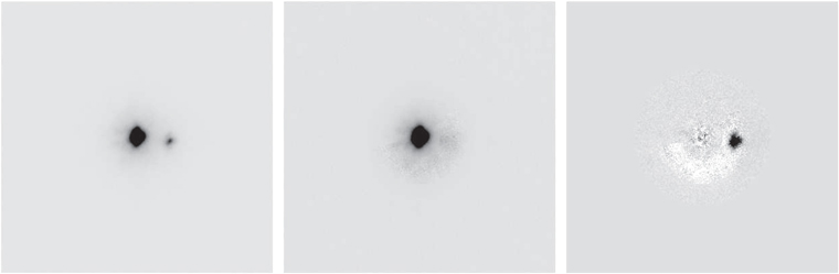
Figure 1. Shown here are the stacked image cutout (left), the PSF image assembled from images surrounding the leftmost image in time (center), and the PSF-subtracted remainder image (right) that isolates the secondary star for AK IV-314, a binary system having separation 10. North is up and east is to the right.
Download figure:
Standard image High-resolution imageWe note that, in some images, artifacts from the data acquisition and processing produced apparent "triple systems" that are identifiable because of their linear alignment on the image. Software was used to remove this effect, but it failed for some targets (<1% of the sample) and they had to be discarded from further analysis.
Each good final image stack contains either only a single source or a detected candidate binary pair. For most of the targets, the stacked image cutout allowed us to identify, measure separations and position angles, and photometer the binary components. However, in cases where the secondary star is at high enough contrast or is intrinsically too faint to be detected in the initial cutout, the PSF-subtracted image can be used to determine multiplicity and measure the properties of the secondary.
3.3. Image Quality Analysis
Image quality was used to assess the performance of the AO system and to determine the significance of the point sources detected in an observation.
We modeled the primary PSF on each image to assess image quality and monitor its variation across the data set. High-quality images have smaller FWHMs and are produced when the AO correction delivers a diffraction-limited PSF. Larger FWHM images occur when the PSF is dominated by uncorrected atmospheric turbulence, or poor seeing. Due to the image registration process, in cases of exceptionally poor correction, a single, bright, central pixel results from the stacking of seeing limited images (see discussion in Law et al. 2014a). To find the FWHM of each stacked cutout image, we fit curves with different functional forms to the flux profile; examples are shown in Figure 2.

Figure 2. Example PSF models, evaluated at whole pixel values and matched to cuts across Robo-AO image data. Left: 2D Moffat model of source BPL 167. Because the peak of the model is not located at the center of a pixel, and partial pixel values are interpolated in the plot, the peak is not well-represented graphically but is better estimated numerically. This model matches the image wings, but slightly overestimates the FWHM in the image core. Right: 2D Gaussian model of source CSIMon-0722. Relative to the Moffat model, the Gaussian model better matches the FWHM in the image core, but is worse in the image wings.
Download figure:
Standard image High-resolution imageWe first fit two-dimensional Moffat functions, using the form
where xo and yo describe the centroid position, x and y are the spatial coordinates on the image, and A, γ, and α are free parameters. Following the profile fit, its FWHM was defined as
In any given image, the number of pixels at essentially the background sky level far exceeds the number of pixels with significant amounts of flux, so we restricted the fitting box size around the primary. However, the Moffat fit failed to produce sensible results if the wings of the PSF were not entirely captured. We thus began with a 10 × 10 pixel ( ) box and incremented the box side length in steps of five pixels, until a minimum FWHM was found. Based on visual examination, the Moffat fits tended to overestimate the FWHM. For some very faint sources, however, the FWHM was underestimated because the error term used to constrain the Moffat fit did not interpolate between pixels, greatly exaggerating the image peak.
We next fit two-dimensional Gaussian functions, using the form
with free parameters  . The FWHM is then
As for the Moffat fitting, the box size for the Gaussian fit was restricted. An additional challenge for the Gaussian fitting was that too few points could be considered when fitting the model. We thus began with a fitting box of length four times the Moffat-derived FWHM, and decremented it one pixel at a time until the rms of the residual error of the centroid coordinate and its eight neighbors was below 0.1; we limited the box size to a minimum of 10 × 10 pixels.
Figure 3 illustrates the relationship between FWHM and source brightness derived under each model; Moffat fits are systematically larger than Gaussian fits. Figure 3 also illustrates the FWHM distribution in arcsec and demonstrates that the images are, for the most part, diffraction-limited. The vast majority of estimated FWHMs are 3–10 pixels, or 007–022, with a minority in a tail extending to outliers as high as 50 pixels, or 11, which implies negligible AO correction for these several objects. However, given that the diffraction limit of the Palomar 60 inch telescope at Robo-AO wavelengths is  , or ∼5.5 pixels, FWHM values less than this (formally
  ) are spurious; these are attributed to the image stacking process, which can enhance a central peak noise spike for low signal-to-noise sources. The underestimated FWHM values are not important for the photometry, which used a diffraction-limited aperture. The rise in FWHM with source brightness is expected, as the size of the PSF would increase. However, there is also a group of dimmer stars with unexpectedly large FWHMs, which we attribute to the AO correction not working as well due to the faintness of the stars, poor seeing, or possibly telescope motions—all of which can spread out the PSF of fainter objects.
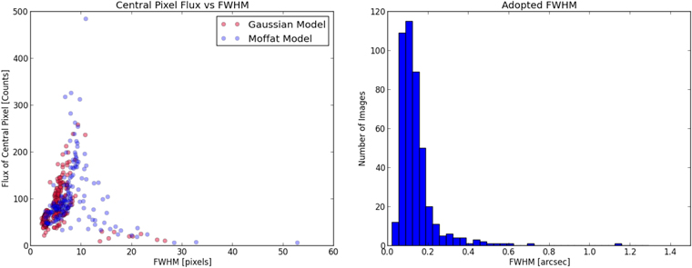
Figure 3. FWHM relation to source brightness, for both the Gaussian and the Moffat functional fits (left panel), and final adopted FWHM value as given in Table 1 (right panel).
Download figure:
Standard image High-resolution imageThe shape of the PSF varies as observing conditions and equipment performance change. It is for this reason that we combine local-in-time images to create the empirical PSFs for subtraction from individual sources (Figure 1). Consequently, the theoretical model that most effectively approximates the PSF also changes over time. For each final image set, we therefore chose whichever model (Moffat or Gaussian) produced a smaller rms residual error term for the central nine pixels, in order to define the FWHM. The mean and median FWHM values are 6.45 and 5.51 pixels or 014 and 012. For the high-FWHM, faint sources, the Moffat fit yields better results. Similarly, for the low-FWHM, bright sources, the Moffat fit also yields better results.
The FWHM values are reported in Table 1. As expected, they are anti-correlated with the contrast sensitivity limits that are presented below.
Table 1. Characteristics of Observed Targets
| Cluster | Targeta | R.A. | Decl. | V | I | J | K | Robo-AO Multiplicity | FWHMb | Robo-AO Contrast Distribution | |||
|---|---|---|---|---|---|---|---|---|---|---|---|---|---|
| 05 |
1'' | 2'' | 3'' | ||||||||||
| (degrees) | (mag) | (pix) | (Δmag) | ||||||||||
| Pleiades | AKIV 314 | 58.53719 | 24.33364 | 12.48 | 11.23 | 10.38 | 9.72 | detected binary | 9.1 | 2.92 | 4.47 | 5.96 | 6.22 |
| BPL 167 | 57.03671 | 25.02939 | 16.19 | 13.65 | 12.20 | 11.25 | single | 6.5 | 2.05 | 3.03 | 3.58 | 3.62 | |
| BPL 273 | 58.21706 | 25.17400 | 16.27 | 13.73 | 12.38 | 11.53 | likely single | 4.8 | 1.68 | 2.85 | 3.32 | 3.34 | |
| DH 027 | 53.29373 | 22.52204 | 15.55 | 13.36 | 12.12 | 11.25 | single | 6.0 | 2.06 | 3.27 | 3.81 | 3.86 | |
| DH 056 | 54.10133 | 22.62379 | 14.14 | 12.37 | 11.35 | 10.56 | detected binary | 6.5 | 1.84 | 2.99 | 3.77 | 3.90 | |
Notes.
aIn the Pleiades, our naming convention follows that of Stauffer et al. (2007) for the stars from that list. For other stars from Bouy et al. (2015), we generally chose to use the name from the first published survey that included the star as a likely Pleiades member. Names are SIMBAD-compliant if preceded by "Cl* Melotte 22," with the exception of those noted as "s," which come from the catalog of Sarro et al. (2014)—http://vizier.cfa.harvard.edu/viz-bin/VizieR?-source=J/A+A/563/A45. In Praesepe, we attempted to follow the standard convention of referring to the star by the name given to it in the first paper that ascribed cluster membership. Names are SIMBAD-compliant if preceded by "Cl* NGC 2632," with the exception of those noted as "AD," a nomenclature originating in Kraus & Hillenbrand (2007) to refer to stars first identified as Praesepe members by Adams et al. (2002). In NGC 2264, the naming convention is that of the Stauffer et al. Spitzer variability survey (https://irsa.ipac.caltech.edu/data/SPITZER/CSI2264/). Names are SIMBAD-compliant as recorded. bThe Robo-AO platescale is sampled at 21.55 mas pixel−1.Only a portion of this table is shown here to demonstrate its form and content. A machine-readable version of the full table is available.
Download table as: DataTypeset image
4. Analysis of Detected Binaries
To determine the existence of binarity, we first used the DS9 V7.3.2 software7 to examine the final image of each target. Overall brightness and contrast were varied, and contour plots were produced to identify the candidate binaries.
4.1. Astrometry
DS9 was also used to roughly gauge the relative locations of the constituent stars in a pair. For improved precision, we used the Aperture Photometry Tool (APT; Laher 2015) software8 to determine the pixel centroids of each star in the initial cutout images. APT operates via a GUI with which users may manually place an aperture on a source. APT then uses iterative methods to compute centroid positions and—as discussed in the next section—aperture fluxes (Laher et al. 2012).
Before we could calculate the binary separations and position angles, we had to correct each primary centroid for image distortion (Riddle et al. 2015). Each cutout image has a reference coordinate with respect to the earlier-stage full image taken by the Robo-AO instrument, enabling us to apply the published distortion correction. We then calculated the separation and rotation for each binary, using the corrected centroids and knowledge of array orientation relative to true north. Finally, pixel separations were converted to physical separations in au, adopting the plate scale sampling of 21.55 mas and respective distances of 136, 175, and 740 pc for the Pleiades, Praesepe, and NGC 2264 clusters.
An appropriate typical error for the measured separations is ∼002, and for the measured position angles is ∼0 1–03; the true error in the latter is dominated by an additional uncertainty in the instrument orientation, perhaps up to 15, based on repeated calibrations using globular cluster fields (Baranec et al. 2016).
4.2. Photometry
By convention, the star that is visibly brighter is designated as the primary, and its companion is the secondary. To obtain the difference in brightness between the two stars of each binary system, we used APT to measure the magnitude of each source inside an aperture, along with an uncertainty. Aperture corrections are not needed, because we are measuring relative magnitudes and the PSFs of each star are the same, given that they appear in the same image.
We used Model F for background correction within APT, which is a non-annulus-based local estimate for the sky background considering a grid size of 64 pixels and window size of 129 pixels. The other five sky subtraction models APT offers take the mean, median, or mode of a manually placed sky-annulus, set the sky value manually, or apply no sky subtraction. We decided against using any of the models that are based on a sky annulus because the target stars are very large with respect to the image size and have varying size and FWHM, so determining sky annulus radii introduced an unnecessarily arbitrary element to the analysis. For very faint secondary stars or binary systems with small separations, the algorithm used by APT to obtain centroids could not pinpoint the secondaries on the initial cutouts. In these cases, we used the PSF-subtracted remainder images to measure position centroids and magnitudes.
For each image, we explored both a constant aperture of radius of 5 pixels (011, containing about 83% of the encircled energy) and a custom aperture of radius 10–30 pixels, sufficient to cover 92%–96% of the flux, even for the poor-quality images, for each member of each binary. The magnitude difference discrepancies between the constant aperture and the custom aperture form a roughly Gaussian distribution. Our final photometry values come from the smaller aperture, in order to avoid contamination from the other member of the pair. Figure 4 illustrates the APT-reported measurement error as a function of the APT-reported instrumental magnitude.
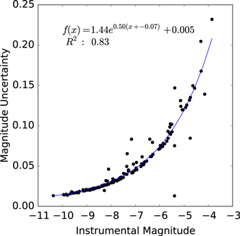
Figure 4. Photometric measurement error as a function of source brightness for the APT photometry. As expected, the uncertainties increase exponentially toward fainter magnitudes. The legend provides the fit results and corresponding coefficient of determination, which ranges between 0 and 1, where a value of 1 would indicate a perfect fit within the expected variance. High outliers represent images with higher than typical noise. Low outliers occur in cases where secondary stars were found using the PSF-subtracted image. An approximate zero point scaling is that −8 mag on the instrumental scale corresponds to roughly 12.75 mag on a Vega scale. The photometry thus spans the magnitude range ∼10.5–16.5 mag.
Download figure:
Standard image High-resolution imageFor all detected binary systems, we computed magnitude differences and associated errors. We performed an independent check of the photometry using the pipeline described in Law et al. (2014a) and Ziegler et al. (2017). For sources with close separations, the later values are preferred, given the explicit de-blending, reducing the measured contrast for these objects over straight aperture photometry. Excluding these outliers, the mean contrast difference between the two methods was 0.01 mag and the dispersion 0.14 mag, with point-to-point agreement at the <1–2 sigma level.
A significance for each companion detection was calculated using the methods employed in Ziegler et al. (2017). Briefly, the local noise as a function of separation from the target star is measured by sliding a 10 pixel diameter aperture within concentric annuli centered on the target star. The signal within the aperture at each position is measured, and the mean and standard deviation of the set of signals in each annulus is calculated. If the annulus contains an astrophysical source, the measured signals for that annulus are sigma-clipped to remove the outlier signals associated with the source. An aperture is subsequently placed on the observed nearby star, and the signal is compared to the local noise to estimate the detection significance.
Table 2 reports contrast values and a significance for each companion detection, both measured as described above.
Table 2. Basic Characteristics of Detected Binaries
| Cluster | Binary | Significance | Projected Separation | Position Angle | Optical Brightness Ratio | Mass Ratio |
|---|---|---|---|---|---|---|
| σ | (arcsec) | (degrees) | (Δmag) |
 ] ] |
||
| Pleiades | AK IV-314 | 9.7 | 1.03 | 121.2 | 2.37 ± 0.05 | 0.53 |
| DH 056 | 10.6 | 2.52 | 244.1 | 2.78 ± 0.10 | 0.33 | |
| DH 193 | 9.7 | 0.90 | 83.9 | 1.86 ± 0.08 | 0.54 | |
| DH 446 | 9.4 | 2.28 | 64.2 | 3.39 ± 0.17 | <0.23 | |
| DH 800 | 19.3 | 2.25 | 95.6 | 2.41 ± 0.05 | 0.52 | |
| DH 896 | 11.7 | 0.96 | 5.8 | 1.38 ± 0.05 | 0.57 | |
| HCG 86 | 11.1 | 1.21 | 185.2 | 0.75 ± 0.04 | 0.71 | |
| HCG 123 | 8.4 | 0.78 | 253.6 | 1.67 ± 0.06 | 0.50 | |
| HCG 354 | 6.0 | 0.45 | 179.9 | 1.21 ± 0.07 | 0.63 | |
| HCG 502 | 9.3 | 0.67 | 50.4 | 0.52 ± 0.06 | 0.82 | |
| H ii 1114 | 4.1 | 0.44 | 130.8 | 2.58 ± 0.11 | 0.40 | |
| H ii 1306 | 7.9 | 0.60 | 60.6 | 0.58 ± 0.04 | 0.87 | |
| H ii 134 | 19.1 | 1.84 | 269.4 | 0.27 ± 0.05 | 0.93 | |
| H ii 2193 | 6.0 | 0.66 | 277.8 | 2.45 ± 0.16 | 0.38 | |
| H ii 2368 | 9.7 | 0.65 | 85.4 | 2.55 ± 0.15 | 0.39 | |
| H ii 2602 | 6.1 | 0.59 | 131.4 | 0.92 ± 0.06 | 0.71 | |
| H ii 357 | 12.8 | 0.47 | 64.5 | 2.57 ± 0.11 | 0.44 | |
| H ii 659 | 15.7 | 3.42 | 233.2 | 3.15 ± 0.09 | 0.40 | |
| H ii 890 | 12.3 | 1.19 | 227.7 | 4.62 ± 0.16 | <0.18 | |
| H ii 906 | 12.3 | 1.44 | 35.4 | 2.01 ± 0.07 | 0.46 | |
| PELS 115 | 30.5 | 3.34 | 271.1 | 3.17 ± 0.07 | 0.36 | |
| s4236066 | 10.5 | 0.62 | 159.2 | 2.01 ± 0.07 | 0.41 | |
| s4337464 | 13.3 | 1.91 | 260.1 | 0.27 ± 0.05 | 0.92 | |
| s4713435 | 5.1 | 1.63 | 291.5 | 4.54 ± 0.22 | <0.17 | |
| s4955064 | 7.1 | 0.64 | 4.1 | 0.74 ± 0.05 | 0.71 | |
| s5035799 | 23.3 | 4.59 | 252.4 | 3.60 ± 0.08 | 0.20 | |
| s5197248 | 15.2 | 3.11 | 16.5 | 2.62 ± 0.06 | 0.34 | |
| s5216838 | 14.5 | 0.92 | 68.7 | 2.66 ± 0.06 | 0.41 | |
| s5305712 | 3.5 | 0.23 | 70.5 | 1.47 ± 0.03 | 0.50 | |
| SK 432 | 4.7 | 0.34 | 112.5 | 1.19 ± 0.13 | 0.57 | |
| SK 638 | 10.6 | 0.33 | 151.9 | 1.27 ± 0.16 | 0.56 | |
| SK 671 | 7.6 | 1.62 | 330.6 | 2.16 ± 0.11 | 0.44 | |
| Praesepe | AD 3085 | 12.7 | 1.22 | 86.8 | 0.48 ± 0.06 | 0.83 |
| AD 3349 | 11.9 | 2.54 | 347.3 | 3.37 ± 0.11 | 0.32 | |
| JC 10 | 10.5 | 1.38 | 266.5 | 4.55 ± 0.09 | 0.24 | |
| JS 160 | 9.4 | 0.67 | 128.8 | 2.69 ± 0.12 | 0.39 | |
| JS 19 | 6.2 | 0.33 | 295.9 | 0.98 ± 0.09 | 0.67 | |
| KW 401 | 5.5 | 1.77 | 237.6 | 3.21 ± 0.20 | 0.43 | |
| W 560 | 10.1 | 2.50 | 192.8 | 0.55 ± 0.76 | 0.86 | |
| W 889 | 15.5 | 2.04 | 63.8 | 2.39 ± 0.06 | 0.42 | |
| NGC 2264 | CSIMon-0007 | 15.2 | 1.05 | 34.5 | 1.28 ± 0.06 | ⋯ |
| CSIMon-0021 | 10.3 | 1.19 | 326.6 | 2.60 ± 0.06 | ⋯ | |
| CSIMon-0104 | 11.3 | 3.47 | 356.1 | 3.50 ± 0.15 | ⋯ | |
| CSIMon-0121 | 16.9 | 4.02 | 91.6 | 2.12 ± 0.08 | ⋯ | |
| CSIMon-0255 | 10.4 | 2.31 | 199.0 | 2.83 ± 0.09 | ⋯ | |
| CSIMon-0379 | 7.4 | 0.80 | 56.7 | 2.84 ± 0.15 | ⋯ | |
| CSIMon-0389 | 11.8 | 2.28 | 318.6 | 2.87 ± 0.16 | ⋯ | |
| CSIMon-0394 | 5.5 | 0.86 | 266.2 | 4.10 ± 0.23 | ⋯ | |
| CSIMon-0438 | 9.4 | 1.21 | 140.9 | 2.03 ± 0.11 | ⋯ | |
| CSIMon-0498 | 12.9 | 2.93 | 175.9 | 3.02 ± 0.07 | ⋯ | |
| CSIMon-0502 | 6.1 | 0.94 | 149.4 | 2.40 ± 0.12 | ⋯ | |
| CSIMon-0516 | 21.6 | 6.14 | 255.8 | 0.94 ± 0.07 | ⋯ | |
| CSIMon-0518 | 8.5 | 1.31 | 146.8 | 0.56 ± 0.04 | ⋯ | |
| CSIMon-0606 | 18.5 | 3.26 | 266.5 | 3.40 ± 0.10 | ⋯ | |
| CSIMon-0613 | 9.0 | 0.33 | 119.1 | 1.65 ± 0.12 | ⋯ | |
| CSIMon-0784 | 8.5 | 0.79 | 232.8 | 3.48 ± 0.10 | ⋯ | |
| CSIMon-0991 | 8.8 | 3.19 | 350.0 | 2.51 ± 0.16 | ⋯ | |
| CSIMon-1075 | 17.6 | 5.30 | 0.4 | 0.96 ± 0.05 | ⋯ | |
| CSIMon-1149 | 4.5 | 0.91 | 18.2 | 0.48 ± 0.14 | ⋯ | |
| CSIMon-1199 | 9.6 | 2.09 | 352.7 | 0.61 ± 0.05 | ⋯ | |
| CSIMon-1200 | 8.1 | 0.51 | 267.3 | 2.50 ± 0.11 | ⋯ | |
| CSIMon-1236 | 5.0 | 0.73 | 16.9 | 0.71 ± 0.06 | ⋯ | |
| CSIMon-1248 | 14.2 | 2.41 | 173.5 | 3.22 ± 0.08 | ⋯ | |
| CSIMon-1573 | 5.1 | 0.82 | 175.0 | 4.05 ± 0.13 | ⋯ | |
| CSIMon-1824 | 4.5 | 0.89 | 205.1 | 0.96 ± 0.05 | ⋯ | |
| CSIMon-6975 | 10.3 | 2.37 | 51.3 | 1.08 ± 0.12 | ⋯ |
5. Analysis of Images with No Detected Companions: Contrast Limits
Only a fraction of the observed sources had identifiable companions. To assess our ability to detect binary stars and determine upper limits for undetected companions, we generated contrast curves for each final image. A contrast curve denotes the separation-dependent relative brightness level a secondary star needs to exceed in order to be detected in the image. Naturally, at decreasing separations from the primary, secondary stars need to be increasingly brighter for detection to take place. An experimental contrast curve was generated by isolating the PSF of the primary and background-subtracting, then finding the median counts within a sky annulus encompassing 38–43 pixels from each centroid position. The PSF was then scaled down and placed into the original image at a series of random separation and random primary-secondary magnitude differences. The modified image was examined visually to see if the inserted secondary stars could be detected by eye, leading to rough contrast estimates of 3–6m at 05–3''.
A more sophisticated algorithm for theoretical contrast curve generation involved first converting all pixels into polar coordinates with origin at the primary star centroid. Next, we placed the maximum number of tangent circles (apertures) with a radius of five pixels around a circle describing the polar points at a given separation. For separations less than seven pixels, we used a set number of three such apertures, placed 120° apart. For each of these apertures around each circle, the enclosed flux was measured, with the fluxes of partial pixels estimated using the ratio of areas within and outside the aperture's five-pixel radius. Next, the standard deviation and the mean of all the fluxes measured at a given separation was found. The three-sigma contrast limit was generated at each separation using three times the standard deviation, added to the mean flux level at that separation. Stated as a formula, we computed the contrast at separation r to be

where Sr is the set of flux values within an annulus around r, and  . For binary stars, the procedure was modified to exclude those apertures with centers located within 30 pixels of the secondary star center.
Contrast curves were generated for every final image. Figure 5 illustrates the results for three examples of varying image quality. In Table 1, we provide the contrast values as magnitude differences at 05, 1'', 2'', and 3'' angular separation, for all sources. The tabulated contrast curve data exhibit approximately normal distributions, with means and standard deviations at the four separations of:  at 05,
  at 1'',
  at 2'', and
  at 3''.
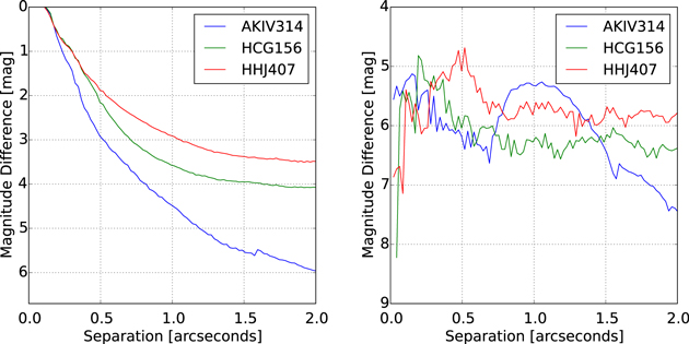
Figure 5. Contrast curves for three stars of varying image quality; raw contrast is on the left and PSF-subtracted contrast on the right. The stars illustrated are: AK IV-314, which was one of the most well-imaged stars, but is a binary system with separation of 103; the secondary has been subtracted before generating the contrast curves (resulting in the artifact discontinuity around 16). HCG-156 is representative of the mean performance, and is a single star. HHJ-407 is about one standard deviation away from the mean performance. As illustrated in the right panel, PSF subtraction improves the contrast by several magnitudes, though companion detection is still not possible below ∼02 (roughly  ). The broad bump for AK IV-314 is the residual of the seeing halo of the subtracted companion.
Download figure:
Standard image High-resolution imageIn order to further investigate the data quality, we examined the relationship between measured image FWHM and the change in the contrast values between 1'' and 05. The correlation affirms that steep contrast curves come from low-FWHM, high-quality data. Anomalously poor contrast curves have large FWHMs and are generally due to fainter sources and poor image quality.
As a check on multiplicity, the contrast curves themselves were examined for bumps that could indicate binary stars. One new binary, of no particular dimness, that was overlooked in the earlier binary identification analysis was found in this manner: CSIMon-0021.
6. Cluster Multiplicity Results
Our Robo-AO survey covered about 10% of the known cluster membership in each cluster (ranging from 8% of known NGC 2264 members to 14% of known Pleiades members). The NGC 2264 sample is comprised largely of FGK spectral types, while the Praesepe and Pleiades samples are largely K and early M types.
Figure 6 illustrates the color–magnitude diagrams for known members of the three clusters, with those detected as singles or binaries in Robo-AO data highlighted. Figure 7 shows a color–magnitude plane in which the binaries stand out from the main cluster sequences somewhat better, for a broader sample of Pleiades and Praesepe members. The morphology of the Pleiades and Praesepe plots is consistent with the roughly main-sequence nature of these clusters, while the NGC 2264 plot is both pre-main sequence and dominated by color excesses due to extinction and dust disks. The main point is that the distributions of both the Robo-AO observed stars and the detected binaries are consistent with the general distribution of objects with similar color and magnitude.
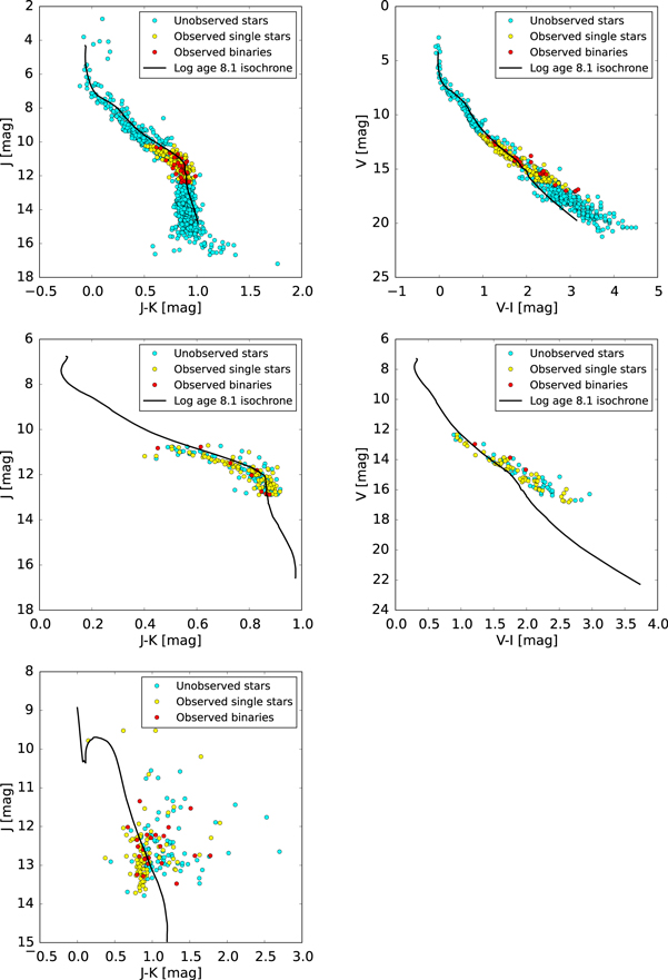
Figure 6. Color–magnitude diagrams using 2MASS (Cutri et al. 2003) near-infrared and literature optical photometry for the Pleiades (top), Praesepe (center), and NGC 2264 (bottom). Shown in each panel: unobserved cluster members for which K2 time series photometry exists (cyan), Robo-AO observed single stars (yellow), Robo-AO detected pairs (red), and a theoretical isochrone at the appropriate age, distance, and average reddening for the cluster. The Robo-AO observed samples typically span about two magnitudes in brightness within each cluster; for the Pleiades, the full color–magnitude sequence is shown for context, while just the magnitude range of relevance to Robo-AO is shown for Praesepe and NGC 2264. Clear cluster loci can be seen for Praesepe and the Pleiades, but the locus for NGC 2264 is smeared due to the combined effects of circumstellar disks and extinction.
Download figure:
Standard image High-resolution image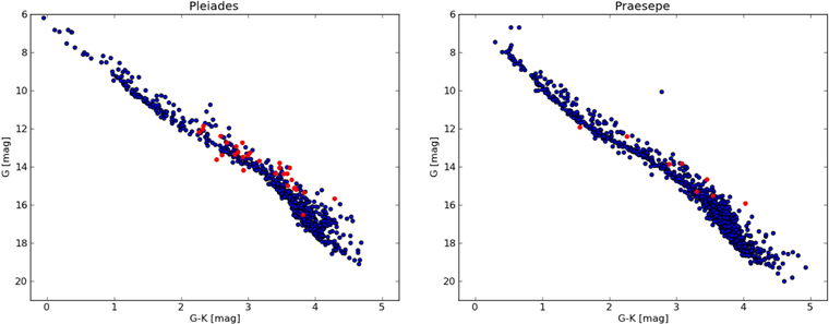
Figure 7. Location of the identified binaries (red) in an optical-infrared color–magnitude diagram, based on Gaia G-band (van Leeuwen et al. 2017) and 2MASS K-band (Cutri et al. 2003) photometry of the entire clusters. Relative to the main Pleiades and Praesepe cluster sequences, identified binary pairs stand out somewhat better in this color–magnitude diagram than in the infrared-only color–magnitude diagram of Figure 6.
Download figure:
Standard image High-resolution imageWe present a total of 66 candidate wide separation binaries −32, 8, and 26 in the Pleiades, Praesepe, and NGC 2264, respectively (see Table 2). Relative to the number of binaries indicated in Table 1, there are fewer sources listed in Table 2 because some members of pairs were found twice, as companions to each other, when imaged separately. Among the binaries, just five, two, and zero in the three respective clusters were revealed in a literature search as having their companions previously known. These confirmations (10% of our reported binary sample) provide confidence in our methods and detections overall. Furthermore, they allow the consideration of color information because the previously identified binaries had been observed at infrared wavelengths. We expect the separations to be about the same, given the large cluster distances, but our reported magnitude differences will be larger in the optical than in the infrared, due to the expected redder color of the fainter companions, relative to their primaries.
Figure 8 presents the image gallery of our Robo-AO detected binary systems. There were 78 images containing candidate binaries, with 70 unique sources—excluding repeats and poor quality images. Figure 9 illustrates the magnitude differences as a function of pair separation. Sources detected at higher contrast than the nominal limits come from better-than-average quality images or from the PSF-subtracted images; we note that this subset of high-contrast companions is located within ∼1''–15, suggesting that they are true bound companions. The median pair separation is 11, with the peak between ∼05–10, and continued decline toward a flat distribution beyond ∼2''. Beyond 4'', the data become incomplete in position angle, due to the square images. In physical units, the right panel of Figure 9 illustrates the rough segregation of companion sensitivity by distance. As NGC 2264 is further away, we were not sensitive to separations below ∼200–500 au. Meanwhile, we detected binaries in the 30–500 au range in the Pleiades and Praesepe samples, and to higher contrast levels than in NGC 2264.
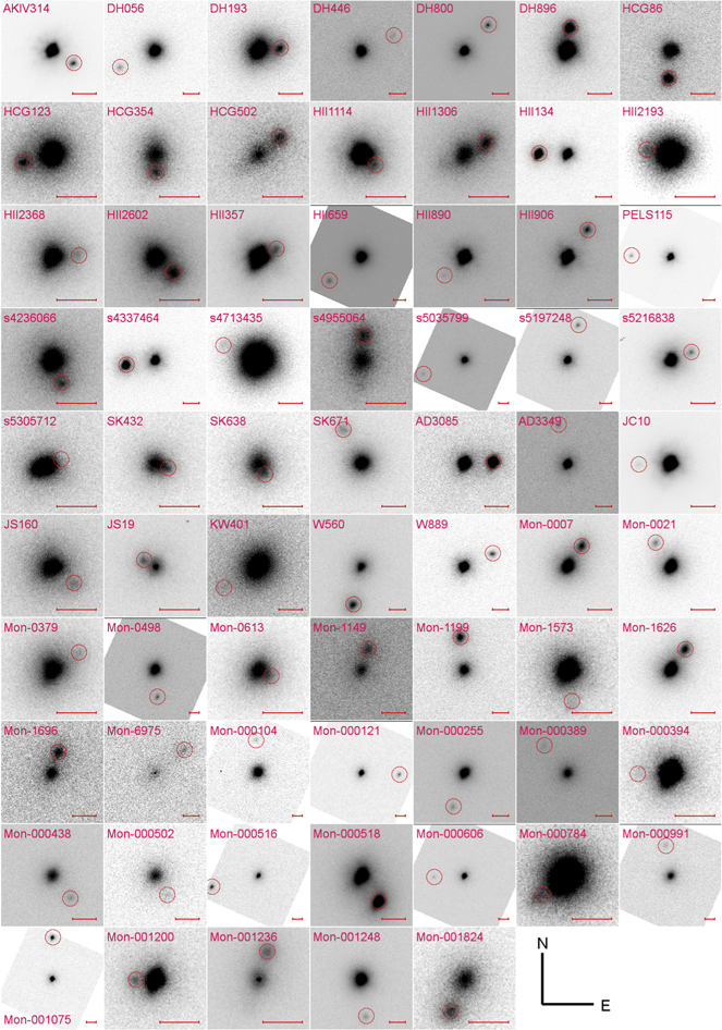
Figure 8. Robo-AO images of detected binaries; north is up and east is to the right. Red circles indicate the secondaries and red bars indicate a constant angular size of 1''. There are five different spatial scales, depending on the pair separation. Images are individually scaled in depth so as to highlight the binaries. Labels correspond to lines in Table 2, which provides the separations, position angles, differential magnitudes in the red optical, and detection significance for each system.
Download figure:
Standard image High-resolution image
Figure 9. Separation vs. difference in magnitude for detected binary systems. Members of the three clusters are individually color-coded. Left panel is in empirical units; it includes the mean  raw contrast curve and standard deviation among the contrast curves for the entire data set. PSF subtraction enables sensitivity down to 5–6 mag of contrast for most targets, as shown in Figure 5. Right panel is in physical units of au; the reduced sensitivity to small-separation companions for NGC 2264 is apparent, due to the larger distance of this cluster, as well as the lack of sensitivity for Pleiades beyond ∼585–820 au and Praesepe beyond ∼750–1050 au, on account of the maximum search radius imposed by image size. There is no correlation between separation and magnitude difference in either panel.
Download figure:
Standard image High-resolution imageNotably, there are many images on which binaries are detected at magnitude differences exceeding the individual "raw" contrast values listed in Table 1 and/or more than three standard deviations better than the nominal contrast at a given separation (left panel of Figure 5). These high contrast outliers are due to the use of PSF-subtracted images, which were generated for all final images. The PSF-subtracted data naturally have significantly better contrast, down to less than 5 mag for most targets, as illustrated in the right panel for the three examples shown in Figure 5. Five binary systems have brightness ratios of more than four magnitudes. Two of these, including the most significant outlier at the smallest separations, could not be seen in the initial image cutouts, but are clearly present in the PSF-subtracted images (and were detected in that manner). The other high-brightness-ratio systems were identified in the non-PSF-subtracted data in observations with exceptionally good contrast curves.
Results for the individual clusters are presented below. The raw multiplicity fraction across the three clusters, counting a total of 70 visual binary systems among 441 distinctly imaged targets with good Robo-AO imaging, is thus 15.9% ± 1.9% (or 15.1% ± 1.9%, if we remove duplicate pairings where each component was observed as the primary). This fraction is comparable to that of multiples found by Baranec et al. (2016) and Ziegler et al. (2017) using the same equipment but targeting a much older field star sample of comparably bright sources. However, the binary fraction varies significantly among the clusters with NGC 2264 (where we are sensitive mainly to wider separations and smaller magnitude differences, in a younger cluster) ∼50% higher, Pleiades at about the mean value, and Praesepe ∼50% lower. Because of the different cluster distances and ages, as well as the varying observing conditions during data acquisition, the sensitivity to companion separation and mass varies. Furthermore, the targets have different primary masses in NGC 2264, relative to the Pleiades and Praesepe samples, because the observations were constrained within the same apparent brightness ratio. For these reasons, the necessary—but complex and uncertain—incompleteness corrections required to turn our raw multiplicity fractions into fractions for specific a and  ranges, given the primary star m1 ranges, have not been applied.
6.1. The Pleiades at 136 pc
In the Pleiades cluster, 34 binary systems (including two pairs that were observed twice and identified as binaries of each other, thus making 32 unique pairs) were found among 212 targets.
H ii 1306, a 060 separation and  system was also identified as a binary by Richichi et al. (2012), who reported separation 065 and
  . H ii 134, a 184 separation and
  system, was also identified as a binary by Bouvier et al. (1997), who reported separation 183 and
  . Bouvier et al. (1997) also found H ii 2193, which we identify as a separation 066 and
  system; the previously reported separation was 069 and
  . Finally, for H ii 357, we report a companion with separation 047 and
  , while Bouvier et al. (1997) found separation 050 and
  .
.
For H ii 890, we report a companion at separation 119 and  , while Bouvier et al. (1997) found separation 174 and
  , declaring the secondary source a background field object. This is the only detected pair with apparent relative motion between the components, and it is also the only pair with a bluer color for the secondary relative to its primary.
A raw multiplicity of 16.0% ± 1.4% was obtained from our observations of Pleiades KM primaries.
Notes on individual sources: One of the final images, H ii 370, contained a false tripling artifact of the image acquisition, and thus could not be analyzed. One of the single stars, s4798986, was also excluded from analysis due to poor imaging. Three likely single stars, BPL 273, H ii 34, and HCG 194, were "lumpy" rather than cleanly detected as binaries. Uncertainties regarding these targets add to the uncertainty of our reported multiplicity fraction.
6.2. Praesepe at 175 pc
Out of the 108 Praesepe targets, eight were observed to be likely binaries.
As for the Pleiades, several of our optically identified Praesepe systems appear in previous literature announcing detected companions. KW 401 is reported as a 177 separation and  system, while Bouvier et al. (2001) detected KW 401 as a triple system with one component at 169 and
  at a position angle similar to our detection, and another component at separation 178 and
  that we do not see, presumably due to large optical-infrared color. We also detected W 560 as a 250 separation
  system, which Bouvier et al. (2001) report with separation 243 and
  .
.
The observed multiplicity frequency for our Praesepe sample of KM primaries is 10.2% ± 1.9%.
Notes on individual sources: One of the binary systems, JS 494, was excluded from analysis due to an additional false tripling artifact of the image acquisition. JS 231, a likely single star, and KW 566, likely a binary system, both have poor image quality and also could not be properly analyzed. Uncertainties regarding these targets add to the uncertainty of our reported multiplicity fraction.
6.3. NGC 2264 at 740 pc
Among 120 NGC 2264 targets, 34 likely binaries were detected (including eight pairs that were observed twice and identified as binaries of each other, thus making 26 unique pairs). There is no previous dedicated study of visual binaries in this cluster; a few such sources are known within the separation range to which we are sensitive (e.g., S Mon at 27 au, R Mon at 530 au, and AR6 at 2100 au), but we did not observe any of these objects. The observed multiplicity for our NGC 2264 target group of FGK primaries is 27.3% ± 4.1%.
Notes on individual sources: Images for likely binary systems CSIMon-0394, CSIMon-0890, and CSIMon-0894 were poor, and thus photometry could not be performed, so the three targets were excluded in our analysis. CSIMon-0618 and CSIMon-0486 are most likely singles, but also are of poor quality. Uncertainties regarding these targets add to the uncertainty of our reported multiplicity fraction.
6.4. Mass Ratios
The mass ratio of each identified binary system was estimated using theoretical isochrones that relate magnitude to mass. The pre-main sequence and main sequence isochrones of Siess et al. (2000) were employed in conjunction with the NextGen+AMES atmospheres of Hauschildt et al. (1999) and Allard et al. (2000) to generate V, IC, J, and Ks magnitudes. We interpolated isochrones at 125 Myr and AV = 0.15 mag, assuming a DM = 5.67, for the Pleiades; we did the same at 757 Myr and AV = 0.00 mag, assuming a DM = 6.22, for Praesepe. Due to the significant and target-dependent extinction in NGC 2264, combined with the potential influence of circumstellar disks at J and K, the mass-ratio exercise was not carried out for members of this star-forming region. Color–magnitude diagrams for the Pleiades and Praesepe clusters in J versus J − Ks, J versus J − H, and V versus V − IC demonstrate that the chosen isochrone set is a reasonable match to the cluster sequences. Generally, calculated isochrones are too blue and/or too faint for lower mass stars, especially in V versus V − Ic, compared to open cluster data; the Siess et al. (2000) models are a closer match to empirical data than most. We adopt J versus J − Ks for the mass decomposition, due to both the isochrone match and the uniform availability of data from 2MASS for our sample stars.
Previously measured magnitudes of our targets consist of the combined brightness of both stars for our identified pairs. These composite magnitudes (Table 1) were decomposed using the flux ratios tabulated in Table 2. While the flux ratios are measured in the LP600 or the SDSS i' filters, and would roughly correspond to previous measurements in the IC-band, such IC-band magnitudes are not readily available for most of the sample. Instead, the abundant J and Ks magnitudes from 2MASS were used. Furthermore, as illustrated in Figure 6, the near-infrared brightness and color predictions are better in the near-infrared than in the optical for low-mass stars. For each cluster, the point on the age-appropriate J versus J − Ks isochrone closest to each binary system was found, and then the theoretical IC magnitude corresponding to these J and Ks magnitudes was decomposed into the constituent magnitudes of the two stars. Once again using the isochrones, the corresponding mass for each magnitude was found, and a ratio was determined for primary star m1 and secondary star m2. As the isochrones did not include stars under  , only an upper limit for the mass ratio was obtained for some of the faintest secondaries.
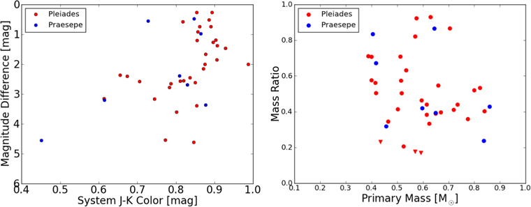
Figure 10 illustrates the mass ratios as a function of primary mass. The Robo-AO data set spans a range in  (see Table 2). Small-number statistics and the lack of incompleteness corrections prevent us from drawing any conclusions regarding the true mass ratio distribution at the wide separations probed by the data set (Figure 9).
Figure 10. Magnitude difference as a function of system composite color (left) and corresponding inferred mass ratio as a function of primary mass (right) for the Pleiades (red, with upper limits indicated by inverted triangles set by the lowest masses available from the adopted evolutionary tracks) and Praesepe (blue) binary samples. As the distributions are dominated by small-number statistics, no conclusions can be drawn beyond illustration of the range in q of the detected binaries.
Download figure:
Standard image High-resolution image
7. Discussion and Summary
Our optical multiplicity survey of 120 members of NGC 2264, 212 Pleiades members, and 108 Praesepe members covered approximately 10% of the cluster membership cataloged to date for each case. In NGC 2264, ours is the first high spatial resolution survey. In the Pleiades and Praesepe, previous similar work (notably by Bouvier et al. 1997 in the Pleiades, and by Bouvier et al. 2001 and Patience et al. 2002 in Praesepe) has been conducted at infrared wavelengths, though in sum covering a comparable number of stars to our study.
We identified 66 unique binary systems, only seven of which were previously known. Given the small contrast ratios and close separations, the majority of the newly identified companions are likely to be physically bound. Toward the low-contrast widest pairs, and the highest-contrast close pairs, boundedness becomes less likely. We can assess the likelihood of chance superposition of faint foreground or background objects using a simulation of galactic stellar populations. We queried the TRILEGAL (Girardi et al. 2005, 2012) V1.6 model9
over 1 deg2 fields toward each of the clusters, so as to establish a representative sampling of the contamination on scales of a few arcsec. The raw star counts brighter than i = 17 mag (see Figure 4) were scaled down to Robo-AO's 86 by 86 field of view, to arrive at a respective 0.0025, 0.0181, 0.0087 contaminating stars per observation toward the Pleiades, Praesepe, and NGC 2264 clusters, as expected. Multiplying by the number of sources observed in each cluster results in 0.5, 2.0, and 1.0 expected interlopers that we could be incorrectly calling binaries. However, these numbers are upper limits if one considers the smaller separations actually occupied by the observed companion distribution (see left panel of Figure 9). Specifically, we would expect only 0.08, 0.33, and 0.17 total contaminants from the three clusters at <35, where nearly all of the observed companions are located, and that any such contaminants would be close to the magnitude limit—and therefore at the higher contrast levels. Future work involving proper motions and colors is required in order to definitively establish binarity versus field star contamination.
Our observations were sensitive to only those companions located beyond the peak of the separation distribution produced by Duquennoy & Mayor (1991) and Raghavan et al. (2010) for solar neighborhood field stars. Our observations also targeted only a narrow magnitude range, which corresponds to different primary mass ranges and secondary mass sensitivities at the different cluster distances. Thus, we can not make meaningful comparisons to the features of the field star distributions in either separation or mass ratio.
Nevertheless, the results of our work broadly sample mass ratios  around primary stars with
  . The measured parameters for individual objects will be valuable for future studies aimed at placing the multiplicity results for single-age clusters in the context of field star samples with diverse ages, though better characterized multiplicity properties. Additional high spatial resolution survey work that would complete our multiplicity census for these important clusters should be carried out.
We acknowledge the Caltech SURF (Summer Undergraduate Research Fellowship) program for partially supporting the work of C. Zhang. Russ Laher provided appreciated guidance on use of the APT. Luisa Rebull provided the catalog photometry used in creating Figure 7. We thank Emma Hovanec for literature research on the targets of this study. The Robo-AO system at Palomar was supported by the collaborating partner institutions, the California Institute of Technology, the Inter-University Centre for Astronomy and Astrophysics, the National Science Foundation under grants AST-0906060 and AST-0960343, the Mount Cuba Astronomical Foundation, and by a gift from Samuel Oschin. C.B. acknowledges a Sloan Fellowship. We remain grateful to the Palomar Observatory staff for their efforts in support of astronomical research, and to the Palomar Observatory Director for the allocation of observing time to this project.
Footnotes
- 6
This is half the pixel scale quoted in Riddle et al. (2015) because the images in the present data set are oversampled by a factor of two.
- 7
- 8
- 9