


ABSTRACT
Laboratory experiments have been carried out to model the magnetic reconnection process in a solar flare with powerful lasers. Relativistic electrons with energy up to megaelectronvolts are detected along the magnetic separatrices bounding the reconnection outflow, which exhibit a kappa-like distribution with an effective temperature of ∼109 K. The acceleration of non-thermal electrons is found to be more efficient in the case with a guide magnetic field (a component of a magnetic field along the reconnection-induced electric field) than in the case without a guide field. Hardening of the spectrum at energies ≥500 keV is observed in both cases, which remarkably resembles the hardening of hard X-ray and γ-ray spectra observed in many solar flares. This supports a recent proposal that the hardening in the hard X-ray and γ-ray emissions of solar flares is due to a hardening of the source-electron spectrum. We also performed numerical simulations that help examine behaviors of electrons in the reconnection process with the electromagnetic field configurations occurring in the experiments. The trajectories of non-thermal electrons observed in the experiments were well duplicated in the simulations. Our numerical simulations generally reproduce the electron energy spectrum as well, except for the hardening of the electron spectrum. This suggests that other mechanisms such as shock or turbulence may play an important role in the production of the observed energetic electrons.
Export citation and abstract BibTeX RIS
1. INTRODUCTION
Energetic particles are ubiquitous in the universe. They show up as cosmic rays, produce synchrotron emission from distant radio galaxies, and appear in solar eruptions, like flares and coronal mass ejections (CMEs), and geomagnetic storms (Wentzel 1974). Those detected in solar eruptions are called solar energetic particles (SEPs). It is now largely accepted that there are two SEP events: impulsive and gradual (Jokipii 1966). In gradual SEP events, timing studies and the composition of SEPs suggest that these energetic particles are accelerated at a CME-driven shock with a height of several solar radii (Jokippi 1966; Reames 2013). In impulsive events, it is believed that the acceleration of electrons and ions is closely tied to the reconnection process in the flare. Various acceleration mechanisms include reconnection electric field acceleration (Litvinenko 1996), acceleration at magnetic islands (Drake et al. 2006), diffusive shock acceleration at a fast mode shock (Tsuneta & Naito 1998), and the second Fermi acceleration by turbulence (Miller et al. 1997). We note that, in many large SEP events, flares and CMEs often occur together, so it is possible that multiple acceleration processes can operate at the same time.
Magnetic reconnection is at the core of many dynamic phenomena in the universe (Adriani et al. 2009), for example, geomagnetic substorms and tokamak disruptions (Biskamp 2000; Priest & Forbes 2000). In these environments, the magnetic field may break and reconnect rapidly when twisted and sheared, converting magnetic energy into heat and kinetic energy (Yamada 2007). Because magnetic reconnection occurs in magnetic field reversals or current sheets (CSs; Petschek 1964; Sweet 1969; Thorne et al. 2005), a strong electric field is induced in the sheet, which is known as the reconnection-induced electric field (RIE field).
Part of the kinetic energy is in the energetic particles that are accelerated by the RIE field inside the CS (Figure 1). Studies of solar flares and the associated SEPs indicated that up to 10%–50% of the energy released in the flare was carried by electrons and protons with kinetic energies over 20 keV and 1 MeV, respectively, from the CS (e.g., see Lin & Hudson 1976; Aschwanden 2002; Emslie et al. 2004). In the reconnection process, the magnetic reconnection inflow brings both the magnetic field and plasma into the CS and produces the RIE field  . In the coordinate system shown in Figure 1, protons and electrons are accelerated in opposite directions by
  along the z axis, the
  ×
×  force causes them to oscillate in the y direction, and a residual magnetic field, δ
 , inside the CS, deflects them. After being turned 90° by δ
 , the accelerated particles eventually leave the CS roughly in the same direction (see Figure 1).

Figure 1. Schematic description of a CS configuration, in which  is the magnetic field outside the CS,
  is the induced electric field in the reconnection process, and δ
 is the residual magnetic field inside the CS. The trajectories of protons and electrons are described by wavy curves (from Li & Lin 2012).
Download figure:
Standard image High-resolution imageSpeiser (1965) investigated particle accelerations by the magnetic reconnection process in the geomagnetic tail for the first time. They found that the final energy of accelerated particles depends on both the electromagnetic (EM) field strength and structures in the CS. Accelerated particles would stay inside the CS forever if no residual magnetic field δ exists, and the appearance of a component of the magnetic field in the z direction (namely the guide field) helps confine the accelerated particles in the CS long enough to gain higher energy. Then Martens and Young (Martens 1988; Martens & Young 1990) noticed that a CS develops in the CME/flare configuration and suggested that what happens in the geomagnetic tail may also occur in the CME/flare CS (see also Priest & Forbes 2000).
In the above studies, the acceleration region includes a single Y-type neutral point (Y point), but the CSs in both the geomagnetic tail and the CME/flare configuration in reality are more likely to include multiple X points, among which a principal one dominates the others (Lin et al. 2005, 2008; Bárta et al. 2011; Shen et al. 2011), and the conversion of magnetic energy into the heat and kinetic energy of a plasma occurs mainly around the principal X point (see also Lin et al. 2008). Therefore, the particle acceleration in the CS including a single X point is usually considered as a local process occurring in a large-scale CS (see Li & Lin 2012; Li et al. 2013b; and references therein).
The physical properties of magnetic reconnection and the associated processes occurring inside the reconnection region have also been investigated in the laboratory for a while. Recently, high energy density laboratory astrophysics (Remington et al. 2006) has developed quickly. In this field, experiments are performed with intense lasers in the laboratory to simulate various astrophysical processes and to probe important features and key properties of these processes, allowing us to look into the physics of these processes. Extensive experiments have been performed and many works have been published within the past decade (see also Zhong et al. 2010 and Lin et al. 2015 for a brief review). Although systems in different environments possess very different scales varying over a huge range, the scaling laws (Ryutov et al. 2000) of plasma and MHD processes bring them into the same mathematical framework.
We need also to note here that extra attention must be paid when applying the scaling to the systems of interest if dissipation takes place in these systems. Ryutov et al. (2000) discussed this issue in detail. They pointed out that a large Lundquist number, Sm, is a criteria parameter for describing the astrophysical phenomena through MHD equations, and that the ideal MHD condition is a necessity for the validity of the scaling law connecting two systems of different scales in the lab and in the astrophysical environment. When studying the magnetic reconnection process, on the other hand, they further indicated that the same scaling law can also be applied if Sm is as large as 102–103.
In the magnetized plasma, the Lundquist number Sm = vAL/η, where vA is the Alfvén speed and is used as the characteristic speed, L is the characteristic length, and η is the magnetic diffusivity of the plasma in the system of interest (in the literature the expression magnetic Reynolds number ReM is also used for the Sm). Interested readers are referred to Priest & Forbes (2000, p. 35) and Priest (2014, p. 89) for more discussions. According to Remington et al. (2006) as well as Ryutov et al. (2000), the Lundquist number of the system studied in this work is given by Sm = 0.8L(cm) (eV)]2, and we follow the practice of Zhong et al. (2010) and choose Z = 13, A = 27, L = 0.1 cm, and T = 1000 eV since the arrangements for both experiments are the same. Here, Z is the charge state of the aluminum (Al) ion in the plasma appearing in our experiments, and A is the relative mass of the Al atom. This gives an Sm around 4 × 10³, which apparently exceeds 103.
Alternatively, we are also able to estimate the value of Sm on the basis of the rate of magnetic reconnection occurring in this system. As shown by Zhong et al. (2010), the experiment duplicated the main features of the two-ribbon flares, which implied that the reconnection process driven by the powerful laser beams in this kind of experiment is fast. Both analytic studies and numerical experiments have confirmed that the Sweet-Parker-type reconnection is too slow to support the energy conversion required to drive a major eruption like the two-ribbon flare. For the reconnection problem studied here, the Lundquist number for the reconnection region, SR, is related to vA, η, and the half-length of the CS Lcs as follows: SR = vALcs/η.
Consider the fact that the environment set up for our experiments is similar to that of Nilson et al. (2008), for which Fox et al. (2011) discussed properties of several important parameters. According to the discussions of Fox et al. (2011), we are able to deduce the magnetic diffusivity of the system:  m2 s−1. Zhong et al. (2010) found that vA = 4.0 × 10⁵ m s−1, and we cab measure the length of the CS,
  , from Figure 3(a) of Zhong et al. (2010). An estimate of SR on the basis of the values of these parameters gives SR = 517.
Obviously, both results for S and SR are not very different from one another for the case studied in this work and are also in the range where the scaling law connecting different systems holds. Therefore, we are allowed to use the MHD scaling law to connect the reconnection processes occurring in the solar eruption and in the laboratory to one another, and the parameters for the same physical feature in these two different systems could be well related to one another via the equations below:
where r is the characteristic length; ρ is the mass density; p is the gas pressure; v is the velocity; B is the magnetic field of the systems; and a, b, and c are transformation coefficients. The similarity of the MHD in the solar flare and in the "bench-top" flare could be seen with the transformation coefficients a = 10−11, b = 108, and c = 1010; that is, the reconnection process occurring in the laboratory could be well scaled to that occurring in the solar flare under the conditions given in (1) with coefficients of certain values. Interested readers are referred to Ryutov et al. (2000) and Zhong et al. (2010) for more details.
Laser-driven magnetic reconnection (LDMR; Li et al. 2007; Nilson et al. 2008; Zhong et al. 2010) is one of the most significant topics in laboratory astrophysics, expanding rapidly and drawing extensive attention lately. Referring to solar X-ray observations, some very similar images were also found in a recent LDMR experiment. A Faraday rotation method (Stamper & Ripin 1975) was used to measure the magnetic field in laser-produced plasmas, which can be up to a megagauss. At that time, the structure of the magnetic field was not very clear until the proton radiography technique became available (Nilson et al. 2006; Li et al. 2007, 2009). With this technique, the magnetic field that is produced in the plasma bubble by the Biermann battery effect (see Biermann 1950; Roxburgh 1966; Widrow 2002) can be measured. Such a magnetic field results from the anisotropic pressure in the plasma when a solid target is intensively irradiated by the long-pulse laser and evaporates (a nanosecond laser with intensity of around 1015 W cm−2).
The magnetic field in the universe is produced by the Biermann battery effect such that the difference in mobility between electrons and ions in an ionized plasma leads to charge separation and the breakdown of the MHD approximation. In a system filled with plasma, nonuniformities in both temperature and density occur frequently, and the gradient of the gas pressure due to the nonuniformity drives the plasma to move in the direction against the gradient, and electrons move faster than protons and the other heavy ions, resulting in an electromotive force and the associated magnetic flux. In the early universe, the magnetic field produced this way is thought to range from 10−21 to 10−19 G, which is usually known as the "seed field," and it is too weak to be detected. So the dynamo process is needed to amplify this seed field to a much higher strength, say between 10−7 and 10−5 G, which can be observed or detected (e.g., see also Widrow 2002 for more details).
In the laboratory environment, on the other hand, the Biermann effect has also been observed in laser-generated plasmas (Stamper & Ripin 1975; also see Loeb & Eliezer 1986). A plasma bubble of strong temperature and density gradients can be created as the intense laser beam irradiates a solid target, and the two gradients are nearly perpendicular, leading to a source term for the magnetic field typically megagauss in strength. In this case, the "seed" field is already strong enough to allow follow-up experiments to be performed, so the dynamo process for amplifying the magnetic field is not needed. Because the plasma in the bubble is almost fully ionized, freezing of the magnetic field to the plasma causes the field to expand together with the plasma at high speed.
Yates et al. (1982) realized the occurrence of magnetic reconnection when an unexpected X-ray emission was observed between two laser spots in a multibeam experiment. As the two bubbles expanded laterally and encountered each other with oppositely directed magnetic fields, reconnection took place, and the field lines were topologically rearranged in the diffusion region. Later, with the proton radiography technique, Nilson et al. (2006) and Li et al. (2007) diagnosed the LDMR, and some striking features were found, such as the collimated jets and magnetic null point in the diffusion region.
With long-pulse lasers, Zhong et al. (2010) constructed LDMR to model the loop-top X-ray source and outflows, which are often observed in solar flares. In their experiments, two Al foil targets were placed on the same plane, and a copper (Cu) target was placed right below the Al targets with its plane perpendicular to the Al plane (see Figure 1 of Zhong et al. 2010). Two plasma blobs were created as the Al targets were irradiated by two intense laser beams. Magnetic fields of opposite polarity associated with the plasma blobs moved toward each other as the blobs expanded, and magnetic reconnection took place between them. Two outflows were observed in the experiments. A downward outflow directly collided with the Cu target and produced a very hot X-ray spot, which was used to model the loop-top source of the X-ray emission observed in the two-ribbon flare (see Figure 2 of Zhong et al. 2010 and Figure 1 of Forbes & Acton 1996 for comparison). The flow velocity was directly measured to be 400 km s−1, which agrees well with the typical Alfvén speed in the lab environment.
Usually, the reconnection region in the laboratory environment, including the tokamak instrument, contains a single X point, but the characteristic feature of the multiple X-point reconnection, namely plasma blobs included in the CS, was also reported to appear in the lab experiments (Dong et al. 2012). Plasma blobs flowing in a CS developed by a major eruption were reported by Ko et al. (2003) for the first time and were observed in many eruptive events afterward; the numerical experiments by Forbes & Priest (1983) displayed plasma blobs in the reconnecting CS for the first time, which were then confirmed by all the subsequent numerical experiments on the related topics (e.g., see a recent review by Lin et al. 2015 for more details).
Li & Lin (2012) and Li et al. (2013b) showed that complex structures inside the CS play an important role in governing both the trajectories and spectra of energetic particles accelerated in the CS. But it is very hard, if not impossible, to observe this process directly and to perform in situ measurements for the energetic particles near the reconnection region in space, so the necessity of conducting the laboratory experiments is apparent. The importance of performing such experiments is three-fold.
First of all, it provides us a unique opportunity to investigate the particle acceleration by reconnection directly because the fundamental physics of this process throughout the universe is the same. So, the properties of possible mechanisms for cosmic-ray and even γ-ray bursts (Yuan & Zhang 2012; Meng et al. 2014), which can hardly be observed directly, might also be inferred from studying the laboratory energetic particles (LEPs) that are accelerated by magnetic reconnection.
Second, the experiments conducted here would demonstrate solid evidence that the RIE field does accelerate electrons impulsively to high energy, which is suggestive of the important role of the reconnection process in producing energetic particles in magnetically explosive events throughout the universe. And third, SEPs bring a large amount of energy from the Sun. The energy of individual particles ranges from 10 keV to 1 GeV, which can severely damage satellites and endanger astronauts in space. Therefore, studying LEPs, looking for their analogy to SEPs, and further understanding the physics behind SEPs are of great scientific and socioeconomic significance.
Following the practices of Zhong et al. (2010) and the follow-ups, we designed and performed experiments that allow us to directly detect and study the energetic particles accelerated in the LDMR process. By carefully designing the target orientation and the laser incident angle, two cases are investigated: one without a guide field, and another one with a guide field. In addition to performing the experiment itself and analyzing the consequent data, we shall also theoretically study the trajectories and energy spectra of the energetic particles produced in the CS. We do not perform particle-in-cell (PIC) simulations in this work because PIC is very computer-time-consuming; otherwise, a small proton-to-electron mass ratio, say between 100 and 200 (Drake et al. 2006), needs to be used. Perez et al. (2013) performed a PIC simulation on the related topic using the real value of the Al ion-to-electron mass ratio, and they found that it took a few times 105 CPU hours to evolve the system over a period of a few picoseconds. To save computer resources and to explore electron accelerations in the reconnection region with the correct proton-to-electron mass ratio, we use a test particle approach for our theoretical investigations. The collisionless environment where the experiment occurs (detailed arguments will be given later) also allows us to use this technique to study particle accelerations without considering particle interactions.
In next section, we introduce the setup of the experiments performed in this work; the results of these experiments and the corresponding theoretical calculations will be displayed in Section 3. These results and the physics behind them are discussed in Section 4, and finally we summarize our work in Section 5.
2. SETUP AND PERFORMANCE OF EXPERIMENTS
We perform experiments using the Shenguang II (SGII) laser facility, which can deliver a total energy of 2.0 kJ in a nanosecond (ns) square pulse. Eight SGII laser beams, at a wavelength of λL = 0.351 μm, are divided into four bunches with each bunch consisting of two laser beams. Figure 2(a) displays the arrangement of instruments used for the laser-driven reconnection experiments. Two synchronized laser bunches separated by 600 μm are focused on two aluminum (Al) foils with area of 850 μm × 500 μm and thickness of 50 μm. Each bunch is focused onto a focal spot with a diameter of 50–100 μm at the full width at half maximum, generating an incident laser intensity of ∼5 × 10¹⁵ W cm2. The two Al foils are either located in the same plane, so magnetic reconnection and the subsequent processes occur roughly in a two-dimensional (2D) configuration (case 1), or rotated oppositely away from the plane in case 1, so magnetic reconnection and the consequent phenomena of interest would occur in a 2.5D configuration (case 2), which is the case where a guide field, namely a component of the magnetic field in the direction along the RIE field, is added to a 2D configuration.

Figure 2. (a) Schematic description of the experimental setup for the laser-driven magnetic reconnection and the consequent particle acceleration studied in the present work. In this arrangement, the purple laser beams, the Al and Cu targets, and the phenomena occurring on and around them constitute the focus of this work, and the other instruments shown here are set up to measure and detect the output of the experiment. A laser beam represented by the green pipes is shot through the reconnection region for the purpose of diagnoses in the experiment. It is split into three to display the plasma structure, measure the electron density (b), and measure the Faraday rotation angle (c) and then the magnetic field in the reconnection region.
Download figure:
Standard image High-resolution imageA copper (Cu) target of 1600 μm × 250 μm area and 150 μm thickness is placed at 250 μm right below the region between the two Al foils. This Cu target plays the role of the solar chromosphere in the experiments, and a "bench-top" solar flare would be created as the downward reconnection outflow and the energetic particles accelerated by reconnection bomb it. An X-ray pinhole camera in the upper and forward direction (illustrated by the blue cone) is set to monitor the reconnection process as well as the impact of the reconnection on the Cu target. The image is taken with a 10 μm pinhole filtered with a beryllium layer of 50 μm, allowing all X-ray emission of energy above 1 keV to get through. Most of the signal from a high-energy continuum is time-integrated over 5 ns and recorded on an X-ray film that is most sensitive to X-rays in the energy range from 1 to 10 keV.
A 1000 G electron magnetic spectrometer (MS, the black box in Figure 2(a)) is located about 15 cm above the midpoint of the line connecting the centers of the two Al foils to detect the energetic electrons from the reconnection region, which covers the energy range extending to 2 MeV. The instrument distinguishes the charged particles according to their velocities. In the MS, the incident charged particles are deflected by the magnetic field. Slower particles are deflected more, and faster particles are deflected less, which eventually yields a distribution of the incident particles in space depending on their speeds on a given plane in the way particles propagate. In the instrument, an imaging plate, which is a photostimulable phosphor screen deposited on flexible plastic substrates, is placed on such a plane to collect those deflected particles, which results in the readout of the MS. Calibrating the readout to the particle energy on the basis of the known responding curves of the instrument, we are able to count the numbers of electrons of different energies.
To describe the setup of the instruments, the EM field occurring in the experiments, and both experimental and theoretical results easily and clearly, we fit the arrangement of the instruments in Figure 2 to the Cartesian coordinate system in Figure 1. This is done by performing the operations described below.
Rotating the configuration shown in Figure 1 around the z axis counterclockwise by 90° and setting the origin of the coordinate system to the midpoint of the line connecting the two Al-foil centers as displayed in Figure 2(a), we have the magnetic fields,  , shown in Figure 1 near the reconnection region aligned to those displayed in Figure 2(a). In this system, the x axis is along the line connecting the two Al-foil centers pointing rightward in Figure 2(a), the y axis points upward, and the z axis points outward from the paper.
In such a coordinate system, we realize that the direction "to observer" in Figure 1 is toward the X-ray pinhole camera and away from the shadowgraphy in Figure 2(a), and the MS was arranged such that the surface of its detector faces the origin of the coordinate system with the center of the detector surface located at the y axis. Consulting the trajectories of energetic particles (electrons and protons) leaving the acceleration region shown in Figure 1, we know that the MS is in the way of escaping accelerated electrons. In the experiments like we performed here, the charged particles that could be effectively accelerated are mainly electrons because the reconnection process is too short to accelerate protons and heavy ions because of their large inertia.
The behaviors of the plasma in the experiment are recorded by an optical diagnostic device. This device includes three channels of a 30 ps green (λL = 0.532 μm) laser beam (the so-called probe beam, represented by the green pipes in Figure 2(a)); it is employed to help collect information about the evolution in both the plasma and the magnetic field during the experiment. It is used to freeze the plasma expansion and provide a snapshot of spatial information. Through changing the delay between the probe and target beams, the expansion dynamics of the experimental plasma can be measured for all channels. As the experiment starts, the probe beam that is polarized (see Figure 2(a)) is turned on simultaneously. It first goes through the reconnection region and then is split into three: one is sent to the channel for the shadowgraphy, another one is for the Nomarski interferometer, and the third one is for measuring the Faraday rotation (refer to Figure 1 of Zhong et al. 2010 as well).
The shadowgraphy is sensitive to the secondary spatial derivative of the refractive index of the plasma, which varies with the plasma density according to the Appleton–Hartree equation (e.g., see also detailed discussions of Budden 1961 and Helliwell 2006, pp. 23–24), so it is good at displaying the contours of the plasma density in space. As the probe beam goes through the reconnection region, spatial variations in the plasma refractive index modulate the manifestation of the probe beam, and recording the modulated manifestation helps indirectly represent the inhomogeneity or structures of the plasma in space.
The Nomarski interferometer is used to measure the electron density in the reconnection region by detecting the distortion of the wavefront of the probe beam after going through that region. The distortion is also caused by the nonuniform refractive index of the plasma, which is a function of the electron density. As shown in Figure 2(b), the distorted probe beam from the reconnection region is further split by a Wollaston prism into two separate linearly polarized beams. The linear polarizer is oriented at the original polarization angle of the incident probe beam so that the two beams polarize in the same plane to guarantee that the interference between them occurs successfully. The two slit probe beams have the same amplitude, and the orientations of polarization are normal to one another. After passing through a linear polarizer, the two beams interfere and produce interfering fringes on the imaging plane of CCD. Analyzing these fringes provides us the information on the phase shift of the probe beam after going through the reconnection region, and the electron density in that region is further deduced according to the phase shift.
In addition, the third channel is just set up to measure the Faraday rotation and then the magnetic field (Figure 2(c)). The refractive index of the magnetized plasma depends on the magnetic field as well, which causes the plane where the probe wave polarizes to rotate when the wave passes through the magnetic field. This is known as the Faraday rotation and is used to measure the magnetic field in the region of interest. In our experiments, the polarization state of the incident probe beam (or wave) is known and fixed, and that of the probe wave detected at another side of the reconnection region should inevitably change because of the Faraday rotation. At this side, the probe wave including the information of the reconnection region goes through a polarized plate first, and then it is detected by a CCD (refer to Figure 2(c) for details). The initial orientation of this plate's polarization is aligned to that of the incident wave polarization, and the intensity of the probe wave behind the plate detected at this time is not necessarily at its maximum. We then continue to rotate the plate until the intensity at maximum is detected, and the Faraday rotation angle is therefore the difference between the initial orientation of the plate and that when the maximum intensity appears. This angle is linearly related to the strength of the magnetic field and the length of the path along which the probe wave propagates (e.g., see also Hutchinson 1987; Li 2000; and references therein for more details). When the instruments used in the experiment are readily arranged, the length of the path of the probe wave is thus fixed. Then with the rotation angle being measured, we are able to deduce the strength of the magnetic field.
3. RESULTS OF EXPERIMENTS AND THEORETICAL CALCULATIONS
With the setup described in the previous section, we are able to perform the experiments of interest. The typical values of plasma parameters for the environment of the experiments, such as density and temperature, are the same as those measured with interferometry and X-ray spectroscopy listed in Table 1 of Zhong et al. (2010). The hydrodynamic collision effect can also be significant during the merging of the bubbles due to the thermal pressure. Particularly if the thermal pressure is much higher than the magnetic pressure (β ≫ 1), the merging process should be dominated by hydrodynamic collision instead of reconnection, which is the case that occurred in the Omega-laser-scale merging process of a high-β experiment with β ∼ 10 and a ratio of the separation to the diameter of about unity (Li et al. 2007). Nevertheless, in the present experiments, for the onset of a driven magnetic reconnection, the laser spot separation is nearly six to seven times the laser focus diameter with a plasma beta of  (for n = 1019 cm−3, T = 1 keV, B = 106 G), which is similar to that occurring in the Vulcan experiment (Nilson et al. 2008).
By carefully designing target orientations and the laser incident angles, two cases are investigated: one without a guide field (Case 1), and one with a guide field (Case 2). In the coordinate system we have set up (see the detailed descriptions given in the previous section), our experiments in Case 1 are realized as both Al foils are located in the xy plane, and those in Case 2 are realized by rotating each Al foil 15° in opposite directions around the x axis. As described earlier, the reconnection process studied in this work takes place as a result of the interaction of two fast-expanding magnetized plasma bubbles on the Al foils. So, on one hand, if the two Al foils are arranged in the same plane, as we do for Case 1, magnetic reconnection roughly occurs in a two-dimensional fashion; on the other hand, if the two Al foils are not in the same plane, instead an angle exists between the planes where the two Al foils are located, as we arranged for in Case 2. A guide field along the z axis is hence created in the system, and magnetic reconnection happens in a 2.5-dimensional fashion (see also discussions by Zhakova et al. 2011; Li & Lin 2012; Li et al. 2013).
In Case 1, the EM field possesses the form

with a length scale of 300 μm (the half distance between two Al foil centers), a magnetic field in units of B0 = 1.2 × 10⁶ G, and an electric field in units of E0 = 3 × 10⁸ V m−1 (Nilson et al. 2008). In Case 2, on the other hand, the magnetic field generated on each Al foil contributes a cos 30° component for reconnection on the xy plane and contributes a sin 30° component for the guide field, which is a component of the magnetic field along the RIE field (Litvinenko 1996; Zharkova et al. 2011). So we have a guide field of  along the z axis in the reconnection region and two reconnecting fields of
  of opposite polarity. The E field in the z axis does not change its basic pattern as given above, but its strength decreases to
  accordingly. Therefore, the EM field becomes
in the second case with units remaining the same as those in Equation (2).
The motions of charged particles in the EM field described by Equation (2) or (3) are governed by
where m0 is the rest mass of the charged particle;  ,
,  , and
, and  =
=  /m0γ are the position, momentum, and velocity vectors of the particle, respectively;
  is the Lorentz factor with c the light speed in a vacuum; and
  is the effective collision rate (frequency):

where vTe is the thermal velocity of electrons;  with me and k being the electron mass and Boltzmann constant, respectively; and νeff is the sum of the electron collision rate, νe, and the ion collision rate, νi, namely νeff = νe + νi:

where  is the Coulomb logarithm, which is about 13 for the case we are studying here; Z = 13 is the charge state of the ion occurring in our experiments (see also Zhong et al. 2010); μ is the ion mass in units of the proton mass,
  ; ne and ni are the electron and ion density, respectively, with ne = 1019 ∼ 1020 cm−3 and ni = 1018 cm−3; and Te and Ti are the electron and ion temperatures, respectively, with Te = Ti = 1.1605 × 10⁸ K in the cases of interest (see also Zhong et al. 2010). In such an environment, we have vTe = 5.9311 × 109 cm s−1, νi = 3.4299 × 10⁵ s−1, and νe = 3.7830 × 10⁵ ∼ 106 s−1, respectively, which implies the impacts of collisions among electrons and of that between electrons and ions on the acceleration process are roughly at the same level. For simplicity, we take νe = 106 s−1 in our calculations.
The collision term in Equation (5) is due to Coulomb interactions between electrons and ions only and does not include the effect of the turbulent magnetic field in the reconnection region. The effect of the turbulent magnetic field on the motion of charged particles can be treated as "effective" collision centers. For the time being, on the other hand, the turbulent behavior of the magnetized plasma in the reconnection region is unknown; we therefore do not consider it in our theoretical calculations regarding particle accelerations, but stay with the simple motion pattern of electrons governed by the equations in (4). We understand that any discrepancy between theoretical results obtained this way and experimental ones may be due to the presence of the MHD turbulence or the shock occurring in the experiment.
As an example, we plot the local magnetic field configuration around the CS (continuous and colorful curves) for Case 2 in Figure 3, and the configuration is governed by the equations in (3). The parameters for this plot were given as before, B0 = 1.2 × 10⁶ G, E0 = 3.0 × 10⁸ V m−1, and νe = 106 s−1, and the electrons initially distribute in the acceleration region randomly (or uniformly). In this EM field, electrons are accelerated by magnetic reconnection and move in a way governed by the equations in (4). The theoretical distributions of these electrons in this region, as represented by the discrete dots around 4.3 picoseconds (ps) after reconnection commenced, are also plotted in Figure 3. As expected, most electrons in this case tend to get together around a surface of which its projection onto a plane is known as the separatrix (see below for the discussions about Figure 4). In the field of solar physics, this surface is generally known as the quasi-separatrix layer (QSL; e.g., see Janvier et al. 2015; Mandrini et al. 2015 and references therein). Since the energetic electrons play an important role in heating the lower solar atmosphere during the solar flare, the behavior of energetic electrons shown in Figure 3 helps explain why heating and flare ribbons are always observed to occur around the region where QSLs exist (see Janvier et al. 2015 and references therein).
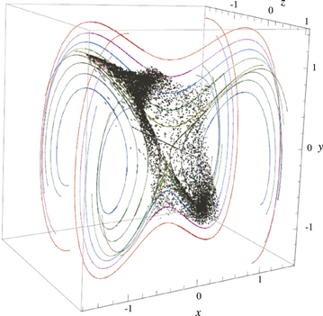
Figure 3. The magnetic configuration (continuous curves) around the reconnection region in Case 2 described by the equations in (3), and the resultant electron distribution in space around 4.3 ps after the acceleration is initiated. The motions of electrons in this region are governed by the equations in (4).
Download figure:
Standard image High-resolution image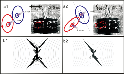
Figure 4. Comparisons of experimental and numerical simulation results. (a1)–(a2) Two laser bunches produce two plasma bubbles (in left panels) entangled by magnetic fields without (a1) and with (a2) a guide field. (b1)–(b2) Results from theoretical calculations for particle accelerations that almost duplicate the results are given in (a1) and (a2), respectively.
Download figure:
Standard image High-resolution imageThe output of experiments performed in the setup of instruments displayed in Figure 2 with the EM field described by Equations (2) and (3) is three-fold (see Figures 4 and 7). First, we obtain shadow images by the shadowgraphy, which shows the trajectories of energetic electrons that have left the reconnection region; then, the reconnection outflow and the consequence of its interaction with the Cu target are observed by a pinhole X-ray camera; and third, the energetic electrons accelerated by reconnection are collected by the MS and their energy spectra are then deduced. Among these issues, the energy and trajectories of the electrons are governed by the equations in (4), and the behavior of the reconnection outflow is governed by MHD equations that need to be solved in a different numerical approach. Since Zhong et al. (2010) already gave the relevant numerical results for a similar experiment, we do not duplicate them here but just show again some existing results to help demonstrate the effect of the guide field on the reconnection outflow. In the work below, we first discuss behaviors of the trajectory of energetic electrons and the reconnection outflows, and then we look into the energy spectra of these particles collected in our experiments.
3.1. Behaviors of Energetic Electrons and Reconnection Outflows
The laser-produced magnetic systems in the experiments are represented by the two solid ellipses in the left panels of Figures 4(a1) and (a2) for Cases 1 and 2, respectively; the gray contours in the right panels describe the trajectories of the energetic electrons accelerated by the reconnection processes occurring in the above systems consequently. They are shadow images obtained by the shadowgraphy as a probe beam passes through the region around the reconnecting magnetic structures shown in the left panels 2.5 ns after the main laser pulse peaks.
We see two major distinct beams forming a V shape ejecting from a dark area below in Figure 4(a1). Because the plasma density is high in that dark area, the probe beam is completely blocked, so the plasma situations cannot be known for this area. Instead we are using a pinhole X-ray camera to watch it. Here, we apply dashed contours in the dark region to specify the location and topology of the magnetic fields where reconnection takes place. The trajectories of energetic particles leaving the acceleration region imply that the electron is the only species that is accelerated in the experiments performed here. More discussions on this issue will be given later.
As we mentioned earlier, what happened in the magnetic configuration shown in Figure 4(a1) is a pure 2D reconnection process without a guide field. To check whether the V-shaped gray contours were of real energetic electrons accelerated by reconnection, we display in Figure 4(b1) a theoretical result for a group of electrons moving in the EM field given in Equation (2). As expected, most of the electrons in such an EM field eventually leave the acceleration region along the four separatrices of the magnetic system, constituting a region of X shape where particles accumulate. When half of this region is not visible, we see a V-shaped region. This indicates that the gray contours displayed in Figure 4(a1) were indeed the consequence of 2D magnetic reconnection.
Unlike Figure 4(a1), Figure 4(a2) displays a different scenario such that distinct major beams are ejected almost in one direction. Consulting the setup for the experiment, we know that magnetic reconnection in this case takes place in a configuration including a guide field, which is a component of the magnetic field parallel or antiparallel to the RIE field. As pointed out by Li & Lin (2012) and Li et al. (2013), the existence of the guide field in a reconnecting magnetic structure helps accelerated particles obtain more energy and changes the trajectory of the energetic particles such that electrons leave the acceleration region almost along one separatrix. Carefully studying the motions of electrons in the EM field described by the equations in (3), we end up with trajectories of these electrons as shown in Figure 4(b2), of which the continuous and zigged curves, respectively, are projections of field lines and trajectories of some of the particles displayed in Figure 3 onto the xy plane. We notice that Figure 4(b2) manifests the main features shown in Figure 4(a2).
Furthermore, looking into the details in both Figures 4(a1) and (a2), we notice that besides major beams, many minor ones randomly distributed around the major beams can also be recognized. This is very likely to imply the inhomogeneity of the reconnection process, which is similar to those observed in a CS usually developed in a real CME/flare event (e.g., see also a recent review by Lin et al. 2015). The scattering of energetic electrons by the inhomogeneous structures inside the CS may cause some electrons to leave the CS randomly (see also Li & Lin 2012 and Li et al. 2013 for more discussions), which might account for those randomly distributed minor beams in both cases.
To investigate the impact of the initial location of electrons on the distribution of accelerated electrons, we also study the acceleration of electrons that are initially distributed on the xy plane in a Gaussian fashion. The parameters for the EM field remain unchanged. Duplicating our previous calculations for Figures 3, 4(b1), and 4(b2), we obtain the distribution of energetic electrons 4.3 ps after the acceleration starts (Figure 5(a)), the trajectories of some accelerated electrons in the configuration without a guide field (Figure 5(b)), and energetic electron trajectories in the configuration with a guide field (Figure 5(c)). Comparing Figures 5(a)–(c) with Figures 3, 4(b1), and 4(b2), respectively, we can see that the basic features of both particle distributions and trajectories are the same in the two cases. This indicates that the initial distribution of electrons does not apparently affect either the distribution of accelerated electrons in the reconnection region or the trajectories as these electrons leave the acceleration region.
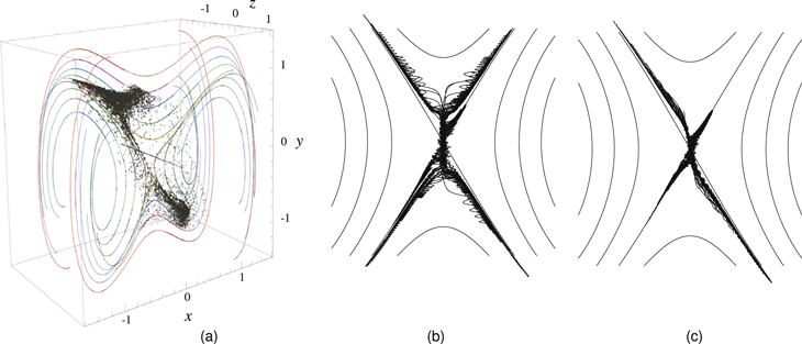
Figure 5. For the Gaussian distribution of electron initial positions on the xy plane, and about 4.3 ps after the acceleration commences, the distributions of energetic particles around the acceleration region in Case 2 (a), the trajectories of some energetic particles on the xy plane in Case 1 (b), and the trajectories of some energetic particles in Case 2 (c).
Download figure:
Standard image High-resolution imageIn addition to the energetic electrons, the associated reconnection outflows are also observed by the pinhole X-ray imaging technique, which provides images obtained forward of the Al foil targets (see Figures 6(a) and (b)). These images display the patterns of the reconnection outflows as well as the consequences of interactions of the outflow and the energetic electrons with the Cu target below, which manifests the scenario of a bench-top solar flare, a laboratory counterpart of the flare in the solar atmosphere produced by a similar process. The panels in Figures 6(a) and (b) display the interior of the reconnection region. The contours with arrows are for the magnetic structures like those in Figure 4(a) with colors for fields of different orientation. The red arrow specifies the reconnection outflow, and the black arrow indicates the X-ray emission area produced by the interaction of the reconnection outflow with the Cu target. Like energetic particles, the orientation of the reconnection outflow is apparently affected by the guide field as well.
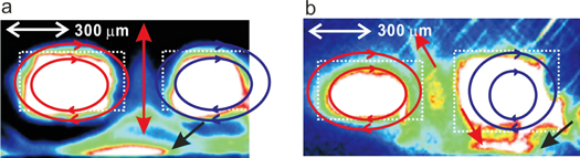
Figure 6. Patterns of the magnetic reconnection outflows in different cases. Magnetic field lines are illustrated based on the flux surface of the plasma bubbles in red and blue, respectively. In the case without the guide field (a), the outflows were ejected up- or downward normal to the surface of the Cu, and the direction of the outflow, together with the location of the "bench-top flare," changes as the guide field exists (b).
Download figure:
Standard image High-resolution imageWe further notice that the inhomogeneity in the reconnection region looks less apparent in Figure 6(a) than in Figure 6(b), which is implicitly suggestive of the role of the guide field in the formation of small structures in the reconnection region. These structures are quite likely to result from the turbulence occurring in the reconnection region. Ni et al. (2015) indicated that the turbulent features in the CS appeared more easily in the environment with a guide field than in that without a guide field, but their results showed no effect of the guide field on the direction of the reconnection outflow.
However, the effect of the guide field on the reconnection outflow seems to vary from case to case. Tharp et al. (2012) performed a systematic investigation into guide field effects on collisionless reconnection in a laboratory plasma with the the Magnetic Reconnection Experiment of the Princeton University. Their results indicated the effect of the guide field on both the rate of magnetic reconnection and the orientation of the reconnection outflow. Pritchett & Coroniti (2004) explored the physics of 3D guide-field reconnection using a PIC model in which the particle flows and magnetic flux are free to escape from the system along the magnetic field lines (see also Pritchett 2001). They found that the guide field manifested the apparent impact on the motions of ions and electrons, but almost no impact on the reconnection outflow. Frank et al. (2006) performed another set of experiments for reconnection in the laboratory similar to those by Tharp et al. (2012), but with plasmas consisting of various heavy ions: Ar, Kr, and Xe (see also Frank 1999; Bogdanov et al. 2000; and Frank & Bogdanov 2001). The reconnecting magnetic field included a singular X line and a guide field along the X line. They found that the CS became tilted and asymmetric, which differed significantly from the scenarios of magnetic reconnection taking place in the plasma with light ions, and the heavier the ions are, the more tilted the CS is. Considering the fact that the magnetic reconnection process studied in the present experiment takes place in the plasma of Al ions, which are much heavier than those of Ar, Kr, and Xe, we conclude that the difference in the reconnection outflow patterns displayed in Figures 6(a) and (b) results from a combination of the effects of heavy ions and the guide field on the magnetic reconnection process.
3.2. Spectra of Energetic Electrons
The data collected by the MS (refer to Figure 2) include information on the particle energy. Using these data, we are able to deduce the number of electrons per unit energy dN/dE at a given energy E, and plotting dN/dE versus E, as shown in Figure 7(a) for Cases 1 (black curve) and 2 (red curve), respectively, gives the differential energy spectrum of the particles. Figure 7(a) plots one set of data for each case as an example. Both curves include a thermal component at low energy (below 200 keV) and a non-thermal component at high energy (above 200 keV). This is a so-called Kappa-like distribution (see also discussions of Kasparová & Karlický 2009 and Bian et al. 2014), which is quasi-Maxwellian at the low and thermal energy band and decreases as a power law at the high and non-thermal energy band. The intersection between the thermal and non-thermal components on these curves determines an "effective temperature," which is about 109 K for the data collected in our experiments. The existence of the thermal component of energetic particles with a very high effective temperature implies the occurrence of the intense heating in the process of the particle energization.

Figure 7. Differential energy spectra of energetic electrons. The two curves in panel (a) are from the experiments. Black and red curves in all three panels are for the cases without and with a guide field in the EM field, respectively. The blue curves in panels (b) and (c) result from numerical simulations that only consider the effect of the reconnecting electric field, and the thermal electrons distribute uniformly on the xy plane prior to the acceleration (see text for more details).
Download figure:
Standard image High-resolution imageWhat is remarkable is that the spectra in both cases show an apparent hardening in the energy range of E > 500 keV, which indicates that the non-thermal part of the energy spectra of particles includes two components, a soft one and a harder one, and they join at E ≈ 500 keV. Fitting the soft one to a power-law function results in an index of around 2.5 for Case 1 and an index of around 2.6 for Case 2; fitting the harder component gives the indices of 1.5 and 1.6 for Cases 1 and 2, respectively. The occurrence of hardening at the tail of the spectrum indicates that some certain mechanisms work to enhance the particle acceleration in the reconnection region, bringing more particles to the high energy range. We discuss possible mechanisms in the next section.
Besides their similarity, the difference between these two curves is also apparent. The maximum of the dN/dE versus the curve for Case 2 shifts by 40 keV toward higher energy compared to that for Case 1. This is suggestive of an increase of the acceleration efficiency as a result of the existence of the guide field. At low energy, the two curves differ when the energy is below 70 keV. The percentage of particles with energy over 70 keV in Case 1 is about 42.0%, and it increases to 66.0% for Case 2. Theoretical investigations by Li & Lin (2012) and Li et al. (2013) indicated that the fraction of electrons accelerated from thermal energy in the solar flare region to energies higher than 20 keV is about 0.2% in the case without a guide field, and this fraction could reach up to 5% with a guide field.
With the EM field configuration occurring in the experiments given by Equation (2) or (3), together with the associated parameters, we are also able to investigate the energy spectra of energetic electrons for different cases. The initial locations of the electrons may affect the final state of the accelerated electrons, but the way they are brought into the reconnection region manifests a weak impact. The results of Li et al. (2013) indicated that the final state of the accelerated electrons does not depend on the initial locations of these electrons and the way they enter the reconnection region in the case of no guide field, and that the final state does depend on their initial locations, but not the way they enter the reconnection region, in the case with a guide field. This suggests that the guide field helps the reconnection process choose the electrons at specific initial locations to accelerate and leaves those out of these locations unaccelerated; however, the role of the guide field is not sensitive to the way the electrons enter the acceleration region. So, for simplicity, we start our calculations by assuming that all of the electrons accelerated by reconnection initially are distributed in the reconnection region randomly for both cases.
The behaviors of 5 × 10⁶ electrons in the EM field described by Equation (2) or (3) are studied. These electrons move along two separatrices and leave the acceleration region in Case 1, as shown by Figure 4(b1), or move and leave the acceleration region along one separatrix in Case 2, as shown in Figures 3 and 4(b2). In addition to the trajectory, the final energy of the accelerated electrons is another important issue that we investigate in this work. Considering the location of the MS in the setup of the instruments for our experiments (see Figure 2(a)) and following the practice of Li & Lin (2012), we count the number of electrons that leave the acceleration region along the upper separatrices as shown in Figures 4(a) and (b2), and we calculate their energies as they reach the MS. We then deduce dN/dE for these electrons according to our calculations, and we plot theoretical dN/dE versus E curves together with the experimental ones in Figures 7(b) and (c) for comparison.
When studying the impact of the electron initial distribution on motions and distributions of the accelerated electron, we have obtained the electron spectrum as well for the case that the initial distribution of electrons in the acceleration region is Gaussian. It turns out that the acceleration of electrons with the Gaussian initial distribution is slightly more efficient than that with the uniform initial distribution. Figure 8 displays the energy spectra of energetic particles in various cases for comparison. The calculations show that with a Gaussian initial distribution on the xy plane about 46.0% and 68.6% thermal electrons could be accelerated to an energy exceeding 70 keV in the EM fields without and with a guide field, respectively. Furthermore, the theoretical results are also compared with experimental ones as shown in Figure 9, which indicates that the efficiency of acceleration is slightly higher in this case than with a uniform initial distribution of thermal electrons.
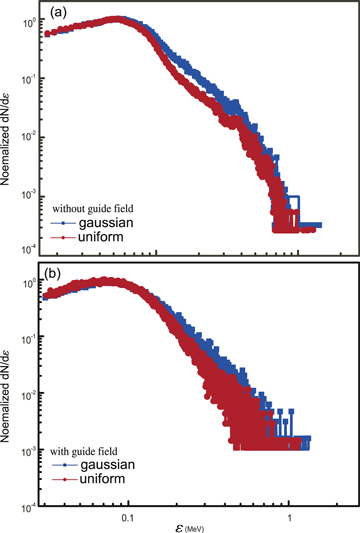
Figure 8. Differential energy spectra of energetic electrons accelerated in the EM fields not including a guide field (a) and including a guide field (b) with a uniform initial distribution (red) and a Gaussian initial distribution (blue), respectively, for comparison.
Download figure:
Standard image High-resolution image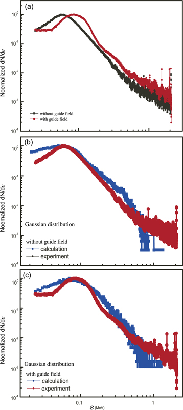
Figure 9. Same as Figure 7, but the theoretical results in panels (b) and (c) correspond to the thermal electrons distributed on the xy plane in a Gaussian fashion before the acceleration begins.
Download figure:
Standard image High-resolution image
On the other hand, although the calculated spectra in the range from 200 to 500 keV agree fairly well with the experimental ones, they fail to fit the thermal and hardening components. This suggests that in addition to the plasma being heated and charged particles accelerated by the simple RIE field in the reconnection region, and some extra processes or mechanisms may occur inside the same region as well that account for hardening of the energy spectra at the tail, which means that these processes or mechanisms should be able to further diffuse more accelerated particles to higher energies. Obviously, a simple and quasi-static EM field does not possess such a capability; the turbulence associated with inhomogeneous complex structures in the CS (Drake et al. 2006; Bárta et al. 2011; Shen et al. 2011; Lazarian & Vishniac 1999; and Lazarian et al. 2012), as shown in Figure 6(b), or perhaps shock structures as suggested by Kong et al. (2013) and Li et al. (2013a), are quite likely to exist in the reconnection region and play an important role in hardening the spectrum.
4. DISCUSSIONS
Following the practice of Zhong et al. (2010), we performed a set of LDMR experiments to look into the kinetic and dynamic properties of energetic electrons created by LDMR. These electrons were accelerated in a short time interval, and the energy spectrum of these electrons includes the thermal component, and the intersection of the thermal and non-thermal components indicates that the "effective" temperature of the acceleration region was up to ∼109 K. This simply suggests that the intensive heating of plasma and the energetic acceleration of electrons take place simultaneously in the same region. Considering the timescale of acceleration and heating, we point out that these energetic electrons were indeed accelerated by reconnection. Although the fast mode shock in the magnetized plasma can also heat plasma and accelerated charged particles simultaneously, its efficiency in heating a plasma and accelerating particles is low compared to that of the reconnection process (e.g., see also more details in Miller 1998; Reames 1998, 2013; Priest & Forbes 2000 and references therein). Considering the fact that the time interval of the LDMR process is very short (a few nanoseconds) and Al ions are much heavier than electrons, we conclude that the electron is the only species of particle that is accelerated in our experiments.
The theory about the charged particle acceleration by magnetic reconnection in the configuration including a single X point indicates that energetic electrons leave the acceleration region roughly along four separatrices in the case without a guide field (Case 1; see Figures 4(a1), (b1), and 5(b)). Our experiments confirmed this result such that the trajectories of energetic electrons constitute a V-shaped image in the shadowgraphy picture (the image of the upside-down V seen in the theoretical result cannot be seen because of the specific design of the instrument); the experiment also confirmed the theoretical result for the case with a guide field such that the energetic electron leaves the acceleration region along two specific separatrices (Case 2; see Figures 4(a2), (b2), and 5(c); again, electrons moving along one separatrix cannot be shown in the shadowgraphy picture). Interested readers are also referred to the discussions of Zharkova et al. (2011), Li & Lin (2012), and Li et al. (2013) for more details.
It is also worth noticing that the initial state of the electrons does not affect the kinetic behavior of energetic electrons in an apparent fashion. We studied in theory the distribution and trajectories of energetic electrons inside and around the acceleration region with different initial distributions of these electrons, and we found that we obtain almost the same result (comparing Figure 3 with Figure 5(a), and comparing Figures 4(b1) and (b2) with Figures 5(b) and (c), respectively). Regarding the dynamic behavior of energetic electrons, on the other hand, the initial distribution of electrons manifests some impact on the final energy of these electrons. Our results suggest that the efficiency of the acceleration starting with a Gaussian distribution of electrons is slightly higher than that of the acceleration starting with a uniform distribution (see the curves in different colors in Figures 8(a) and (b)).
Besides the fact that the theoretical results fit part of the experimental ones, we can also see that the non-thermal component of the energy spectra obtained from experiments becomes hardened at high energy (>500 keV), to which our theoretical results do not fit. This reminds us of the hardening of the continuum spectrum at high energies (usually hard X-ray and γ-ray emissions of ≥300 keV) that has often been observed in many solar flares (Suri et al. 1975; Silva et al. 2000; Share & Murphy 2006; Asai et al. 2013; Kong et al. 2013; Li et al. 2013a). Among the evidence that we have collected so far, the shape of the hard X-ray spectrum for the γ-ray flares does not much vary from flare to flare, and the spectra start to harden apparently at an energy of about 400 keV (e.g., see Yoshimori et al. 1985). Kong et al. (2013) performed a survey of 185 flares on the basis of the data obtained by the Solar Maximum Mission satellite, and they identified 23 electron-dominated events whose energy spectra displayed an apparent hardening at high energy. They found that the energy spectrum index in low energy ranges from 4.29 to 2.58, and that in high energy ranges from 2.22 to 1.56; compare them with the indices of the energy spectra of around 2.5 in low energy and 1.5 in high energy, respectively, deduced from our experiments for the energetic electrons (see Figure 7(a)).
Because the hard X-ray and γ-ray emissions observed in the solar eruption are usually believed to result from the bremsstrahlung due to the collision of energetic particles with a background plasma of density sufficiently high that the accelerated electrons are collisionally stopped in the corona (Xu et al. 2008), or due to streaming of these particles through the corona and impacting on the chromosphere (Benka & Holman 1994; Miller et al. 1997; Emslie et al. 2003), it has been speculated that such a hardening reflects an intrinsic hardening in the source-electron spectrum (Suri et al. 1975; Share & Murphy 2006; Asai et al. 2013). Our experiment, by detecting the energetic electrons directly, confirms this speculation. Explaining a hardening spectrum is not a trivial job, but a recent attempt suggested that a finite-width diffusive shock with whistler-like turbulence may harden the spectrum (Kong et al. 2013; Li et al. 2013a).
In our experiment, however, no knowledge of the turbulence spectrum (TS) and whether the conditions specified by Li et al. (2013a) could be satisfied is available. We shall not look further into the physics of hardening of a spectrum in this work, but we point out that the reconnection region is actually an assembly of structures of various scales and the associated processes (e.g., see a recent review by Lin et al. 2015), and the turbulent structures that satisfy the conditions set by Li et al. (2013a) should exist. In principle, hardening of the electron spectrum at the high-energy end results from the interactions of accelerated electrons with these structures, and understanding their behaviors will allow us to determine the TS. Therefore, unresolved questions in this work constitute two tasks for our work in the future: first, design and perform the experiments in the laboratory that allow us to explore the reconnection region so that the fine structures in the region and then the functional behaviors of the TS could be determined; second, design and perform numerical experiments of magnetic reconnection, similar to those by Bárta et al. (2011), Shen et al. (2011), and Mei et al. (2012), to figure out the properties of the TS in the reconnection region. With the TS known, we are able to study in detail the physics behind the hardening of the electron energy spectra and the continuum spectrum of hard X-rays and γ rays observed in the LDMR experiment and the solar flare.
In addition to the behavior of energetic electrons, we also paid some attention to the reconnection outflow, especially its response to the existence of a guide field. In the case without a guide field, our experiments, like those of Zhong et al. (2010), indicate that the reconnection outflow moves just along the y axis. But the direction of the outflow changes and many small structures were observed in the reconnection region as the guide field was imposed (see Figures 6(a) and (b)). Numerical and laboratory experiments have indicated that the turbulent structure appears in the reconnection region with a guide more easily than in the region without a guide field (Ni et al. 2015), and that the heavier the plasma ions are, the more apparent is the impact of the guide field on the reconnection outflow (Frank et al. 2006). Therefore, the occurrence of those small structures in the reconnection region and the change in the direction of the reconnection outflow observed can be ascribed to the impact of the guide field on the reconnection process taking place in a plasma including heavy ions (e.g., Al ions in our experiments).
5. CONCLUSIONS
A bench-top "solar flare" produced in the laboratory with high-energy lasers can simulate the loop-top X-ray emission and the outflow or jet that is due to magnetic reconnection (Zhong et al. 2010), similar to what occurs in a real solar flare. In addition, energetic particles, including electrons and ions, are also consequences of the reconnection process in the flare. Since the in situ detection of energetic particles in real flares is difficult, the bench-top "solar flare" is an ideal platform to look into the related particle acceleration processes closely. We have performed a series of experiments for this purpose with both 2D and 2.5D magnetic configurations. These are achieved by carefully setting the orientations of the targets and laser beams, which allows the reconnection to occur for two cases without or with the guide field. The main results of this work are summarized as follows:
- 1.Energetic electrons that escape from the magnetic reconnection region were detected. Their trajectories are located at the same place, colocated in space with the separatrices of the reconnecting magnetic field. Accelerated electrons move along both pairs of separatrices, extending from the X point in the case without the guide field, and they were confined to one pair of separatrix in the case with the guide field. This confirmed the theoretical results (e.g., see Pritchett & Coroniti 2004; Murphy & Sovinec 2008; Zharkova et al. 2011; Li & Lin 2012; Li et al. 2013b; and references therein).
- 2.Only electrons are accelerated in the experiment because the magnetic reconnection takes place in a short time interval and ions are too heavy to respond to the RIE field in the reconnection region.
- 3.The energy spectrum of accelerated electrons includes thermal and non-thermal components, and the intersection of the two components indicated an effective temperature up to 109 K. This implies that the energized electrons were originally from the hot plasma that was intensively heated by reconnection.
- 4.The initial positions of electrons do not apparently affect the kinetic behavior of accelerated electrons eventually, but it does affect these electrons' dynamic features such that the efficiency of acceleration is higher in the case where these accelerated electrons are initially distributed on the xy plane in a Gaussian fashion than in the case where these electrons initially have a uniform distribution on the xy plane. More studies on this issue are worth performing in the future.
- 5.The non-thermal component of the energy spectrum has the shape of a double power law, and the spectrum becomes hard in the range >500 keV. This is similar to the energy spectra observed in the hard X-ray and γ-ray emissions of many flares, which showed hardening at around or above 300 keV (e.g., see Kong et al. 2013 and references therein). For the time being, its mechanism is not completely clear. One of the possible explanations is shock formation in the reconnection region, as proposed by Li et al. (2013a). Turbulent or cascading structures may also play a similar role. This is a topic worthy of further experimental studies in the future.
- 6.The guide field also plays an apparent role in governing the formation of the fine structures in the reconnection region and the direction of the reconnection outflows. The fine (turbulent) structures are easier to form in a guide case (Figure 6(b)), as also indicated by the numerical experiments of Ni et al. (2015), and the guide field apparently changes the direction of the reconnection outflow in the environment of the plasma, including heavy ions (see also Frank et al. 2006).
Finally, we need to also note that the phenomenon we observed in the experiment is in 3D and our numerical experiments are indeed either in 2D or in 2.5D. The reason that we use 2D or 3D numerical experiments to explain the 3D phenomena is two-fold. First of all, in our experiments, magnetic reconnection occurs between the magnetic fields of opposite polarity entangling with the expanding plasma bubbles created by the laser irradiation on the Al foil. So if the two Al foils are placed on the same plane, the reconnection process is confined to happen roughly on a plane in an approximately 2D fashion. Second, the acceleration process in both the experiments and numerical calculations lasts a very short time, and the electrons move in the z direction a very short distance (about 1 mm) before leaving the acceleration region. Therefore, the region of particle motion in the z direction is actually finite in the simulation, and inside this region, the EM field in the simulation can be considered roughly consistent with that in the experiment. Thus, to the lowest order of approximation, we use a 2D or 2.5D simulation to help us understand the fundamental properties of the 3D phenomena for the time being. We should improve our numerical model in the future to better describe the experimental results and to better reveal the physics of our observations.
The authors are very much grateful to the SGII operation staff and the target preparation staff for valuable help and support. J.L. appreciates Nick Murphy for helpful discussions and suggestions. This work was supported by the 973 Program Grant 2013CBA01503, the NSFC Grants 11273033, 11205015, 11135012, 11220101002, 10821061, 11273055, and 11333007, CAS grant XDB09040202, and Beijing Nova Program Grant Z131109000413050.