


ABSTRACT
We apply a friends-of-friends algorithm to an enhanced SDSS DR12 spectroscopic catalog, including redshift from the literature to construct a catalog of 1588  compact groups of galaxies containing 5178 member galaxies and covering the redshift range 0.01 < z < 0.19. This catalog contains 18 times as many systems and reaches 3 times the depth of the similar catalog of Barton et al. We construct catalogs from both magnitude-limited and volume-limited galaxy samples. Like Barton et al. we omit the frequently applied isolation criterion in the compact group selection algorithm. Thus the groups selected by fixed projected spatial and rest-frame line-of-sight velocity separation produce a catalog of groups with a redshift-independent median size. In contrast to previous catalogs, the enhanced SDSS DR12 catalog (including galaxies with r < 14.5) includes many systems with z ≲ 0.05. The volume-limited samples are unique to this study. The compact group candidates in these samples have a median stellar mass independent of redshift. Groups with velocity dispersion ≲100
  show abundant evidence for ongoing dynamical interactions among the members. The number density of the volume-limited catalogs agrees with previous catalogs at the lowest redshifts but decreases as the redshift increases. The SDSS fiber placement constraints limit the catalog's completeness. In spite of this issue, the volume-limited catalogs provide a promising basis for detailed spatially resolved probes of the impact of galaxy–galaxy interactions within similar dense systems over a broad redshift range.
Export citation and abstract BibTeX RIS
1. INTRODUCTION
Compact groups of galaxies are the densest known systems, typically containing 3 to 10 galaxies within only a few tens of kiloparsecs. Since the discovery of Stephan's Quintet (Stephan 1877), numerous studies have identified small aggregations of galaxies. Rose (1977) and Hickson (1982) first identified well-defined samples of compact groups in the local universe. Since then many investigators have constructed compact group catalogs based on much more extensive galaxy surveys (Prandoni et al. 1994; Barton et al. 1996; Allam & Tucker 2000; Focardi & Kelm 2002; Iovino 2002; Iovino et al. 2003; Lee et al. 2004; de Carvalho et al. 2005; McConnachie et al. 2009; Díaz-Giménez et al. 2012).
Because the separation of galaxies within compact groups is comparable with their sizes, these dense systems have been laboratories for the study of the impact of galaxy–galaxy interactions using spatially resolved spectroscopy (Rubin et al. 1991; Alfaro-Cuello et al. 2015) and multi-wavelength observations (e.g., Bitsakis et al. 2010, 2011, 2014; Walker et al. 2010, 2012, 2016; Sohn et al. 2013; Alatalo et al. 2015; Fedotov et al. 2015; Zucker et al. 2016 and references therein). These groups are also associated with extended X-ray emission (Ponman et al. 1996; Fuse & Broming 2013; Desjardins et al. 2014). The low H i content of compact groups is probably a consequence of continuous tidal stripping or heating by gravitational interactions among member galaxies (Verdes-Montenegro et al. 2001; Martinez-Badenes et al. 2012). Low-redshift compact groups are intriguing targets for integral field unit (IFU) observations that examine internal kinematics along with, for example, spatially resolved strong-line star formation and metallicity diagnostics that probe the timescale of gravitational interactions (Vogt et al. 2013, 2015; Alfaro-Cuello et al. 2015).
The high frequency of obvious tidal interactions among compact group members suggests that their lifetime must be short (Barnes 1985; Diaferio et al. 1994). In principle, the galaxies should merge within a few-gigayear timescale. This timescale is comparable to the group crossing time. Nonetheless, compact groups are abundant in the nearby universe with space densities ranging from  to
to  (Mendes de Oliveira & Hickson 1991; Barton et al. 1996; Lee et al. 2004; Mendel et al. 2011; Pompei & Iovino 2012; Sohn et al. 2015).
The mere existence of compact groups at the current epoch remains a puzzle. Some previous studies propose that compact groups may persist for much longer than the apparent interactions would suggest (Governato et al. 1991; Diaferio et al. 1994; Athanassoula et al. 1997). On the other hand, Diaferio et al. (1994) suggest that the groups are replenished from the surrounding environment as galaxies merge. However, evaluation of the environments of compact groups in existing catalogs paints a confusing picture. In some catalogs 50%–76% are in surroundings (Ramella et al. 1994; Mendel et al. 2011) dense enough for replenishment; in the 2MASS compact group catalog only 27% (Díaz-Giménez & Zandivarez 2015) are in dense surroundings, making the replenishment model untenable.
Existing catalogs of compact groups contain some observational biases that may limit their usefulness for understanding the existence and evolution of these systems. The selection may introduce an artificial dependence of apparent group properties on redshift and may bias the environments of the selected systems. Barton et al. (1996) first derived a catalog of compact groups from a complete redshift survey. They use a straightforward friends-of-friends (FoF) algorithm to select group members separated by a fixed projected separation and rest-frame velocity difference. As a result of the selection, their catalog includes both nearby groups and groups in dense surroundings. They emphasize that previous criteria designed to select isolated systems actually introduce a bias against the inclusion of the nearest compact group candidates.
Here we extend the approach of Barton et al. (1996) to the sample of Sloan Digital Sky Survey (SDSS) Data Release 12 (DR12) at r < 17.77 (corresponding to the main galaxy sample of SDSS DR7). To capture nearby systems we enhance the SDSS redshift survey by including galaxies with r < 14.5. We use a similar FoF algorithm to select a sample of 1588 compact group candidates from the magnitude-limited catalog. This sample of compact group candidates is large enough to enable the construction of volume-limited subsamples. These samples are important for understanding observational biases, including the SDSS fiber-positioning constraint. These samples are also important for exploring the properties of the groups that are selected to be similar throughout the sample redshift range.
Section 2 describes the data we use including the galaxy sample with r < 14.5. We explain the FoF algorithm in Section 3. We also discuss the additional criteria applied by previous studies and lay out the ways that these criteria may affect the resulting catalog. We describe the resulting magnitude- and volume-limited catalogs and compare our catalogs with a previous large catalog (McConnachie et al. 2009) and explore the salient differences. In Section 4, we compare the properties of compact group candidates in the catalogs we derive with the properties of groups in previous samples. One important difference is that groups in previous catalogs have sizes that tend to increase with redshift, which is not seen in this study. In Section 5 we discuss the selection issues that may lead to this behavior. These selection issues also tend to eliminate nearby dense systems that are prime candidates for detailed multi-wavelength studies. In Section 6 we use the volume-limited catalogs to highlight the impact of the SDSS fiber-positioning constraints on the selection of compact group candidates from the redshift survey. We include an  , Ωm = 0.27, and
  .
.
2. THE DATA: SDSS DR12
We derive a sample of compact groups from the spectroscopic sample of SDSS DR12 (Alam et al. 2015) galaxies at r < 17.77. The DR12 includes redshifts for more than 2.4 million galaxies. The SDSS galaxy sample is incomplete for galaxies with r < 14.5 because of the saturation (Park & Hwang 2009). Fiber placement constraints also limit the completeness of catalogs of compact groups derived from the SDSS.
To reduce the incompleteness of the SDSS, we supplement the catalog with redshifts from the literature (see Hwang et al. 2010 for details). We also add redshifts from recent FAST observations at Fred Lawrence Whipple Observatory (Sohn et al. 2015). These additional data (FAST + literature) include 7796 redshifts for galaxies with r < 14.5 and 22507 for galaxies with  . The resulting sample contains 2,782,483 redshifts.
Figure 1 shows the  corrected, evolution-corrected absolute r-band magnitudes as a function of redshift. We use the K-correct software (ver 4.2) of Blanton & Roweis (2007) for k-correction shifted to z = 0.1, and applied the evolution correction given by Tegmark et al. (2004),
  (Hwang et al. 2012). The dashed line indicates the magnitude limit of the sample. We further restrict the catalog to galaxies in the redshift range 0.01 < z < 0.20. These limits remove the Virgo cluster and they avoid use of the low-density survey at the high-redshift end of the SDSS. This restricted redshift sample includes 654,066 galaxies.
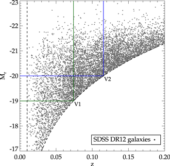
Figure 1. Absolute k-corrected r-band magnitudes of the SDSS DR12 galaxies as a function of redshift (we display only 1% of the data for clarity). Solid lines define two volume-limited samples: V1 with  and
and  mag and V2 with
  and
and  mag.
mag.
Download figure:
Standard image High-resolution imageWe adopt the morphology for compact group galaxies from the Korea Institute for Advanced Study (KIAS) DR7 value-added catalog (VAGC; Choi et al. 2010). The KIAS DR7 VAGC lists the morphology of galaxies based on the u−r color, the g−i color gradient, and on the i band concentration index (Park & Choi 2005). For the small fraction of galaxies not included in the KIAS DR7 VAGC, we visually inspect the galaxies and divide them into early and late types based on the SDSS images.
We measure stellar masses using the LePHARE4
spectral energy distribution (SED) fitting code (Arnouts et al. 1999; Ilbert et al. 2006). The mass-to-light ratio is calculated by fitting synthetic SEDs to the observed photometry. We adopt the photometric parameters of compact group galaxies from the SDSS pipeline (Stoughton et al. 2002). Synthetic SEDs are generated using the stellar population synthesis models of Bruzual & Charlot (2003). We vary the star formation history, age, extinction, and metallicity of the stellar population. The star formation histories are exponentially declining ( ) with e-folding times (τ) ranging between 0.1 and 30 Gyr. The stellar population ages range between 0 and 13 Gyr. The Calzetti et al. (2000) extinction law is adopted and E(B – V) ranges from 0 to 0.6. The models have two metallicities and we use the Chabrier (2003) initial mass function to calculate stellar mass.
3. COMPACT GROUP SELECTION
3.1. The FoF Algorithm
We use the FoF algorithm of Barton et al. (1996) to identify compact groups in the spectroscopic sample. For each galaxy, the FoF finds neighboring galaxies within a fixed projected physical spatial distance ( ) and rest-frame line-of-sight velocity linking length (
 ). The linking lengths are redshift and local density independent in contrast with some other approaches that use variable linking lengths (i.e., Huchra & Geller 1982; Tago et al. 2010; Robotham et al. 2011; Tempel et al. 2014). We use a fixed linking length here to identify systems where galaxies are separated by approximately their physical size regardless of redshift.
We bundle linked galaxies into a single galaxy system (e.g., Turner & Gott 1976; Huchra & Geller 1982; Barton et al. 1996; Tago et al. 2010; Robotham et al. 2011; Tempel et al. 2014). By construction, the resultant compact group candidates we identify have a projected physical size that is essentially redshift independent (see Section 4.1).
We test various linking lengths for the FoF. We start from a projected linking length of  and a radial linking length of
  following Barton et al. (1996) who identified compact groups from the CfA2 and SSRS redshift surveys. Barton et al. (1996) used these linking lengths because they approximately matched the median separation between Hickson compact group galaxies. Their compact groups thus have physical properties similar to the Hickson compact groups (Barton et al. 1996; Walker et al. 2016).
The linking lengths of  and
and  we choose identify 42 of the 57 Hickson compact groups. The groups we miss would require a larger linking length of
  . In general, the projected linking length of
  and the rest-frame line-of-sight velocity of
  (Barton et al. 1996) actually identify compact groups with physical sizes and galaxy number densities similar to the Hickson compact groups (see Section 4.1). Woods et al. (2010) demonstrate that these linking lengths minimize interlopers with discordant redshifts while recovering systems similar to the original Hickson compact groups. These linking lengths also have the advantage that they are often used to identify close pairs (Barton et al. 2000; Lin et al. 2004). Thus, our catalog can be combined with catalogs of close pairs in the literature and future analyses of these compact groups can be compared to previous work on pairs.
We also apply the FoF algorithm with an even tighter rest-frame line-of-sight linking length  and indicate these groups in Table 1. Previous studies of tight galaxy pairs showed that pairs with this tighter separation are more likely to be bound (Barton et al. 2000; Patton et al. 2000; Hawkins et al. 2003; De Propris et al. 2007). The subset of compact groups with this tighter radial linking length can be used for comparison with these previous galaxy pair samples.
Table 1. Catalog of MLCGs
| ID | R.A. | Decl. | nmem | za | Rgra |
 a
a
|
σa | NCb | Subsetc | V1CG | V2CG |
|---|---|---|---|---|---|---|---|---|---|---|---|
| (J2000) | (J2000) | ( kpc) kpc) |
(h3 Mpc−3) |

|
subsample | subsample | |||||
| MLCG0001 | 251.559814 | 31.722052 | 3 | 0.0534 ± 0.0005 | 30.1 ± 4.3 | 4.42 ± 0.29 | 287 ± 70 | 1 | N | ... | ... |
| MLCG0002 | 140.182175 | 33.686241 | 4 | 0.0229 ± 0.0003 | 36.8 ± 2.9 | 4.28 ± 0.13 | 170 ± 31 | 7 | S | ... | ... |
| MLCG0003 | 146.524597 | 34.623241 | 3 | 0.1318 ± 0.0010 | 20.7 ± 1.4 | 4.91 ± 0.10 | 628 ± 164 | 0 | N | ... | ... |
| MLCG0004 | 154.741531 | 37.298065 | 3 | 0.0480 ± 0.0003 | 32.9 ± 5.5 | 4.30 ± 0.42 | 210 ± 37 | 1 | S | V1CG003 | ... |
| MLCG0005 | 158.222275 | 12.086633 | 3 | 0.0330 ± 0.0004 | 12.3 ± 3.2 | 5.58 ± 0.72 | 242 ± 71 | 4 | S | V1CG004 | ... |
Notes.
aThe error is the deviation derived from 1000 time bootstrap resamplings.
bNumber of neighboring galaxies in a comoving cylinder of
deviation derived from 1000 time bootstrap resamplings.
bNumber of neighboring galaxies in a comoving cylinder of  and rest frame
  .
cDesignations for groups that contain sub-groups identified with a tighter radial linking length of
.
cDesignations for groups that contain sub-groups identified with a tighter radial linking length of  . "S" indicates a group containing sub-groups; "N" designates a group with no tighter subgroup.
Only a portion of this table is shown here to demonstrate its form and content. A machine-readable version of the full table is available.
Download table as: DataTypeset image
Hickson and others (e.g., Iovino et al. 2003; Lee et al. 2004; de Carvalho et al. 2005; McConnachie et al. 2009; Díaz-Giménez et al. 2012) apply additional criteria to define compact groups. We apply the similar population and compactness criteria applied by McConnachie et al. (2009). These criteria are a modified version of the original Hickson (1982) approach.
- 1.The population limit requires
 additional members within of the brightest group member. Here r is the SDSS extinction- and k-corrected r-band model magnitude. This criterion eliminates groups that contain one dominant galaxy surrounded by much fainter satellite galaxies.
 - 2.The compactness criterion, μr < 26 mag arcsec−2, (μr is the r-band surface brightness averaged over the group radius) excludes groups containing only low-luminosity, low surface brightness galaxies.


In the  . Here Rgr is the radius of the smallest circle encompassing all group members and Rnogal is the distance between the nearest non-member galaxy with
  and the group center. The catalogs of Barton et al. (1996) and McConnachie et al. (2009) apply a modified isolation criterion where the limiting apparent magnitude for objects in the exclusion annulus is the survey limit rather than within
  of the brightest group member.
We identify groups consisting of at least three galaxies. Hickson (1982) originally defined compact groups with at least four member galaxies, and some previous compact group surveys use his definition (McConnachie et al. 2009; Mendel et al. 2011; Díaz-Giménez et al. 2012). However, subsequent spectroscopic observations show that many of the compact group candidates selected photometrically contain only three member galaxies with accordant redshifts (Hickson et al. 1992; Pompei & Iovino 2012; Sohn et al. 2015).
3.2. Catalogs of Compact Groups from a Complete Redshift Survey
Most previous compact group catalogs have been extracted from magnitude-limited surveys (e.g., Barton et al. 1996; Iovino et al. 2003; McConnachie et al. 2009). We also construct a sample from the SDSS DR12 magnitude-limited redshift survey to obtain the largest possible sample of candidate compact groups (MLCG hereafter). In addition, we define two volume-limited samples of compact groups to explore the selection biases inherent in the magnitude-limited catalog. The two volume-limited samples include (Figure 1) galaxies with  and 0.01 < z < 0.0741 (V1) and galaxies with Mr < −20.0 and 0.01 < z < 0.1154 (V2). To construct volume-limited compact group catalogs, we apply the FoF algorithm to the two volume-limited samples independently. Table 2 lists the number of groups in each catalog and specifies the limiting survey parameters.
Table 2. The Compact Group Samples
| Sample | Magnitude Limit | z Range |
 a
a
|
 CGs CGs |
 CGs CGs |
N = 3 CGs |
|---|---|---|---|---|---|---|
| MLCGs |

|
[0.01, 0.20] | 654066 | 1588 | 312 | 1276 |
| V1CGs |

|
[0.01, 0.0741] | 149573 | 670 | 122 | 548 |
| V2CGs |

|
[0.01, 0.1154] | 210834 | 297 | 36 | 261 |
Note.
aNumber of galaxies in each sample.Download table as: ASCIITypeset image
We compare the physical properties of compact group candidates in the MLCG with previous catalogs that are also selected from magnitude-limited samples (e.g., McConnachie et al. 2009; Sohn et al. 2015). We examine some of the selection biases in the MLCG by comparing it with the two volume-limited subsets of the catalog, V1CG and V2CG (Section 6).
Fiber-positioning constraints in the SDSS introduce a systematic undersampling of regions that are dense on the sky (Strauss et al. 2002; Park & Hwang 2009; Shen et al. 2016). This undersampling leads to an incomplete catalog of compact group candidates just as it leads to an incomplete sample of close pairs. Shen et al. (2016) considered the impact of the SDSS DR6 incompleteness on samples of close pairs with separations  . They conclude that the fraction of missing pairs increases steeply with redshift for z > 0.09. Our volume-limited compact group candidate samples (Section 3.2.2) provide a measure of the bias introduced by the SDSS incompleteness. In spite of the SDSS incompleteness, the MLCG serves as a finding list, albeit incomplete, of candidate compact systems.
3.2.1. The MLCG
The MLCG contains 1588 compact groups: 312 compact groups contain  members, and 1276 group candidates contain N = 3 members. There are more N = 3 compact groups than
  compact groups at all redshifts. Figure 2 shows the distribution of the number of members in the MLCG systems. Table 1 lists the MLCG compact group candidates including ID, R.A., decl., the number of members, group redshift, group size, galaxy number density, and rest-frame line-of-sight velocity dispersion. We also note whether or not the group contains a tighter compact group satisfying the rest-frame line-of-sight linking length
  , V1CGs, and V2CGs. Table 3 lists the 5178 member galaxies contained in the compact groups of Table 1. We include the Group ID, Galaxy ID, R.A., decl., morphology, r-band extinction- and k-corrected model magnitude, u−r color, stellar mass, redshift, and its source.
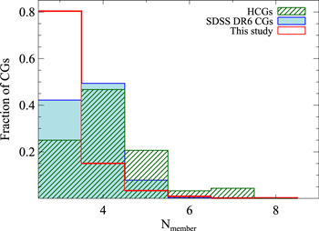
Figure 2. Population distribution of MLCG systems (open histogram) compared with Hickson compact groups (hatched histogram) and SDSS DR6 compact groups (filled histogram).
Download figure:
Standard image High-resolution imageTable 3. Catalog of MLCG Members
| Group ID | Galaxy IDa | R.A. | Decl. | Morph.b | rc | u − rc | z |

|
z Sourced |
|---|---|---|---|---|---|---|---|---|---|
| MLCG0001 | 1237661387083284633 | 251.569153 | 31.726006 | 1 | 15.02 | 2.82 | 0.0541 ± 0.00002 |

|
SDSS |
| MLCG0001 | 1237661387083284634 | 251.560486 | 31.725866 | 2 | 15.82 | 2.78 | 0.0522 ± 0.00002 |

|
SDSS |
| MLCG0001 | 1237661387083284893 | 251.549835 | 31.714281 | 1 | 17.47 | 2.58 | 0.0538 ± 0.00003 |

|
SDSS |
| MLCG0002 | 1237661383844036794 | 140.154343 | 33.706100 | 1 | 16.62 | 2.10 | 0.0224 ± 0.00002 |

|
SDSS |
| MLCG0002 | 1237661383844102154 | 140.191086 | 33.704514 | 1 | 14.73 | 3.79 | 0.0231 ± 0.00001 |

|
SDSS |
| MLCG0002 | 1237661383844102157 | 140.200195 | 33.679672 | 1 | 16.65 | 2.45 | 0.0224 ± 0.00001 |

|
SDSS |
| MLCG0002 | 1237661383844037025 | 140.183090 | 33.654678 | 2 | 17.73 | 1.73 | 0.0236 ± 0.00001 |

|
SDSS |
Notes.
aSDSS DR12 object ID. bGalaxy morphology. 1 indicates early types and 2 indicates late types. cThe SDSS extinction- and k-corrected model magnitudes. dSource of the galaxy redshift.Only a portion of this table is shown here to demonstrate its form and content. A machine-readable version of the full table is available.
Download table as: DataTypeset image
We also examine the morphological composition of the compact groups (Table 4). The fraction of early-type galaxies in the MLCG is 64.0 ± 0.01%, exceeding the fraction in the Hickson compact groups (i.e., 51 ± 2%, Hickson et al. 1988). The early-type fraction for  compact groups (69.8 ± 0.01%) exceeds the fraction for N = 3 compact groups (62.0 ± 0.01%). The error in the fraction of early-type galaxies is the
  deviation from 1000 bootstrap resamplings.
Table 4. Morphological Composition
| Catalog | CG Type | Ngalaxy | Early Types | Late Types |
|---|---|---|---|---|
| MLCGs | Total | 5178 | 3316 (64.0 ± 0.01%) | 1862 (36.0 ± 0.01%) |

|
1350 | 943 (69.8 ± 0.01%) | 407 (30.2 ± 0.03%) | |
| N = 3 | 3828 | 2373 (62.0 ± 0.01%) | 1455 (38.0 ± 0.01%) | |
| V1CGs | Total | 2175 | 1493 (68.6 ± 0.01%) | 682 (31.4 ± 0.01%) |

|
531 | 405 (76.3 ± 0.02%) | 126 (23.7 ± 0.02%) | |
| N = 3 | 1644 | 1088 (66.2 ± 0.01%) | 556 (33.8 ± 0.01%) | |
| V2CGs | Total | 930 | 704 (75.7 ± 0.01%) | 226 (24.3 ± 0.01%) |

|
147 | 127 (86.4 ± 0.03%) | 20 (13.6 ± 0.03%) | |
| N = 3 | 783 | 577 (73.7 ± 0.02%) | 206 (26.3 ± 0.02%) |
Download table as: ASCIITypeset image
Figure 3 shows the velocity dispersion of the MLCG compact groups as a function of redshift in the range 0.01 < z < 0.19. We calculate the rest-frame line-of-sight velocity dispersion of each compact groups, σCG, from Equation (1) of Danese et al. (1980). As expected, the average velocity dispersion of  compact group is generally larger than for N = 3 compact groups.
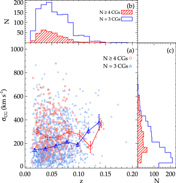
Figure 3. (a) Compact group velocity dispersion as a function of redshift. Open circles denote  compact groups; triangles denote N = 3 compact groups. Larger symbols represent the median velocity dispersion of MLCG systems in redshift bins
  . (b) Redshift distribution of compact groups for
  (hatched) and N = 3 (open) compact groups. (c) Histograms of the velocity dispersion of MLCG systems. The definitions of the histograms are the same as for panel (b).
Download figure:
Standard image High-resolution imageThere are 256 compact groups with very large velocity dispersion  , overlapping the distribution for galaxy clusters (∼400–1300
  , Rines et al. 2013). Compact group candidates with large σCG also appear in other catalogs (e.g., Barton et al. 1996; Pompei & Iovino 2012; Sohn et al. 2015). To examine the possibility that these higher velocity dispersion groups are merely superpositions along the line-of-sight, we compare the velocity dispersion distribution of the MLCG systems with the distribution for a set of ∼3000 randomly selected triplets and quadruplets in the same redshift and apparent magnitude range. To construct these random superpositions, we first pick a galaxy at a randomly chosen MLCG redshift and then randomly select two or three other galaxies within
  without attention to the projected spatial separation. The velocity dispersion distribution of these random samples is broad with
  with a median value of
  , a factor of three larger than for the MLCG objects. Figure 4 shows the probability distribution of the MLCG velocity dispersions (red) along with the distributions for the fictitious groups randomly selected from the survey redshift distribution. The distribution for the fictitious distribution (black) is appropriately weighted for the N = 3 and
  samples. Both the Kolmogorov–Shmirnov and the Anderson–Darling k-sample tests reject the hypothesis that these distributions are derived from the same parent distribution (p = 0). The overlap of the two distributions suggest that MLCG systems with
  may often contain superpositions. Furthermore, we can estimate an upper limit on the fraction of MLCG systems with
  that may be contaminated by interlopers by computing the integral of the product of the distributions in the region of overlap. The limit is about 18%. Obviously the probability that a candidate compact group includes a superposition increases as the velocity dispersion increases.

Figure 4. Probability distribution function for σCG (hatched histograms) and σlos (open histograms).
Download figure:
Standard image High-resolution imageFigure 5 shows the total observed stellar masses of the compact groups in the MLCG as a function of redshift. The stellar masses range from  , similar to compact groups in the SDSS DR6 (Coenda et al. 2015). The median observed total stellar mass of the MLCG systems increases as the group redshift increases. This dependence results from the nature of the parent magnitude-limited sample.

Figure 5. Observed stellar mass of MLCG systems as a function of redshift (small points) and their median in redshift bins. The median of observed group stellar mass among the V1CGs (diamonds) and the V2CGs (triangles) can be compared directly at different redshifts because they require no relative correction for the unobserved end of the stellar mass function.
Download figure:
Standard image High-resolution image3.2.2. Volume-limited Subsamples of the MLCG
Volume-limited subsamples have the advantage that the physical properties of the candidate systems should be the same throughout the volume. Each volume-limited sample also contains systems with a narrow range of total stellar mass. The two volume-limited samples we select highlight compact systems with stellar masses in the ranges:  (V1CG) and
  (V2CG).
The sample V1CG contains 670 groups in the redshift range 0.01 < z < 0.075 (Table 5). These groups are similar to the median groups in the MLCG for the redshift range 0.06 < z < 0.08. In contrast with the MLCG systems (red points in Figure 5), the median stellar mass for the V1CG groups is essentially constant throughout the sample redshift range. In Table 1 we indicate the MLCG groups that are also contained in the V1CG.
Table 5. Catalog of V1CGs
| IDa | R.A. | Decl. | nmem | zb | Rgrb |
 b
b
|
σb | NCc |
|---|---|---|---|---|---|---|---|---|
| (J2000) | (J2000) | ( kpc) kpc) |
(h3 Mpc−3) | ( ) ) |
||||
| V1CG001 | 198.227173 | 1.012775 | 3 | 0.0723 ± 0.0008 | 37.8 ± 5.4 | 4.12 ± 0.32 | 482 ± 116 | 8 |
| V1CG002 | 139.935760 | 33.744308 | 3 | 0.0202 ± 0.0012 | 13.0 ± 1.5 | 5.52 ± 0.19 | 866 ± 207 | 2 |
| V1CG003 | 154.741531 | 37.298065 | 3 | 0.0480 ± 0.0003 | 32.9 ± 5.5 | 4.30 ± 0.41 | 210 ± 37 | 1 |
| V1CG004 | 158.222275 | 12.086633 | 3 | 0.0330 ± 0.0004 | 12.3 ± 3.0 | 5.58 ± 0.68 | 242 ± 68 | 5 |
| V1CG005 | 127.709404 | 28.573534 | 3 | 0.0657 ± 0.0000 | 31.2 ± 3.7 | 4.37 ± 0.25 | 26 ± 4 | 1 |
Notes.
aMember galaxies are contained in the MLCG galaxy catalog (Table 3). bThe error is the deviation derived from 1000-times bootstrap resamplings.
cThe number of neighboring galaxies in the comoving cylinder.
deviation derived from 1000-times bootstrap resamplings.
cThe number of neighboring galaxies in the comoving cylinder.
Only a portion of this table is shown here to demonstrate its form and content. A machine-readable version of the full table is available.
Download table as: DataTypeset image
V2CG contains 297 groups in the redshift range 0.01 < z < 0.116 with larger total stellar masses (Table 6). For z ≲ 0.02 the median total stellar mass drops because the survey volume is too small to contain many of the most massive objects. For  , the median total stellar mass of the systems is approximately constant throughout the redshift range. The median matches the median for the MLCG for redshifts greater than z > 0.09. The V2CG systems are a subset of both the V1CG systems and the MLCG systems. Table 1 indicates group membership in these subsamples.
Table 6. Catalog of V2CGs
| IDa | R.A. | Decl. | nmem | zb | Rgrb |
 b
b
|
σb | NCc |
|---|---|---|---|---|---|---|---|---|
| (J2000) | (J2000) | ( kpc) kpc) |
(h3 Mpc−3) | ( ) ) |
||||
| V2CG001 | 154.930054 | 37.472149 | 3 | 0.0933 ± 0.0002 | 35.7 ± 1.8 | 4.20 ± 0.09 | 144 ± 35 | 1 |
| V2CG002 | 142.154663 | 36.477848 | 3 | 0.0862 ± 0.0003 | 35.8 ± 4.9 | 4.19 ± 0.36 | 183 ± 42 | 0 |
| V2CG003 | 206.682205 | 45.697647 | 4 | 0.0648 ± 0.0002 | 34.6 ± 2.9 | 4.36 ± 0.13 | 128 ± 30 | 8 |
| V2CG004 | 210.859863 | 41.869808 | 3 | 0.1130 ± 0.0001 | 40.8 ± 4.5 | 4.02 ± 0.22 | 73 ± 17 | 0 |
| V2CG005 | 179.164658 | 11.389394 | 3 | 0.0682 ± 0.0005 | 33.2 ± 5.2 | 4.29 ± 0.33 | 357 ± 113 | 5 |
Notes.
aMember galaxies are contained in the MLCG galaxy catalog (Table 3). bThe error is the deviation derived from 1000 time bootstrap resamplings.
cThe number of neighboring galaxies in the comoving cylinder.
deviation derived from 1000 time bootstrap resamplings.
cThe number of neighboring galaxies in the comoving cylinder.
Only a portion of this table is shown here to demonstrate its form and content. A machine-readable version of the full table is available.
Download table as: DataTypeset image
In Section 6 we use the V1CG and V2CG subsets of the MLCG to examine the properties of compact group candidates of the same stellar mass as a function of redshift. We also discuss the use of these samples as a basis for discussing the impact of the SDSS fiber-positioning constraints on the identification of compact group candidates.
3.3. Comparison of the MLCG with Photometrically Selected Samples
The SDSS DR6 compact group candidate sample of McConnachie et al. (2009) is the largest catalog previously available; it includes 2297 compact group candidates drawn from a magnitude-limited sample with  (catalog A) and 74,791 compact group candidates from a magnitude-limited sample with
  (catalog B). McConnachie et al. (2009) identified these compact group candidates by applying all of Hickson's criteria to the SDSS DR6 photometric galaxy sample.
Because the primary identification of the McConnachie et al. (2009) groups is photometric, the interloper fraction is substantial. By measuring additional redshifts, Sohn et al. (2015) estimate that the fraction is greater than 40%. Mendel et al. (2011) pruned the McConnachie et al. (2009) catalog by using photometric redshifts. However, the uncertainty in photometric redshifts (median  ) is large compared with the typical velocity separation among candidate group member galaxies. In spite of these limitations, the McConnachie et al. (2009) SDSS DR6 compact group candidate sample provides a basis for comparison with the MLCG. The comparison tests the impact of different group selection methods.
We match the MLCG compact groups with group candidates in catalogs A and B of McConnachie et al. (2009) based on angular separation. We count the number of MLCG systems matched (Dsep < Rgr) with group candidates in either catalog, where Dsep is the angular separation between the MLCG system and a McConnachie et al. (2009) group candidate, and Rgr is the angular radius of the MLCG. Only 242 (15%) of the MLCG systems overlap with compact group candidates identified by McConnachie et al. (2009). This low matching rate results primarily from (1) the MLCG inclusion of galaxies with r < 14.5 and from (2) differences in the group identification algorithm.
We next examine the reasons that individual MLCG systems are missing from the McConnachie et al. (2009) catalog in more detail. First, there are 384 (24%) groups in the MLCG that contain bright (r < 14.5) member galaxies excluded from the input galaxy catalog. Most of these groups are located at z < 0.05 where McConnachie et al. (2009) identified only a few compact group candidates (Sohn et al. 2015). Second, 1228 (77%) MLCG systems do not satisfy the isolation criterion originally applied by Hickson (1982) and followed by McConnachie et al. (2009). These groups have one or more non-member galaxies ( mag) within the isolation annulus (
 ), where RGCD is the groupcentric distance and Rgr is the projected group radius (see Section 5.1 for further discussion). Third, 311 (20%) triplets in the MLCG satisfy all of the McConnachie et al. (2009) group candidate selection criteria except that there are only three members with accordant redshifts. The total number of compact groups that violate each of the selection criteria of McConnachie et al. (2009) exceeds the total number of MLCG systems because some MLCG groups violate more than one criterion.
Figure 6 shows examples of MLCG systems absent from previous catalogs. These groups either contain bright members with r < 14.5 or they violate the isolation criterion. The member galaxies show active interacting features, indicating that they are physically bound systems rather than superpositions of galaxies along the line of sight. These examples underscore the impact of deriving a compact group catalog from a complete redshift survey.
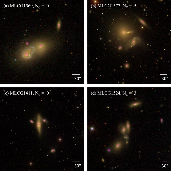
Figure 6. Sample images of MLCG systems absent from previous compact group catalogs. All these candidates violate the isolation criterion. Furthermore, (a) MLCG1569, (b) MLCG1577, and (c) MLCG1411 are missing because they contain a bright galaxy (r < 14.5). Note the striking evidence for tidal interactions in all four systems.
Download figure:
Standard image High-resolution image4. COMPACT GROUP PROPERTIES
4.1. Comparison with Other Compact Groups
We compare the physical properties of the MLCG systems with the Hickson compact groups (Hickson et al. 1992) and with the SDSS DR6 compact groups (McConnachie et al. 2009; Sohn et al. 2015). The SDSS DR6 compact groups we consider (SDSS DR6 compact groups hereafter) have spectroscopic redshifts from our FLWO/FAST observations and the literature, including SDSS DR12 (Sohn et al. 2015). The identification of these systems was adapted from Hickson's criteria (catalog A of McConnachie et al. 2009). Thus, this comparison provides a measure of the way apparent compact group properties might depend on the selection method.
Figure 7 compares the distributions of physical properties of the compact groups including redshift, velocity dispersion, projected group radius, and number density. The redshift range of the MLCG systems, 0.01 < z < 0.19, covers the range for the Hickson compact groups, but differs from the range for the SDSS DR6 compact groups (0.03 < z < 0.20 with a median z ∼ 0.08). Because we include bright galaxies and because we do not apply an isolation criterion, we find more compact groups at z < 0.03 (See Section 5.1). We miss compact group candidates at z > 0.09 because of the SDSS incompleteness (see Section 3.2) and magnitude limit.

Figure 7. Properties of MLCG systems including (a) redshift, (b) velocity dispersion, (c) projected group radius, and (d) the galaxy number density compared with other compact group catalogs. The color and fill of the histograms are the same as in Figure 2.
Download figure:
Standard image High-resolution imageThe MLCG systems have rest-frame velocity dispersions σCG  with a median of
  , similar to that for other samples. For example, the median velocity dispersions are
  for the Hickson compact groups, and
  for the SDSS DR6 compact groups. The similar selection limit for the radial separation between member galaxies (i.e.,
  ) essentially dictates that the velocity dispersion of the samples be similar.
The projected sizes of the MLCG systems differ from those of groups in other catalogs. The MLCG systems have Rgr ranging from 4 to  . The median Rgr =
  kpc is similar to that for the Hickson compact groups,
  . However, the median size of the SDSS DR6 compact groups,
  , is much larger than that for the MLCG systems or for the Hickson compact groups (McConnachie et al. 2009; Sohn et al. 2015).
Because the SDSS DR6 compact groups are apparently larger than the compact groups identified in other catalogs, the resulting galaxy number density appears to be smaller. The galaxy number density is
where N is the number of members and Rgr is the projected group radius in  Mpc. The median galaxy number density of the MLCG systems is
 ![$\mathrm{log}(\rho /[{h}^{-3}\,{{\rm{Mpc}}}^{3}])=4.36\pm 0.01$](https://content.cld.iop.org/journals/0067-0049/225/2/23/revision1/apjsaa2dabieqn100.gif) . The median is
. The median is ![$\mathrm{log}(\rho /[{h}^{-3}\,{{\rm{Mpc}}}^{3}])=4.27\pm 0.09$](https://content.cld.iop.org/journals/0067-0049/225/2/23/revision1/apjsaa2dabieqn101.gif) for the Hickson compact groups and
for the Hickson compact groups and ![$\mathrm{log}(\rho /[{h}^{-3}\,{{\rm{Mpc}}}^{3}])=3.65\pm 0.04$](https://content.cld.iop.org/journals/0067-0049/225/2/23/revision1/apjsaa2dabieqn102.gif) for the SDSS DR6 compact groups. In other words, the number density of the MLCG systems is similar to that of the Hickson compact groups, but higher than that of the SDSS DR6 compact groups (bottom right panel of Figure 7).
for the SDSS DR6 compact groups. In other words, the number density of the MLCG systems is similar to that of the Hickson compact groups, but higher than that of the SDSS DR6 compact groups (bottom right panel of Figure 7).
In principle, over the redshift range we explore here, the physical properties of the compact group candidates identified by an algorithm should not depend strongly on redshift. In Figure 8, we compare properties of the catalogs as a function of redshift beginning with the Rgr. The median Rgr of the MLCG systems varies little with redshift; in contrast, the sizes of compact groups in the catalog from McConnachie et al. (2009) and its subsamples (Mendel et al. 2011; Sohn et al. 2015) increase significantly with redshift. One possibility is that Sohn et al. (2015) selected larger groups for their follow-up redshift measurements. However, the median Rgr of compact group candidates based on photometric redshifts (Mendel et al. 2011) shows a similar trend. Thus we suspect that the trend in group size in the sample of McConnachie et al. (2009) is related to the isolation criterion. Because there is a fixed magnitude limit for defining the isolation radius, the surface number density of possible interlopers is approximately fixed to the number density at the catalog limit. The brightest member of an SDSS DR6 group must fainter than r = 14.5, and thus most searches for interlopers in the isolation radius reach the magnitude limit, r = 18. A relatively nearby group with a large physical size has a correspondingly large isolation region, thus increasing the probability that the group candidate will be removed from the sample, because an interloper appears in the isolation region.

Figure 8. Projected sizes of the MLCG systems as a function of redshift. Open circles, diamonds, triangles, and crosses are the MLCG systems, the Hickson compact groups, the SDSS DR6 compact group candidates identified with photometric redshifts (Mendel et al. 2011), and the SDSS DR6 compact groups, respectively. Note the near constancy of the MLCG sizes.
Download figure:
Standard image High-resolution imageBecause the median group size in previous samples varies with redshift, the galaxy number density obviously also varies; the galaxy number density tends to be lower at higher redshift compared to the MLCG systems. The lower density at greater redshift increases the probability that the group candidate contains interlopers and decreases the probability of selecting a very dense system where galaxy–galaxy interactions are likely. In other words, intrinsic systematics in the selection potentially may lead to artificially biased physical conclusions about the properties of the candidate systems as a function of redshift.
4.2. The Environment of Compact Groups
Figure 9 shows an example cone diagram indicating the locations of some of the MLCG systems. The points are the SDSS galaxies in the magnitude-limited sample. The MLCG systems reside in diverse environments, consistent with results from previous studies (Ramella et al. 1994; Barton et al. 1996; Ribeiro et al. 1998; Mendel et al. 2011; Pompei & Iovino 2012; Díaz-Giménez & Zandivarez 2015).

Figure 9. Example cone diagram for a slice with  , and
, and  . Blue large and red small circles indicate compact groups and their member galaxies, respectively. Black dots denote SDSS galaxies with Mr < −20.5.
Download figure:
Standard image High-resolution imageTo study the local environments of compact groups quantitatively, we define the number of neighboring galaxies (NC) around each compact group within a comoving cylinder of  and rest frame
  (Barton et al. 2007; Woods et al. 2010) centered on the group mean position and redshift. We count NC for 1538 compact groups within a volume-limited sample with Mr < −20.0 and 0.01 < z < 0.115 extracted from the SDSS DR12 spectroscopic sample (blue box in Figure 1). We exclude compact group member galaxies from the NC count. We also estimate NC for 254 SDSS DR6 compact groups (out of 332 groups) for comparison.
Figure 10 displays the NC distribution for the MLCG systems and for the SDSS DR6 compact groups. Both group samples show a similar range of NC, but the distributions differ. There are more MLCG systems with larger numbers of neighbors. This difference results from the absence of an isolation criterion in the MLCG selection algorithm.
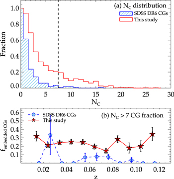
Figure 10. (a) Distribution of the number of neighboring galaxies (NC) in a comoving cylindrical volume with  and
and  for the MLCG systems (open histogram) and for the SDSS DR6 compact groups (hatched histogram). (b) The fraction of compact groups in dense environments (NC > 7) as a function of redshift: stars indicate MLCG systems and pentagons indicate SDSS DR6 compact groups.
Download figure:
Standard image High-resolution imageNC has been used as an environment measure in both theoretical and observational studies of tight galaxy pairs. For example, in a theoretical investigation, Barton et al. (2007) segregated local environments of galaxy pairs at NC = 8 and Woods et al. (2010) followed the procedure in the interpretation of observations. Woods et al. (2010) estimated that 32% of galaxy pairs are located in dense environments with NC > 8. When they computed NC, they included a pair member galaxy for counting NC; in contrast we exclude the compact group member galaxies. Thus, NC = 8 in their studies corresponds to NC = 7. Among MLCG systems, 23% are in denser regions (NC > 7), apparently somewhat lower than the fraction for galaxy pairs. However, our lower number may result from the SDSS undersampling of dense regions; this issue is much less important for pair samples from Woods et al. (2010). Woods et al. (2010) constructed pair catalogs based on the SHELS survey (Geller et al. 2005, 2014). The catalog for this survey is 97% complete to the survey limit and thus the biases are negligible.
The bottom panel of Figure 10 shows the fraction of compact groups in the denser environments as a function of redshift. The fraction changes little in the redshift range  . The fraction of MLCG systems in denser environments always exceeds that for the SDSS DR6 groups as a result of the differences in the group identification algorithm.
5. SELECTION ISSUES
5.1. Isolation Criterion
In his identification of compact groups, Hickson applied an isolation criterion to compensate for observational limitations and to avoid systems embedded in massive clusters (Hickson 1982). Barton et al. (1996) pointed out that the availability of large complete redshifts surveys obviates the need for applying an isolation criterion in the initial selection of compact group candidates. They emphasize that the large angular size of the isolation region for low-redshift systems artificially removes them from a catalog. Figure 8 of Barton et al. (1996) shows that groups with larger isolation regions have smaller sizes for groups selected from the CfA redshift survey. Here, again the limiting apparent magnitude for the definition of the isolation radius is the limiting apparent magnitude of the catalog rather than a limit three magnitudes fainter than the brightest group member. Eliminating the isolation criterion includes these nearby groups at the expense of including compact group candidates that are substructures in massive systems. However, the compact group candidates within massive systems or in dense regions can be removed after the initial selection. In contrast, the low-redshift systems cannot be recovered.
The probability of rejection as a result of the isolation criterion can increase with decreasing redshift depending on the details of the application. The lowest redshift compact group candidates have larger angular size and a correspondingly more extensive isolation region than more distant compact group candidates. Figure 7(a) shows the difference between the redshift distribution of the MLCG systems and the SDSS DR6 compact groups. Because McConnachie et al. (2009) remove r < 14.5 galaxies, they might miss some nearby groups, thus accounting for the difference. To test this conjecture, Figure 11 plots the redshift distribution of the MLCG systems containing only  galaxies in analogy with the SDSS DR6 sample. Although we remove 407 MLCG systems containing bright members, we still identify plenty of compact groups in the local universe (z < 0.05) where SDSS DR6 compact systems are absent or rare.
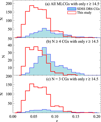
Figure 11. Redshift distribution of the MLCG systems containing only galaxies with  (open histograms) compared with the SDSS DR6 compact groups (filled histograms, Sohn et al. 2015).
Download figure:
Standard image High-resolution imageBecause we do not apply an isolation criterion in the selection algorithm, we also include compact group candidates in dense surroundings (see Figure 10). Indeed, the fraction of the MLCG systems in dense environments (NC > 7) is larger than for the SDSS DR6 compact groups at all redshifts. Interlopers may occur more often in high-density regions, thus producing some of the MLCG systems with inflated line-of-sight velocity dispersions. Barton et al. (2007) emphasize that a study of some aspects of galaxy evolution in tight pairs and compact groups requires specialization to relatively low-density environments. As in pair studies, candidate systems in dense surroundings can be removed after the general group selection.
5.2. Environmental Effects
The diverse local environments of compact groups have been discussed previously (e.g., Ramella et al. 1994; Ribeiro et al. 1998; Andernach & Coziol 2005; Mendel et al. 2011; Díaz-Giménez et al. 2012; Pompei & Iovino 2012; Díaz-Giménez & Zandivarez 2015). The fraction of embedded compact groups changes significantly depending on the group identification method and on the definition of the local environment. For example, Ramella et al. (1994) suggested that 76% of 29 Hickson compact groups are embedded, and Mendel et al. (2011) showed that 50% of the SDSS DR6 compact groups are within  Mpc of rich groups. In contrast, Pompei & Iovino (2012) found that 33% of the compact groups in the second Digitized Palomar Observatory Sky Survey (DPOSS II) are embedded in rich groups. Díaz-Giménez & Zandivarez (2015) also found that only 27% of compact groups reside in loose groups in the 2MASS compact group catalog. A direct comparison with the MLCG systems is difficult because we use a different environment measure.
Compact group properties may depend on the local environments. We compare the physical properties of groups segregated by NC in Figure 12. Panels (a)–(f) show redshift, r-band surface brightness, size, galaxy number density, velocity dispersion, and stellar mass of the MLCG systems. The plots show that properties related to the group identification, including redshift, surface brightness, size, and number density, are consistent irrespective of the local environment. In contrast with the 2MASS compact group sample (Díaz-Giménez & Zandivarez 2015), we find no dependence of the MLCG projected size on environment. The dependence found by Díaz-Giménez & Zandivarez (2015) may result from the group identification algorithm (see Section 5.1). On the other hand, the velocity dispersion and stellar mass of NC > 7 MLCG systems tend to be larger than for  groups. This result is consistent with the comparison between "isolated" and "embedded" compact groups in the DPOSS II (Pompei & Iovino 2012) and the SDSS DR6 samples (Sohn et al. 2015). These results are understandable because the interloper fraction may be enhanced in dense environments and because galaxies with greater stellar mass tend to inhabit denser regions (e.g., Bolzonella et al. 2010; Damjanov et al. 2015). Table 7 lists the range and the median of the properties of the MLCG systems in different environments.

Figure 12. Properties of compact groups as a function of environment (NC): (a) redshift, (b) surface brightness, (c) size, (d) galaxy number density, (e) velocity dispersion, and (f) stellar mass for  (open histogram) and NC > 7 (hatched histogram). The lower two panels show (g) the fraction of early- and late-type galaxies and (h) the u − r color distribution for
  and NC > 7 compact groups.
Download figure:
Standard image High-resolution imageTable 7. Comparison between Compact Groups in Different Environments
| Properties | All CGs |
 CGs CGs |
 CGs CGs |
|
|---|---|---|---|---|
| z | Range | [0.011, 0.188] | [0.014, 0.112] | [0.019, 0.112] |
| median | 0.050 ± 0.001 | 0.049 ± 0.001 | 0.053 ± 0.003 | |
| Rgr | Range | [4.9, 94.1] | [4.9, 83.7] | [8.9, 94.1] |
( kpc) kpc) |
median | 32.0 ± 0.3 | 31.8 ± 0.3 | 33.6 ± 0.8 |

|
Range | [3.29, 6.77] | [3.39, 6.77] | [3.29, 6.00] |
( ) ) |
median | 4.36 ± 0.01 | 4.37 ± 0.01 | 4.31 ± 0.03 |
| σ | Range | [1, 879] | [1, 866] | [1, 879] |
| (km s−1) | median | 194 ± 4 | 171 ± 4 | 353 ± 14 |
| fETG | 64.0 ± 0.7 | 60.4 ± 0.8 | 78.6 ± 1.3 | |
Download table as: ASCIITypeset image
We also compare the properties of member galaxies in the  and NC > 7 MLCG systems in Figures 12(g) and (h). The properties of member galaxies including the fraction of early-type galaxies and the u−r color distribution differ. The fraction of early-type galaxies is higher in NC > 7 compact groups (78.5 ± 1.3%) than in
  compact groups (60.2 ± 0.8%). The member galaxies in NC > 7 compact groups are, on average, redder than those in
  compact groups as one might expect based on the known relations between galaxy properties and local density (e.g., Park et al. 2007; Blanton & Moustakas 2009).
The differences in physical properties are qualitatively insensitive to the definition of "dense" environments for NC = 3, 5, 7, 10, 15, and 20. The MLCG systems in denser environments show larger velocity dispersion, larger stellar mass, and higher early-type fraction; other properties are essentially environment independent.
6. VOLUME-LIMITED SAMPLES
Selection of compact group candidates from a complete redshift survey offers a unique opportunity for the construction of volume-limited subcatalogs. If the underlying galaxy catalog were complete, the number density of compact groups would be a robust estimate of their true physical space density. Compact group candidates in the volume-limited catalogs V1CG and V2CG (See Section 3.2.2) should have properties that are essentially redshift independent. In contrast with the MLCG systems, comparison of the total stellar masses for the V1CG and V2CG catalogs require negligible relative correction for the unobserved portion of the mass function.
The observed number density of galaxies in the underlying volume-limited catalogs is roughly constant (Figure 13). However, the number density for both V1CG and V2CG systems declines with redshift. This decline cannot be a result of evolution; unless compact groups are replenished, their number density must decline with cosmic time (Diaferio et al. 1994). For the V1CG systems the decline in Figure 13 begins at  for the V2CG systems it begins at z ∼ 0.07. This behavior reflects the impact of the SDSS fiber-positioning constraints. Shen et al. (2016) showed that the fraction of missing close pairs is a function of both redshift and apparent magnitude. The number density of the V2CG systems declines significantly at a redshift where the fiber exclusion radius of 55ʺ becomes comparable with the projected linking length of
  we apply. This behavior is similar to the behavior in Figure 2 of Shen et al. (2016). The steeper decline for the V1CG systems probably reflects the selection against the lower luminosity objects in these groups.

Figure 13. Abundance of the MLCG systems (filled circles), V1CG systems (filled triangles), and V2CG systems (filled stars) as a function of redshift. We also plot the abundance of V1 galaxies (open triangles) and V2 galaxies (open stars); these number densities are nearly constant as expected. The number densities of the compact group samples decline artificially with redshift because of SDSS fiber-positioning constraints.
Download figure:
Standard image High-resolution imageAs a result of the fiber-positioning constraints, we cannot be confident that the compact group catalog is complete at any redshift. However, it is interesting to note that the number density at the lowest redshifts is consistent with previous determinations (Mendes de Oliveira & Hickson 1991; Barton et al. 1996; Sohn et al. 2015). Figure 13 also shows number density estimates for Mendel et al. (2011) and Pompei & Iovino (2012) catalogs. These abundances appear to track the artificially declining abundance of the MLCG. This consistency suggests that the previous catalogs may also be incomplete.
Although the volume-limited samples are not complete, they still provide a set of systems with a similar range of physical properties throughout the sample redshift range. Figure 14 shows normalized histograms of the distributions of properties for the MLCG, V1CG, and V2CG catalogs. The difference in redshift distribution simply reflects the selection. The distribution of velocity dispersions for the V2CGs appears double peaked. The groups in the higher velocity dispersion peak are typically in denser regions with NC ∼ 5. As expected based on the selection, the V2CG systems have larger total stellar masses than the V1CG systems. The low stellar mass tail present among the MLCG systems is absent from the volume-limited samples.

Figure 14. Comparison of physical properties of the MLCG systems (open histograms), V1CGs (hatched histograms), and V2CGs (filled histograms) including (a) mean redshift, (b) line-of-sight velocity dispersion (σCG), (c) physical radius, (d) galaxy number density, (e) total stellar mass, and (g) fraction of early-type galaxies.
Download figure:
Standard image High-resolution imageFigure 15 provides a qualitative guide to some of the interesting properties of the candidate systems in the catalog. Systems with low line-of-sight velocity dispersion ( ) are a prior likely to be bound. Remarkably, the montage in Figure 15 shows that nearly all of these systems, even with the shallow SDSS photometry, show signs of dynamical interaction. Late-type galaxies often have tidal tails (e.g., panel 11, 14, 15, and 19); early-type galaxies are often apparently embedded in a common halo (e.g., panel 12, 13, 16, 18, and 20). Each panel of the montage lists NC. Most of these objects have low NC, suggesting that they are excellent candidates for the study of relatively isolated, probably interacting/merging systems. V1CG189 is the main exception with an NC = 7; it is probably a substructure in a richer system.
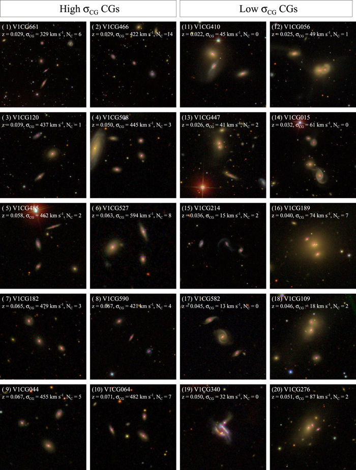
Figure 15. Sample images of V1CGs. The left two columns show examples with  . The right two columns show images of groups with
  .
.
Download figure:
Standard image High-resolution imageIn contrast, systems with high velocity dispersion ( ) show little or no evidence of obvious dynamical interaction. It is interesting to note that the range of NC for these systems is larger than for the massive systems; three of these example systems have
  . In these cases, the velocity dispersion may well be inflated by one or more interlopers from the cluster. It is also possible that galaxies in the high velocity dispersion systems interact with each other at high relative velocities. Fast encounters tend to produce less prominent interaction features than the slower encounters in the lower velocity dispersion groups. Deeper observations might reveal more subtle features of interactions, but with the current data there is no way of judging whether the system is a true bound system. For velocity dispersions
  , the candidate systems show a mix of qualitative visual properties along with a mix of environments.
The volume-limited samples provide a platform for more detailed studies of the physical properties of a homogeneous sample of compact group candidates including spectroscopic properties, dynamical studies (e.g., Barton et al. 1996; Pompei & Iovino 2012; Sohn et al. 2015), deeper photometric observations (e.g., Brosch 2015), and observations in other wavebands from the radio to the X-ray (e.g., Desjardins et al. 2014; Walker et al. 2016). Many of these groups have an angular size comparable to the MANGA field of view (∼32'', Bundy et al. 2015). Thus, detailed spatially resolved spectroscopy of these systems could provide fresh insight into the apparent dynamical interactions among the members.
7. CONCLUSION
We apply an FoF method to an enhanced SDSS DR12 spectroscopic catalog to construct a catalog of 1588  compact groups containing 5178 member galaxies and covering the redshift range 0.01 < z < 0.19. The approach to the construction of this catalog is similar to Barton et al. (1996). However, the new catalog contains 18 times as many systems and reached to three times the depth. These two catalogs are unique in their derivation from dense and nearly complete redshift surveys. The general properties of these spectroscopic compact groups including their velocity dispersions, sizes, densities, and galaxy population are similar to those previously selected from photometric data sets.
We use a fixed projected physical spatial and rest-frame line-of-sight velocity linking lengths to generate a catalog where group projected size and density are redshift independent. Even with fixed selection parameters, a frequently applied isolation criterion produces an artificial increase in compact group size with redshift in some other previous catalogs.
Application of an isolation criterion can also mitigate against the inclusion of nearby groups in a catalog, depending on the details of the application. The catalogs we construct contain many more compact group candidates at z ≲ 0.05 than previous catalogs. Many of these systems show obvious evidence for current tidal interactions among the member galaxies.
When we explore the catalog as a whole, the fraction of obviously interacting systems is striking for groups with velocity dispersions ≲100  . For group candidates with the largest dispersions (
 ), there is little evidence for these interactions, perhaps suggesting some interloper contamination. Deeper photometric observations are necessary to explore this issue further.
The catalog includes systems in a range of environments. Group properties depend somewhat on the environment in the sense that groups in dense environments contain a larger fraction of early-type galaxies as expected.
In contrast, with earlier investigations, we construct volume-limited catalogs in addition to the primary magnitude-limited sample. The volume-limited catalogs have several important advantages. The systems should have similar physical properties throughout the redshift range. Unlike the systems in the magnitude-limited catalog, the volume-limited systems have total stellar masses nearly independent of redshift. It is important here that there is little correction for the missing end of the mass function because the samples are volume-limited.
The volume-limited samples are potentially powerful probes of the number density of compact groups. At low redshift our number density  agrees with Mendes de Oliveira & Hickson (1991) and Barton et al. (1996). The volume-limited sample number density as a function of redshift provides an important probe of the impact of the SDSS fiber placement constraint; a decline in the number density is apparent at redshifts corresponding to the constraint. This fiber placement constraint is currently a fundamental limitation on the interpretation of the number density as a function of redshift. Eliminating this issue (see Shen et al. 2016) could enable insights into the number density evolution of compact groups based on volume-limited samples.
The abundant systems in the volume-limited compact group catalogs at  offer a rich foundation for detailed investigations of spatially resolved spectroscopic measures of star formation histories and stellar population ages. At these redshifts the surface brightness of tidal features is high enough to support extensive exploration of the internal galaxy kinematics. Taken together, dynamical studies coupled with other age indications may provide a route to solving the mystery of the existence of compact groups.
This work was supported by the National Research Foundation of Korea (NRF) grant funded by the Korea Government (MSIP) (No.2013R1A2A2A05005120). J.S. was supported by the Global Ph.D. Fellowship Program through an NRF funded by the MEST (No. 2011-0007215). The research of J.S., M.J.G., and H.J.Z. is supported by the Smithsonian Institution. H.J.Z. gratefully acknowledges the support of the Clay Fellowship.
Funding for SDSS-III has been provided by the Alfred P. Sloan Foundation, the Participating Institutions, the National Science Foundation, and the U.S. Department of Energy Office of Science. The SDSS-III website is www.sdss3.org/. SDSS-III is managed by the Astrophysical Research Consortium for the Participating Institutions of the SDSS-III Collaboration including the University of Arizona, the Brazilian Participation Group, Brookhaven National Laboratory, Carnegie Mellon University, University of Florida, the French Participation Group, the German Participation Group, Harvard University, the Instituto de Astrofisica de Canarias, the Michigan State/Notre Dame/JINA Participation Group, Johns Hopkins University, Lawrence Berkeley National Laboratory, Max Planck Institute for Astrophysics, Max Planck Institute for Extraterrestrial Physics, New Mexico State University, New York University, Ohio State University, Pennsylvania State University, University of Portsmouth, Princeton University, the Spanish Participation Group, University of Tokyo, University of Utah, Vanderbilt University, University of Virginia, University of Washington, and Yale University.
APPENDIX: COMPACT GROUP CANDIDATES ELIMINATED BY POPULATION AND SURFACE BRIGHTNESS SELECTION
In the construction of the MLCG catalog we do not apply Hickson's original isolation criterion (See Section 3.1). We do, however, apply the "population" criterion ( ). This criterion removes 294 systems that include a bright galaxy surrounded by much fainter apparent satellite galaxies at very similar redshift. We also apply Hickson's "compactness" criterion (
 , which excludes a further 109 groups. This criterion excludes systems containing galaxies of much lower surface brightness than the typical systems over the redshift range covered by the MLCG. Here we briefly examine subsets of the systems removed by these two criteria. These systems may be useful for applications other than the study of traditional compact group candidates.
Figure 16 shows example images of some the systems that violate the "population" criterion. As these images show, these objects have one dominant bright galaxy surrounded by much fainter satellites. Unlike the more standard compact group candidates we discuss in the body of this paper, these group candidates are not comprised of galaxies with comparable stellar masses.
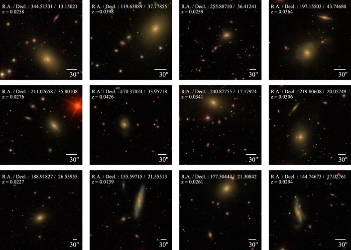
Figure 16. Sample images of compact group candidates rejected by the population criterion. They contain member galaxies differing from the brightest member by  . Magenta symbols mark the member galaxies. The white bar shows a 30ʺ scale at the mean group redshift.
Download figure:
Standard image High-resolution imageSystems like those in Figure 16 have been the basis for investigating the dark matter halo of the dominant galaxy (Zaritsky et al. 1993; Norberg et al. 2008; Wojtak & Mamon 2013). To measure the distribution of dark matter in the dominant galaxy halo, Zaritsky et al. (1993) compiled the redshifts for the satellites of 45 apparently isolated spiral galaxies; the typical systems they investigated have one to four satellites. Other investigators have since used larger samples satellites to revisit the constraints on the mass distribution in galaxy dark matter halos (Holmberg 1969; Sales & Lambas 2005; Prescott et al. 2011; Wang et al. 2014). The FoF we apply to the SDSS DR12 yields 294 similar systems that could be used for further investigation of these issues. We include the catalog in Tables 8 and 9.
Table 8. Catalog of System Containing a Dominant Galaxy Surrounded by Satellites
| R.A. | Decl. |

|
Redshift |
|---|---|---|---|
| 198.227158 | 1.012775 | 3 | 0.0723 |
| 141.442184 | 11.437011 | 3 | 0.0113 |
| 127.134727 | 30.435843 | 4 | 0.0506 |
| 188.723557 | 47.756451 | 3 | 0.0306 |
| 187.538025 | 47.021252 | 3 | 0.0394 |
Only a portion of this table is shown here to demonstrate its form and content. A machine-readable version of the full table is available.
Download table as: DataTypeset image
Table 9. Catalog of Galaxies in the System Containing a Dominant Galaxy Surrounded by Satellites
| Object ID | R.A. | Decl. | r | Redshift |
|---|---|---|---|---|
| 1237648705657307347 | 198.229294 | 1.010990 | 17.42 | 0.0727 ± 0.00002 |
| 1237648705657307315 | 198.218872 | 1.019821 | 16.48 | 0.0704 ± 0.00002 |
| 1237661070318370904 | 141.447220 | 11.424596 | 12.45 | 0.0125 ± 0.00001 |
| 1237661070318370911 | 141.452072 | 11.454233 | 15.11 | 0.0108 ± 0.00001 |
| 1237661070318370902 | 141.427277 | 11.432204 | 11.76 | 0.0107 ± 0.00004 |
Only a portion of this table is shown here to demonstrate its form and content. A machine-readable version of the full table is available.
Download table as: DataTypeset image
Figure 17 displays examples of the 109 systems eliminated from compact group catalog because of their low surface brightness. These systems are comprised of small, low-luminosity galaxies. These candidate systems show no obvious sign of recent interaction/merger in the SDSS images. The search radius we use is essentially tuned to find dense systems of galaxies with stellar masses  . Finding candidate interacting systems of low-luminosity objects probably requires tighter selection criteria. These systems are rare in our catalog because they are only visible in the lowest redshift portion of the catalog; their maximum redshift is z = 0.05 and most of them have redshifts around z ∼ 0.03. For completeness we include these objects in Tables 10 and 11.
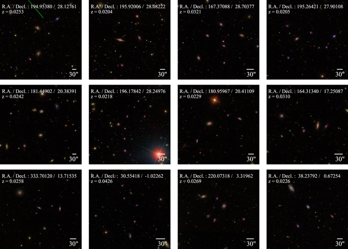
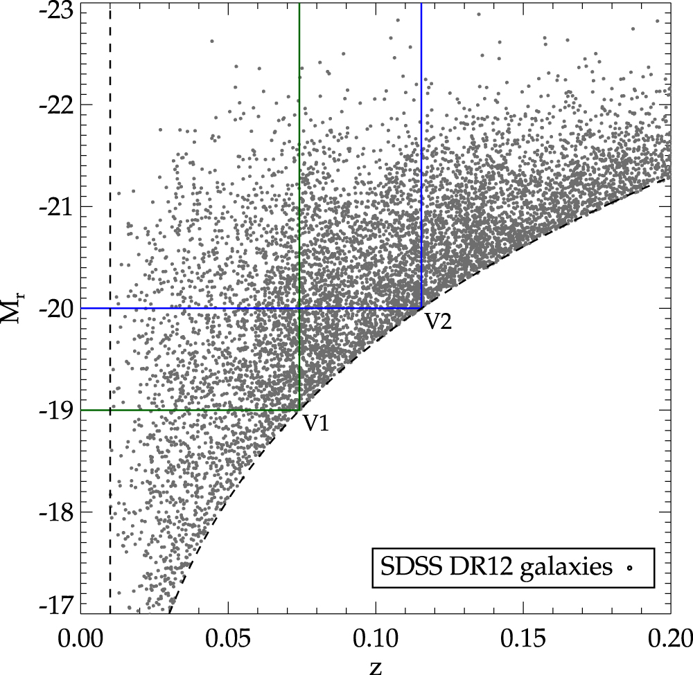
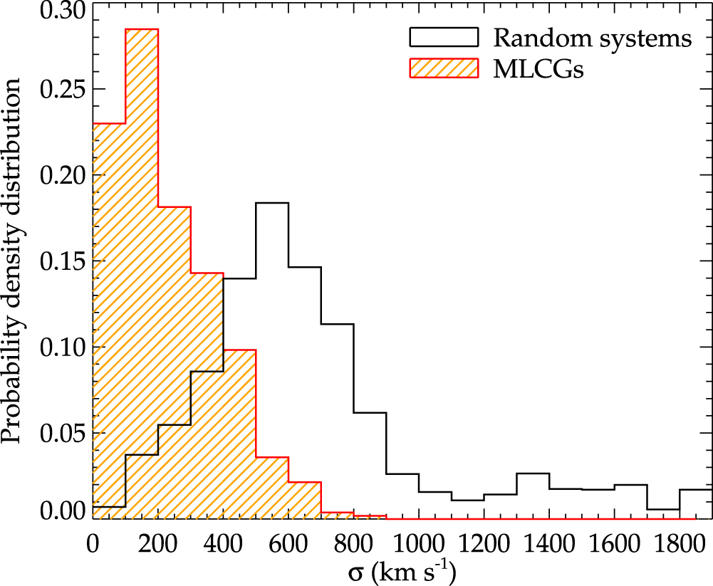
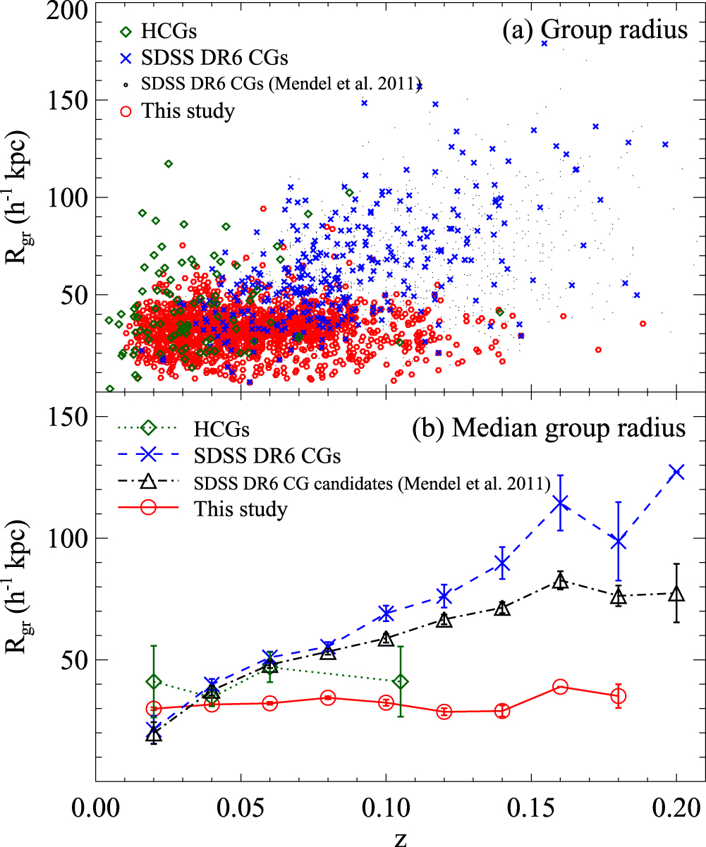
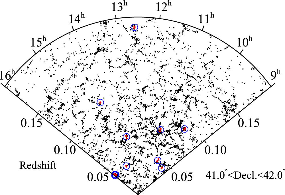
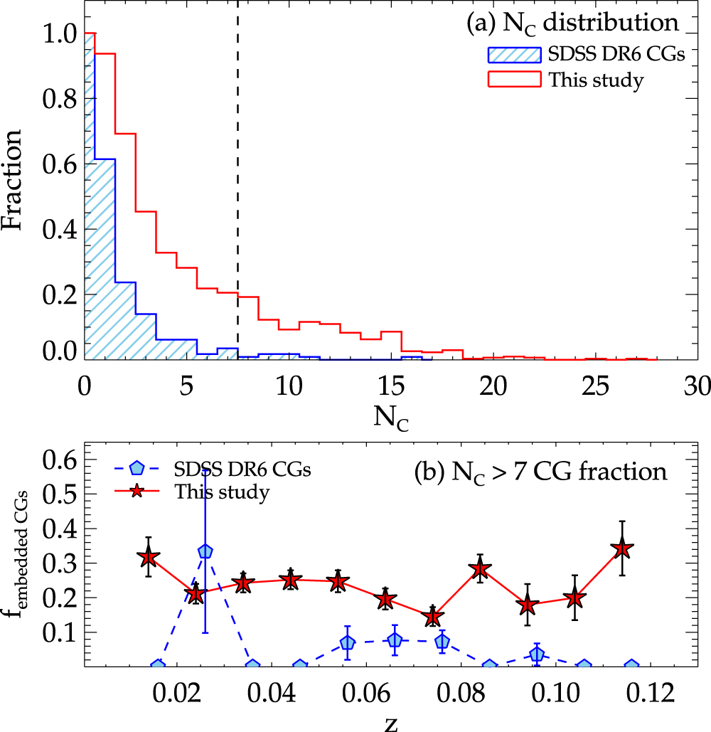
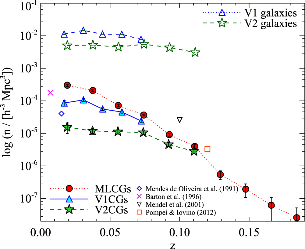
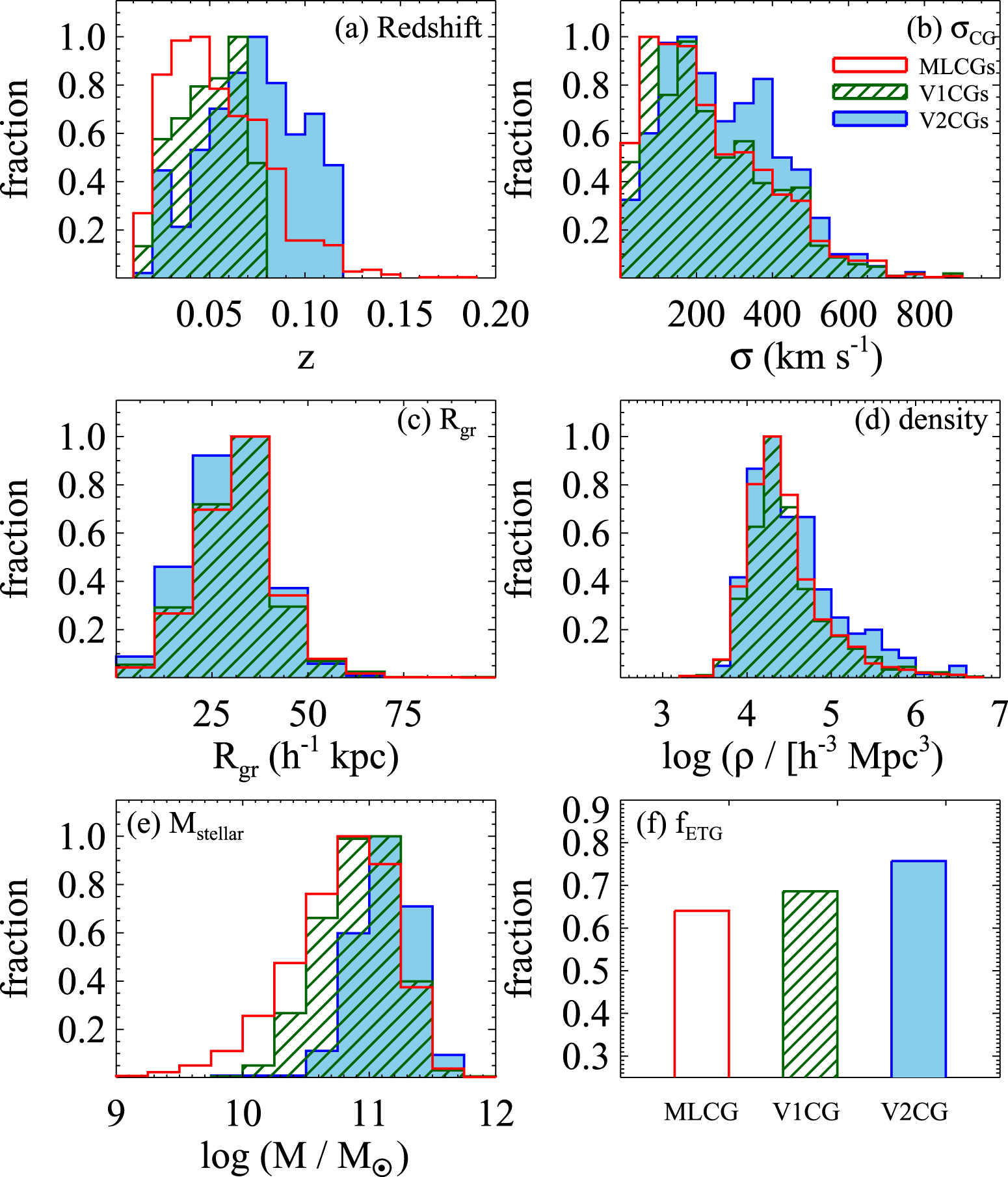
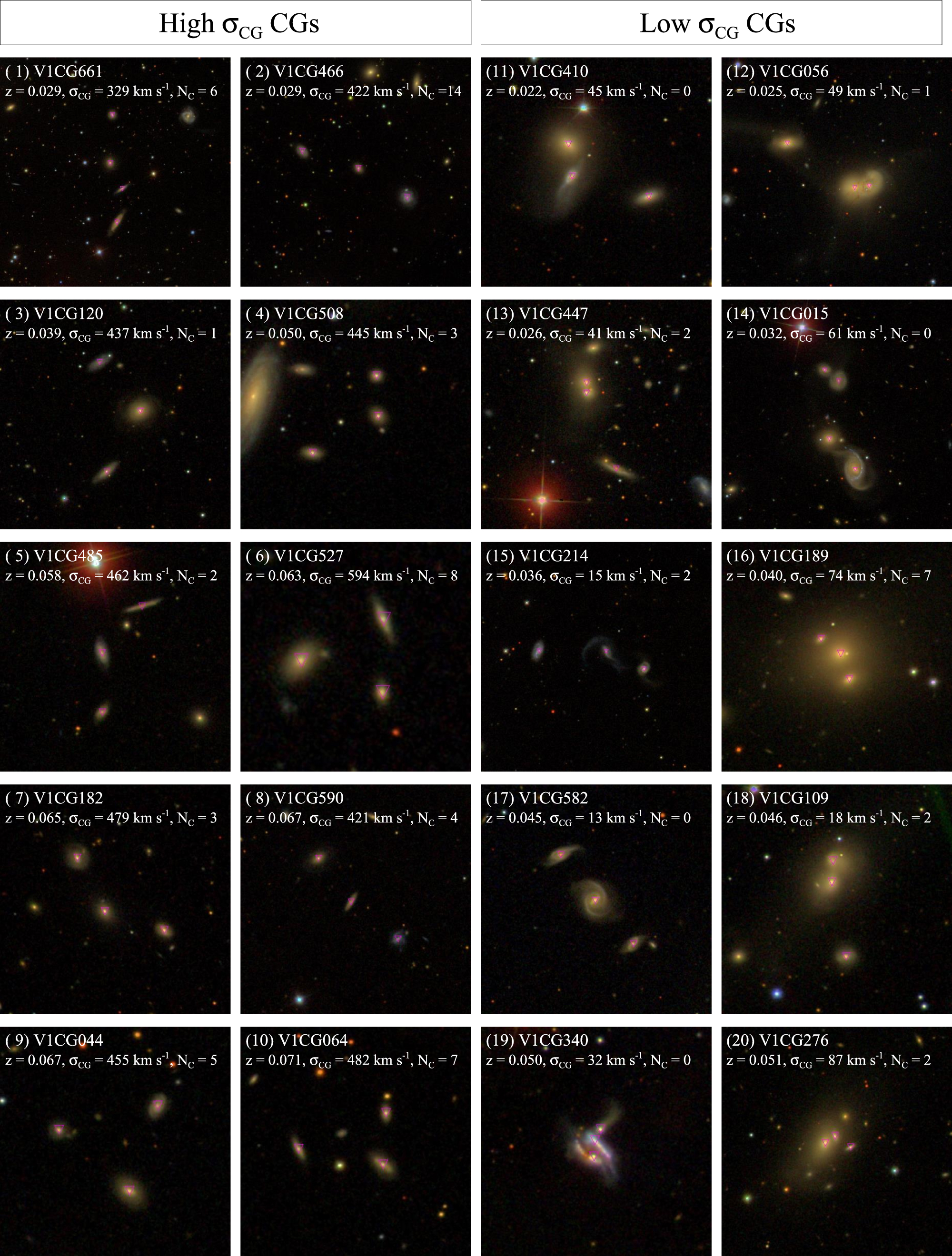
Figure 17. Sample images of compact group candidates rejected by the surface brightness criterion:  . The magenta symbol and the white bar have the same meaning as in as Figure 16.
Download figure:
Standard image High-resolution image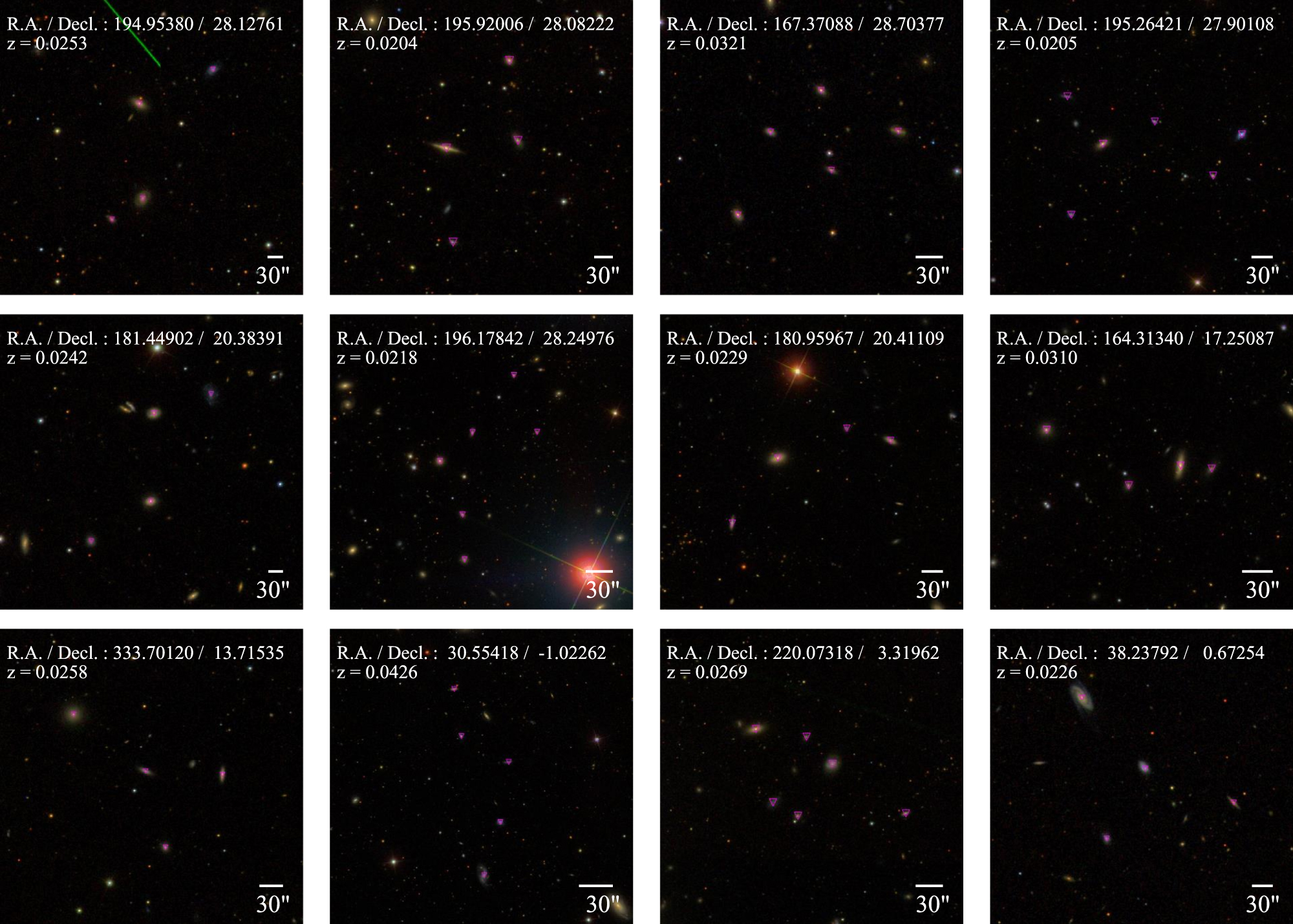
Table 10.
Catalog of System with Low Surface Brightness ( )
)
| R.A. | Decl. |

|
Redshift |
|---|---|---|---|
| 140.011292 | 33.666660 | 5 | 0.0222 |
| 141.283279 | 11.557135 | 3 | 0.0121 |
| 247.183990 | 39.646721 | 7 | 0.0292 |
| 149.441193 | 36.060726 | 3 | 0.0267 |
| 247.305191 | 39.599922 | 4 | 0.0327 |
Only a portion of this table is shown here to demonstrate its form and content. A machine-readable version of the full table is available.
Download table as: DataTypeset image
Table 11.
Catalog of Galaxies in Systems with Low Surface Brightness ( )
)
| Object ID | R.A. | Decl. | r | Redshift |
|---|---|---|---|---|
| 1237661383844036884 | 140.035767 | 33.661671 | 15.27 | 0.0207 ± 0.00001 |
| 1237661383844036895 | 140.053909 | 33.631790 | 16.84 | 0.0221 ± 0.00001 |
| 1237661126155436283 | 139.988480 | 33.679878 | 17.70 | 0.0226 ± 0.00002 |
| 1237661126155501585 | 140.010468 | 33.710468 | 14.28 | 0.0233 ± 0.00001 |
| 1237664870286098561 | 139.967880 | 33.649494 | 15.13 | 0.0222 ± 0.00001 |
Only a portion of this table is shown here to demonstrate its form and content. A machine-readable version of the full table is available.
Download table as: DataTypeset image