


ABSTRACT
We have obtained a deep X-ray image of the nearby galaxy M51 using Chandra. Here we present the catalog of X-ray sources detected in these observations and provide an overview of the properties of the point-source population. We find 298 sources within the D25 radii of NGC 5194/5, of which 20% are variable, a dozen are classical transients, and another half dozen are transient-like sources. The typical number of active ultraluminous X-ray sources in any given observation is ∼5, and only two of those sources persist in an ultraluminous state over the 12 yr of observations. Given reasonable assumptions about the supernova remnant population, the luminosity function is well described by a power law with an index between 1.55 and 1.7, only slightly shallower than that found for populations dominated by high-mass X-ray binaries (HMXBs), which suggests that the binary population in NGC 5194 is also dominated by HMXBs. The luminosity function of NGC 5195 is more consistent with a low-mass X-ray binary dominated population.
Export citation and abstract BibTeX RIS
1. INTRODUCTION
M51 (NGC 5194/5)5 is a nearly face-on grand-design spiral at a distance of approximately 7.6 Mpc (Ciardullo et al. 2002). The strongly defined spiral arms have made M51 the textbook exemplar for the properties of spiral galaxies (Toomre 1981), from the correlation of atomic and molecular gas (e.g., Louie et al. 2013) to the direction of magnetic fields (Neininger & Horellou 1996). NGC 5194's interaction with the nearby NGC 5195 makes M51 one of the closer examples of galaxy–galaxy interaction and the test case, if not inspiration, for models of spiral structure. Its low-luminosity Seyfert 2 nucleus (Rose & Searle 1982) may be the closest of its type. Yet despite its iconic nature, M51 is still poorly understood, lacking even a Cepheid determined distance. M51 is considered a "quiescently" star-forming system (Calzetti et al. 2004) but, despite its star formation rate, has had at least four supernovae since 1941. Thus, one would expect M51 to be an important observational laboratory for supernovae and supernova remnants (SNRs), yet there has been no catalog of remnants in this galaxy. Similarly, despite extensive studies of the cold interstellar medium (ISM), particularly with respect to star formation (e.g., Leroy et al. 2008; Meidt et al. 2013; Colombo et al. 2014, among many others), there has been little study of the hot ISM produced as a result of that star formation.
To fill in the crucial high-energy gap in the coverage of M51, and to address a variety of science questions, we obtained 745 ks of new Chandra observations, which, when combined with the 107 ks of Chandra archival observations, provide a data set comparable to those of other nearby galaxies (Kuntz & Snowden 2010; Tüllmann et al. 2011; Long et al. 2014). M51 is particularly well suited for Chandra observations: the foreground absorption due to gas within the Milky Way is low, with NH of ∼1.9 × 1020 cm−2 (Kalberla et al. 2005). Its size, 11 2 × 69 (de Vaucouleurs et al. 1991), is only slightly larger than the soft X-ray sensitive ACIS S3 field of view (FOV). The galaxy is roughly face-on, so the relation of the sources to the underlying galactic structure is unambiguous. The relevant properties of NGC 5194, and NGC 5195 are listed in Table 1. As a foundation for a series of deeper studies of the point-source populations, the SNR population, and the diffuse emission, this work presents the catalog of point and point-like sources.
Table 1. Properties of NGC 5194/5195
| Property | Value | Reference | |
|---|---|---|---|
| NGC 5194 | NGC 5195 | ||
| Type | SA(s)bc/Sy 2 | I0 | de Vaucouleurs et al. (1991) |
| Distance | 7.6 Mpc | 7.6 Mpc | Ciardullo et al. (2002) |
| Foreground NH | 2 × 1020 cm−2 | 2 × 1020 cm−2 | Kalberla et al. (2005) |
| D25 | 112 × 69 |
58 × 46 |
de Vaucouleurs et al. (1991) |
| Position Angle | 163° | 79° | de Vaucouleurs et al. (1991) |
| Inclinationa | 22 ± 5 | ... | Colombo et al. (2014) |
| Position Anglea | 173 ± 3 | ... | Colombo et al. (2014) |
| Scale Lengthb | 108 1 ± 149 1 ± 149 |
... | Beckman et al. (1996) |
| SF Rate | 2.7 M☉ yr−1 | ... | Jarrett et al. (2013)c |
| log(M*) | 10.6 | ... | Leroy et al. (2008) |
| log(MH i) | 9.5 | ... | Leroy et al. (2008) |
log(M ) ) |
9.4 | ... | Leroy et al. (2008) |
Notes.
aDerived from dynamical data. bB band. cCorrected from their adopted distance to 7.6 Mpc. We note that there is a large spread of values in the current literature; we have chosen the value from Jarrett et al. (2013) so that there can be a consistent comparison among galaxies that have very deep Chandra data (M51, M83, and M101). The Jarrett et al. (2013) measure of the star formation used WISE and GALEX data. We note that this value of the star formation rate is comparable to those found by the same authors for M83 (3.06 M☉ yr−1 at 4.6 Mpc) and M101 (2.94 M☉ yr−1 at 6.8 Mpc) when corrected to the current understanding of the distances to these galaxies.Download table as: ASCIITypeset image
Previous observations: Early observations of M51 with Einstein and ROSAT revealed the existence of a small number of very luminous sources (brighter than the Eddington limit for 1 M☉), as well as extended emission from the nucleus. Intercomparison of ROSAT observations suggested little variability, while comparison of ROSAT with Einstein was equivocal (Ehle et al. 1995; Marston et al. 1995). Given the comparatively poor angular resolution of ROSAT, there was concern that the bright sources might be either extended emission or aggregates of point sources. Terashima & Wilson (2004) confirmed that M51 has a much larger population of ultraluminous X-ray sources (ULX) than did the typical spiral galaxy, even though some of the previously cataloged sources were aggregates. Terashima & Wilson (2004) also cataloged 96 sources projected onto M51, while Terashima & Wilson (2001) studied only the bright nucleus and extended nuclear emission. Kilgard et al. (2005) reanalyzed the first two Chandra observations and demonstrated that the luminosity function has a slope of ∼1.7, comparable to other strongly star-forming galaxies.
Here we provide an overview of a very deep set of Chandra observations of M51 and the construction of a catalog of its X-ray point sources. The remainder of the paper is organized as follows: Section 2 describes the data, Section 3 describes the catalog construction, Section 4 describes the cross-correlation with multiwavelength catalogs and other sources of source identification, Section 5 describes the gross properties of the source population, including the luminosity functions, and Section 6 describes the nuclear region.
2. OBSERVATIONS AND REDUCTION
2.1. Chandra
This deep study of M51 is composed of 107 ks of archival observations, to which we have added another 745 ks of observations. All of the observations were made with the ACIS-S array. The archival observations were made with a variety of pointing centers and roll angles. The new observations were made with the aim point (the location with the smallest point-spread function [PSF]) near the nucleus of the galaxy, and the roll was set to place the center of the S3 chip near the northern arm. As can be seen in Figure 1, the bulk of the D25 radius is covered by the backside-illuminated S3 chip. Both the new and archival data were reprocessed with CIAO version 4.6 and CalDB version 4.6.3. We used light curves in the 2–7 keV band to check for and remove soft proton flares. With the exception of ObsID 3932, which lost roughly 2 ks to flares, there were no other signficant losses due to flares. The new observations include the longest single exposure and, despite the continued loss of effective area due to the buildup of hydrocarbons on the entrance window, the single deepest exposures in 0.5–2.0 keV as well. A list of the observations used is given in Table 2.
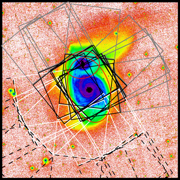
Figure 1. SDSS z-band image of M51. Overlayed are the FOV of the ACIS-S chips: S4 (gray), S3 (solid black), S2 (white), and S1 (dashed black). The red ellipses are the D25 regions for NGC 5194 and its smaller companion, NGC 5195. The image has been logarithmically stretched to accentuate the plumes to the northwest and southeast of NGC 5194.
Download figure:
Standard image High-resolution imageTable 2. Chandra Observations
| ObsID | Date | Major | Expo. | Roll | Mode |
|---|---|---|---|---|---|
| Epoch | Time | Angle | |||
| (ks) | (deg) | ||||
| 354 | 2000 Jun 20T08:03:51 | A | 14.86 | 237.76 | FAINT |
| 1622 | 2001 Jun 23T18:47:13 | B | 26.81 | 240.09 | VFAINT |
| 3932 | 2003 Aug 07T14:31:44 | C | 45.83 | 276.75 | VFAINT |
| 12562 | 2011 Jun 12T06:52:28 | D | 9.63 | 231.10 | VFAINT |
| 12668 | 2011 Jul 03T10:31:57 | D | 9.99 | 246.90 | VFAINT |
| 13812 | 2012 Sep 12T18:24:56 | E | 157.46 | 316.15 | FAINT |
| 13813 | 2012 Sep 09T17:48:37 | E | 179.20 | 316.15 | FAINT |
| 15496 | 2012 Sep 19T09:21:41 | E | 40.97 | 330.14 | FAINT |
| 13814 | 2012 Sep 20T07:22:49 | E | 189.85 | 330.14 | FAINT |
| 13815 | 2012 Sep 23T08:13:15 | E | 67.18 | 335.01 | FAINT |
| 13816 | 2012 Sep 26T05:12:47 | E | 73.10 | 335.01 | FAINT |
| 15553 | 2012 Oct 10T00:44:42 | E | 37.57 | 351.73 | FAINT |
Download table as: ASCIITypeset image
Figure 2 is a three-band color X-ray image of the central part of the Chandra FOV. As usual, the red band is the softest (S, 0.35–1.1 keV), green is the intermediate band (M, 1.1–2.6 keV), and blue is the hardest (H, 2.6–8.0 keV). The bulk of the diffuse disk emission appears only in the softest band, though diffuse emission contributes significantly to the intermediate band in the nuclear region of both galaxies. In this image, a point source having the same number of counts in each band appears white. For reference, a source with Γ = 1.9 and an absorption by 2 × 1020 cm−2 has a ratio of 203:258:89 counts s−1 in the three bands and would be yellow; harder sources are blue.
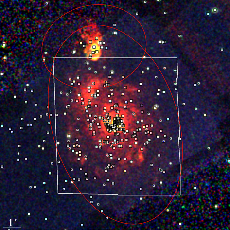
Figure 2. Three-color broadband X-ray mosaic of M51. The broad bands displayed are 0.35–1.1 keV (red), 1.1–2.6 keV (green), and 2.6–8.0 keV (blue). Also shown are the locations of the point sources, the D25 region, and the location of the HST mosaic shown in the following figure.
Download figure:
Standard image High-resolution imageIn order to align the Chandra observations with one another and reduce the effective PSF for sources in the overlap regions, we created a point-source list, covering all of the active chips, from each observation. Comparing these lists allowed us to use the sources in the region of overlap to determine the relative offsets between observations. The mean offset from the longest observations was ≲0.41 pixels (020).
We aligned our Chandra coordinates to an absolute coordinate frame in a two-step process. Since we are most interested in identifying optical counterparts to X-ray sources in the Hubble Space Telescope (HST) images, we corrected the Chandra coordinates to those of the HST images, which had in turn been corrected to the Two Micron All Sky Survey (2MASS) coordinate frame. We searched the HST F814W mosaic for close matches (<10) between X-ray sources and isolated foreground stars and compact background galaxies. We found 20 candidate matches: three foreground stars, with the remainder being background galaxies. After correcting the Chandra coordinates to match the HST coordinates, 17 of those matches had offsets of <033, while the remaining three sources were clearly outliers. The mean offset between Chandra and HST sources was 014, significantly smaller than a Chandra pixel (0492) but significantly larger than the HST pixel (00396).
2.2. HST
M51 has been observed extensively with HST. In particular, essentially all of M51 and its companion NGC 5195 was imaged with Advanced Camera for Surveys (ACS) in V, R, and I (F435W, F555W, F814W) and Hα (F658N) as a Hubble Legacy Project (Proposal ID 10452, PI: Steve Beckwith).6
For our work on M51, we have reprocessed the data obtained in the Legacy program, correcting all of the images for charge transfer inefficiency, using the software available in 2013. We then used AstroDrizzle (Version 1.1.10) to combine the images into mosaics and to place all of the various filters on a common astrometric system. The F814W images were combined first, and the absolute coordinate system was established using a combination of UCAC3 and 2MASS stars. The images from the other filters were then aligned to the F814W mosaic, so that all of the images are aligned with one another. The absolute astrometric error in the HST mosaics used here should be significantly less than 01. The HST image and the location of the X-ray point sources is shown in Figure 3.
3. THE X-RAY POINT-SOURCE CATALOG
3.1. Generation
As indicated in Section 2.1 and as can be seen in Figure 2, the X-ray emission from M51 is complex; the highest surface density of sources is often in regions with strong diffuse emission, so crowding is often exacerbated by a bright irregular background. The well-known variation of the Chandra PSF with radius, in combination with multiple observations with different pointing positions and roll angles, makes the PSF of any single source quite complex. To address these complixities here, we have made use of a combination of CIAO tools and the ACIS Extract (AE; Broos et al. 2010) software package. We used a procedure very similar to that used by Long et al. (2014) and earlier by Tüllmann et al. (2011) in their studies of M83 and M33, respectively.
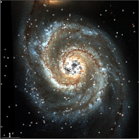
Figure 3. Three-color broadband optical mosaic of M51 showing the location of the point sources. The three HST broadband images used are F435W (blue), F555W (green), and F814W (red).
Download figure:
Standard image High-resolution imagePoint-source detection was done with the CIAO wavdetect routine for a series of overlapping bands for each chip of each individual observation. The detection bands included all those listed in Table 3, as well as the 0.45–0.70 keV and 0.70–1.0 keV bands. The point-source detection was then done for the same bands for all of the observations combined. All of these lists were then merged to produce a single source list. We also closely examined the images for any sources that might have been missed, and we added those few sources to the list. Since the sigthresh parameter for wavdetect was set to 10−6, we expect roughly one statistically spurious detection per chip, per band, per observation. This produces on the order of 250 spurious detections. Further, since the size of the PSF changes over each chip, the source detection must be sensitive to scales slightly larger than the largest PSF, which can be significantly larger than the smallest PSF. For an "empty sky" image, this is of little import, but for a galaxy with significant diffuse emission, it causes the detection of variation in the diffuse background as point sources. Thus, one expects the initial catalog to contain a large number of spurious detections, which must be removed at a later stage of catalog construction. The nuclear region is particularly problematic in this regard; the construction of the point-source catalog in this region is discussed in detail in Section 6.
Table 3. Source Statistics
| Band | Energy | Number | Long-term Variation | Medium-term Variation | |||||||||
|---|---|---|---|---|---|---|---|---|---|---|---|---|---|
| Fraction | Limiting Flux | Fraction | Limiting Flux | ||||||||||
| Variable | for Frac. Var. | Variable | for Frac. Var. | ||||||||||
| Total | <D25 | Total | <D25 | 25% | 50% | 100% | Total | <D25 | 25% | 50% | 100% | ||
| (keV) | (photon cm−2 s−1) | (photon cm−2 s−1) | |||||||||||
| S | 0.35–1.1 | 308 | 203 | 0.16 | 0.21 | 2.3 × 10⁻⁶ | 3.3 × 10⁻⁷ | 8.3 × 10⁻⁸ | 0.06 | 0.05 | 3.1 × 10⁻⁶ | 6.9 × 10⁻⁷ | 1.1 × 10⁻⁷ |
| M | 1.1–2.6 | 393 | 216 | 0.17 | 0.25 | 1.9 × 10⁻⁶ | 2.1 × 10⁻⁷ | 5.8 × 10⁻⁸ | 0.12 | 0.12 | 1.4 × 10⁻⁶ | 3.1 × 10⁻⁷ | 0.58 × 10⁻⁷ |
| H | 2.6–8.0 | 229 | 118 | 0.12 | 0.23 | 4.1 × 10⁻⁶ | 3.8 × 10⁻⁷ | 1.2 × 10⁻⁷ | 0.14 | 0.17 | 6.7 × 10⁻⁶ | 6.4 × 10⁻⁷ | 1.3 × 10⁻⁷ |
| T | 0.35–8.0 | 488 | 280 | 0.17 | 0.23 | 2.5 × 10⁻⁶ | 5.1 × 10⁻⁷ | 1.0 × 10⁻⁷ | 0.13 | 0.13 | 2.6 × 10⁻⁶ | 4.9 × 10⁻⁷ | 1.1 × 10⁻⁷ |

|
0.5–2.0 | 430 | 257 | 0.17 | 0.24 | 2.2 × 10⁻⁶ | 2.3 × 10⁻⁷ | 6.0 × 10⁻⁸ | 0.11 | 0.10 | 1.9 × 10⁻⁶ | 4.0 × 10⁻⁷ | 0.68 × 10⁻⁷ |

|
2.0–8.0 | 263 | 135 | 0.14 | 0.24 | 3.8 × 10⁻⁶ | 3.8 × 10⁻⁷ | 1.1 × 10⁻⁷ | 0.17 | 0.20 | 2.4 × 10⁻⁶ | 7.8 × 10⁻⁷ | 1.3 × 10⁻⁷ |
| Any | ⋯ | 503 | 298 | 0.20 | 0.24 | ⋯ | ⋯ | ⋯ | 0.13 | 0.08 | ⋯ | ⋯ | ⋯ |
Download table as: ASCIITypeset image
We used AE to perform the photometry. For each source, AE extracted a source region whose size and shape were based on the local PSF, and a background region whose size and shape were based on the size of the local PSF and the location of nearby sources. Source properties were then calculated in a standard manner.7 Of particular importance in this analysis is the prob_no_source parameter, which is the probability that one could measure the observed count rate in the absence of a source. We have taken a source to be significant only if this parameter is <5 × 10⁻⁶. At this probability threshold one would expect a single spurious source per field, or roughly 1.5 sources within the D25. As we used the same value in our analysis of M83, the two catalogs are directly comparable.
In the presence of a significant number of spurious sources, the area of the background regions will be significantly reduced by AE, and the statistics in the measure of the background will be poorer. Thus, to improve the background statistics, once we removed spurious sources from the list, we repeated the AE photometry. This step revealed a few additional sources to be spurious or only marginally significant. We then carefully compared the results with the images to verify that no likely sources were missed or discarded. Source lists generated independently by the three authors, using slightly different techniques, produced nearly identical results. The differences are due entirely to sources near the threshold of 5 × 10⁻⁶, for which slight changes in input source location or the location of surrounding sources are sufficient to move the prob_no_source parameter from one side of the threshold to the other. The number of sources deemed to be significant does not change significantly with the prob_no_source threshold; thresholds of 10−5 and 10−6 produced lists of 507 and 490 sources, respectively. These results are similar to those found by Long et al. (2014) for the deep study of M83. The final source catalog has 503 sources, of which 298 are within the D25 regions of either NGC 5194 or NGC 5195. There are 36 sources in the region where the D25 of NGC 5194 and NGC 5195 overlap. Of those sources, ∼15 are projected on the optical core of NGC 5195, ∼17 are projected on the upper spiral arm of NGC 5194, and the remainder fall in the region in between. Only three sources fall within the D25 of NGC 5195 that are not also projected onto the D25 of NGC 5194. The source statistics are summarized in Table 3.
In order to determine fluxes, we used xspec (Arnaud 1996) and the time-averaged X-ray spectra produced by AE. For simplicity, we assumed a standard spectral shape for all sources: a power law with a photon index of 1.9 and an absorbing column density of 2 × 1020 cm−2 (the Milky Way foreground value). For this spectral shape we determined the normalization of the best fit for each energy band and calculated the energy flux from that normalization. Fluxes determined by spectral fitting will be discussed in R. E. Kilgard et al. (2016, in preparation).
3.2. Description
The source catalog is contained in three tables. The summary table, Table 4, contains the position, the positional error, the local exposure time, the broadband count rate, and two different hardness ratios. The broadband count rate listed in Table 4 is the mean over all exposures. The exposure time was calculated by AE and is vignetting corrected for 1 keV. The fluxes for six bands are listed in Table 5. All listed fluxes are in photons cm−2 s−1, and the uncertainties are purely statistical. The first four bands are the broad (T, 0.35–8.0 keV), soft (S, 0.35–1.1 keV), medium (M, 1.1–2.6), and hard (H, 2.6–8.0) bands. These bands are used to form the two hardness ratios listed in Table 4, (H–M)/T and (M–S)/T, which will, in turn, be used to construct color–color diagrams. We also include two other bands typically used in the construction of luminosity functions:  , the 0.5–2.0 keV band, and
  , the 2.0–8.0 keV band. The third catalog table, Table 6, contains variability and membership indicators, counterparts in multiwavelength catalogs, and counterpart identifications from HST and Sloan Digital Sky Survey (SDSS) imaging. The construction of this table is discussed in the following sections.
Table 4. M51 X-Ray Point Sources
| Object | R.A. | decl. | Pos. Err.a | Exp. | Rate(0.35–8.0 keV) | (M–S)/Tb | (H–M)/Tc |
|---|---|---|---|---|---|---|---|
| (J2000) | (J2000) | (arcsec) | (ks) | (10−3 s−1) | |||
| X001 | 13:28:31.70 | 47:04:02.5 | 1.33 | 48.0 | 1.680 ± 0.284 | −0.68 ± 0.18 | −0.17 ± 0.15 |
| X002 | 13:28:33.88 | 47:16:48.4 | 0.75 | 89.6 | 2.339 ± 0.212 | 0.09 ± 0.08 | 0.38 ± 0.09 |
| X003 | 13:28:36.26 | 47:10:31.4 | 0.79 | 137.2 | 1.059 ± 0.134 | −0.17 ± 0.13 | −0.09 ± 0.09 |
| X004 | 13:28:37.49 | 47:16:00.6 | 0.46 | 507.9 | 1.251 ± 0.070 | −0.32 ± 0.07 | −0.08 ± 0.04 |
| X005 | 13:28:37.69 | 46:57:16.1 | 1.12 | 41.7 | 2.101 ± 0.466 | −0.11 ± 0.15 | −0.05 ± 0.22 |
| X006 | 13:28:38.48 | 47:13:14.6 | 0.69 | 287.1 | 0.356 ± 0.075 | −0.45 ± 0.26 | 0.03 ± 0.15 |
Notes.
a1σ statistical error in the position. bHardness ratio (M–S)/T calculated from photon fluxes for the 0.35–1.1 kev (S), 1.1–2.6 kev (M), and 0.35–8.0 keV (T) bands. cHardness ratio (H–M)/T calculated from photon fluxes for the 1.1–2.6 kev (M), 2.6–8 keV (H), and 0.35–8.0 keV (T) bands.Only a portion of this table is shown here to demonstrate its form and content. A machine-readable version of the full table is available.
Download table as: DataTypeset image
Table 5. M51 X-Ray Point-source Fluxes and Luminosities
| Object | F(0.35–8 keV)a | F(0.35–1.1 keV)a | F(1.1–2.6 keV)a | F(2.6–8 keV)a | F(0.5–2 keV)a | F(2–8 keV)a | LX(0.35–8 keV)b |
|---|---|---|---|---|---|---|---|
| X001 | 15.100 ± 2.350 | 16.200 ± 2.790 | 3.140 ± 0.658 | −0.121 ± 0.908 | 11.100 ± 1.460 | −0.027 ± 0.957 | 220.11 ± 34.26 |
| X002 | 17.500 ± 1.500 | 1.770 ± 0.894 | 2.910 ± 0.393 | 7.640 ± 0.858 | 3.960 ± 0.625 | 9.050 ± 0.920 | 255.42 ± 21.94 |
| X003 | 8.700 ± 1.040 | 3.400 ± 0.901 | 2.210 ± 0.301 | 1.570 ± 0.486 | 4.480 ± 0.557 | 2.010 ± 0.529 | 126.67 ± 15.16 |
| X004 | 20.900 ± 1.130 | 10.900 ± 1.230 | 4.810 ± 0.304 | 3.280 ± 0.482 | 10.800 ± 0.627 | 4.520 ± 0.523 | 304.56 ± 16.47 |
| X005 | 12.000 ± 2.490 | 4.890 ± 1.550 | 3.640 ± 0.789 | 3.090 ± 2.420 | 6.010 ± 1.100 | 4.570 ± 2.330 | 174.43 ± 36.27 |
| X006 | 3.380 ± 0.694 | 2.080 ± 0.763 | 0.569 ± 0.152 | 0.680 ± 0.325 | 1.210 ± 0.317 | 1.080 ± 0.352 | 49.28 ± 10.11 |
Notes.
aFluxes are in units of 10−6 photons cm−2 s−1. b0.35–8 keV X-ray luminosities are in units of 1036 erg s−1 and are calculated from the energy flux in the 0.35–8.0 kev band. The errors are purely statistical.Only a portion of this table is shown here to demonstrate its form and content. A machine-readable version of the full table is available.
Download table as: DataTypeset image
Table 6. M51 X-Ray Point-source Identifications
| Object | Terashima | Kilgard | Maddox | Multiwavelength IDs | Typea | Galaxyc | Variation | Notesf | |
|---|---|---|---|---|---|---|---|---|---|
| (2004) | (2005) | (2007) | (SDSS Typeb) | LTd | MTe | ||||
| X001 | ⋯ | ⋯ | ⋯ | SDSS=1237661362908496216 | (STR) | ⋯ | ⋯ | ⋯ | ⋯ |
| X002 | ⋯ | ⋯ | ⋯ | SDSS=1237661435924054082 | (GAL) | ⋯ | MT
|
⋯ | ⋯ |
| X003 | ⋯ | ⋯ | ⋯ | SDSS=1237661362908496772 | (GAL) | ⋯ | ⋯ | ⋯ | ⋯ |
| X004 | ⋯ | ⋯ | ⋯ | SDSS=1237661362908496130 | (GAL) | ⋯ | ⋯ |

|
⋯ |
| X005 | ⋯ | ⋯ | ⋯ | SDSS=1237661435387183183 | (STR) | ⋯ | ⋯ | ⋯ | ⋯ |
| X006 | ⋯ | ⋯ | ⋯ | SDSS=1237661362908496084 | (GAL) | ⋯ | ⋯ | ⋯ | ⋯ |
Notes.
a The type code is as follows: FGS—foreground star; GAL—galaxy; HAB—Hα bubble; S—stellar (point-like, but not necessarily a star); SFR—star-forming region; SN—historical supernova. bThe type listed in the SDSS: GAL—galaxy; STR—foreground star. cThe galaxy against which the X-ray source is projected, A for NGC 5194 and B for NGC 5195. dLong-term variation: variation between epochs. The letters indicate the bands in which variation was detected. Note that sources in the outer regions of the field may not have measured long-term variation due to lack of multi-epoch coverage. eMedium-term variation: variation between observations in epoch E. The letters indicate the bands in which variation was detected. fWhen the source is marked as type FGS, the notes contain information about the proper motion. When the source is marked as type HAB, the notes contain information about the Hα morphology. Objects previously noted as ULXs are noted here, even if they are not persistent. Transient and "drop-out" sources are noted.Only a portion of this table is shown here to demonstrate its form and content. A machine-readable version of the full table is available.
Download table as: DataTypeset image
Our main catalog includes only those sources that were statistically significant in the entire data set. There are seven more sources that were not found to be significant in the combined data but had a probablility of no source <5 × 10⁻⁶ in at least one individual observation. Two of these sources (T003 and T007) were very significant (probability of no source <10−12) at their brightest. The remaining five were barely under the threshold at their brightest. These sources are listed in Table 7.
Table 7. Additional Point Sources
| Object | R.A | decl. | Pos. Err. | Exp. | Rate(0.35–8.0 keV) | (M–S)/T | (H–M)/T | Epoch | Comments |
|---|---|---|---|---|---|---|---|---|---|
| (J2000) | (J2000) | (arcsec) | (ks) | (10−3 s−1) | |||||
| T001 | 13:28:36.78 | 47:12:30.85 | 1.57 | 26.8 | 0.831 ± 0.269 | 0.17 ± 0.26 | 0.09 ± 0.31 | 1622 | ⋯ |
| T002 | 13:29:53.21 | 47:10:16.39 | 0.157 | 189.8 | 0.057 ± 0.025 | 0.01 ± 0.37 | 0.26 ± 0.44 | 13814 | In D25 |
| T003 | 13:30:02.86 | 47:12:39.53 | 0.701 | 14.9 | 0.792 ± 0.307 | −0.72 ± 0.40 | 0.00 ± nan | 354 | In D25 |
| T004 | 13:30:02.51 | 47:09:48.61 | 0.144 | 189.8 | 0.041 ± 0.022 | −0.73 ± 0.71 | −0.04 ± 0.42 | 13814 | In D25 in star-forming region |
| T005 | 13:30:17.02 | 47:17:06.64 | 0.69 | 89.6 | 0.241 ± 0.079 | −0.08 ± 0.25 | 0.78 ± 0.42 | 354+1622+3932 | Near NGC 5195 |
| T006 | 13:30:29.12 | 47:09:24.55 | 0.261 | 745.3 | 0.038 ± 0.011 | 0.04 ± 0.30 | 0.48 ± 0.32 | Epoch E | |
| T007 | 13:30:30.78 | 47:22:18.34 | 1.3 | 14.9 | 1.795 ± 0.441 | −0.32 ± 0.25 | −0.02 ± 0.19 | 354 & 1622 | Point source in SDSS images |
Note. This table contains all sources that were significant in at least one ObsID or combination of ObsIDs, but were not significant in the total combined data. Addition symbols in the ObsID columns indicate that the ObsIDs had to be added for the source to be significant, while an ampersand indicates that the source was significant in multiple ObsIDs.
Download table as: ASCIITypeset image
3.3. Comparison to Earlier Chandra Studies of M51
Both Kilgard et al. (2005) and Terashima & Wilson (2004) used only the first two Chandra observations (ObsIDs 354 and 1622). We recovered all but three of the sources listed by Kilgard et al. Source CXOU J132957.4+471613 appears to be one of a pair of sources in the Kilgard et al. list that form a single source within our list. Kilgard's source CXOU J132958.4+471548 is Terashima's source 5 in NGC 5195 (his J132958.4+471547) and is the only source from the Terashima & Wilson (2004) list that was not detected in this work. This nondetection is of particular interest as this source is listed as a ULX in Terashima & Wilson (2004). Close visual inspection of the location of this source in both the original images and our complete mosaic, and cross-referencing to the figures in Terashima & Wilson (2004), reveals no positional error. At the position of the source we find excess emission that is significantly broader than the mean PSF for this region; we conclude that they cataloged an enhancement in the diffuse emission rather than a point source.
One of the major points of the Terashima & Wilson (2004) study was the confirmation of the earlier discovery of a large number of ULXs in M51. Although the bright sources from this study are more closely studied in R. E. Kilgard et al. (2016, in preparation), it is worthwhile to revisit the ULX issue here. Terashima & Wilson (2004) listed nine ULXs in M51. Of those nine, we have found one not to be a point source at all, one to be a transient, and several to vary by factors of at least 2. There are two more (transient) sources that were not in the ULX regime for the Terashima & Wilson (2004) study, X295 and X312, but which have peak luminosities in excess of 1039 erg s−1. How many ULXs are actively in that state for a typical observation? The answer depends, of course, on the adopted distance, the adopted threshold, and the spectral fitting.
Given the intrinsic absorption typical of ULXs, the fluxes determined from spectral fitting are typically higher than those determined from our single power-law model applied to the measured count rate. However, one can determine an effective luminosity threshold. For those sources/observations determined by Terashima & Wilson (2004) to have L0.5–8.0 > 1039 erg s−1, we extracted the 0.35–8.0 keV luminosity measurements from our catalog. Of the 12 ultraluminous state measures made by Terashima & Wilson (2004), all but one have L > 7 × 1038; the remaining observation has a large discrepancy between the measured and fitted fluxes. Using this threshold (which is roughly equivalent to the 1039 erg s−1 threshold for fitted spectra), we find that there are 4.4 objects in an ultraluminous state in any given observation. Using the luminosities from the tentative spectral fitting from R. E. Kilgard et al. (2016, in preparation), we find 4.6 objects in an ultraluminous state in any given observation. Terashima & Wilson (2004) found 7 and 5 in ultraluminous states in epochs A and B, respectively, which is consistent. Of the objects that have been detected in an ultraluminous state, two are persistently above 1039 erg s−1 (X174 and X384), two hover around the threshold (X229 and X374), and the remainder are either transient or strongly variable.
4. MULTIWAVELENGTH COUNTERPARTS
We have attempted to identify multiwavelength counterparts of the X-ray sources both by matching to existing multiwavelength catalogs and by direct comparison to multiwavelength images.
4.1. Comparison to Images
Optical/HST: The HST mosaic of M51 covers most of the D25 area of NGC 5194/5 and constitutes the deepest images of these galaxies that exist. The limiting magnitudes are mB = 25.3 and mR = 25.8 in STMAG, which corresponds to absolute magnitudes MB = −4.15 and MR = −3.65. These images are an obvious resource for any attempt to identify counterparts to the X-ray sources, the main difficulty being that there are a plethora of potential counterparts within the Chandra error ellipses. Indeed, a large number of the X-ray sources superposed on the disks of these galaxies contain one or more bright blue stellar counterparts within their error ellipses. It is quite possible that more detailed study will reveal that some of these sources are the actual optical counterparts to X-ray sources; many others are just chance coincidences. Therefore, for the purpose of this report we have not noted their existence, unless the source is particularly bright and isolated.
From the HST broadband images, particularly a true color combination of the F435W, F555W, and F814W bands, it is relatively uncomplicated to identify two types of candidate counterparts: foreground stars and background galaxies. Foreground stars (marked as FGS in Table 6) can be separated from other stellar objects by their magnitudes. It happens that in the case of M51, most of the foreground stars with X-ray counterparts show at least some proper motion. Background galaxies (GAL) can have a clear bulge/disk structure, while others have no visible disk but are identifiable as slightly extended sources with a color similar to that of unequivocal galaxy bulges. In the arm regions the high surface brightness or strong absorption obscures the background sources; in the interarm region one can identify background galaxies to within ∼15 of the center of the galaxy.
We also identified a number of X-ray sources with stellar-like counterparts. These were slightly harder to elucidate. Figure 4 shows the color–color diagram for these sources, the main-sequence track from a set of Padova stellar models (Girardi et al. 2000), and the tracks for QSOs at different z. From the colors one can roughly determine the equivalent spectral type and thus the expected absolute magnitude. In all cases, the sources are too bright to be stars in M51. Their classification, however, is ambiguous. Many are consistent with background QSOs, possibly with M51 globular clusters, and two are consistent with Galactic stars at ∼15 kpc. These sources have been marked as "stellar" (or "S" in Table 6), as they may be of interest for follow-up.
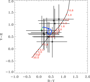
Figure 4. Color–color diagram for stellar-like counterparts. Squares: sources; solid black track: the Padova models for a zero-age main sequence for stars with solar abundances (Girardi et al. 2000), marked with their masses; blue track: the QSO track from z = 0 to z = 1. The green vector at the high-redshift end of the QSO track indicates the direction of motion in the diagram for AV = 0.1. The QSO spectrum is a combination of the optical spectrum from Vanden Berk et al. (2001), the IR spectrum from Glikman et al. (2006), and the UV spectrum from http://archive.stsci.edu/prepds/composite_quasar/ that was created from the spectra from Zheng et al. (1997).
Download figure:
Standard image High-resolution imageWe used the HST Hα images for two other classifications. Sources coincident with relatively regular Hα features that are disk-like or shell-like are likely to be young sources associated with Hα bubbles, H ii regions, or even SNRs. Such classification is somewhat dependent on the stretch applied to the Hα image; a rather regular feature may become quite irregular when lower surface brightness emission is included. In Table 6 we mark these as "HAB" (Hα blobs), while in the notes we have further characterized these sources as "filled," being relatively circular and having uniform or centrally peaked emission; "shell-like," having edge-brightened emission; or "irregular," having enhanced emission compared to the surroundings and distinct edges, but without being circular. Several of these sources are coincident with compact radio sources from Maddox et al. (2007), but we have not attributed these sources to SNRs; a separate study of the HST images taken in S ii will address that issue. This discussion is continued in the following section, where we discuss the Maddox et al. (2007) catalog.
We also note X-ray sources embedded in extended bright Hα emission where the X-ray source is not identifiable with any particular Hα substructure. The broadband images of these sources usually reveal bright, dense, often strongly confused stellar fields. These sources are labeled as "SFR," being in star-forming regions, and thus are more likely to be HMXBs or SNRs. There are also a number of sources that are projected against fainter diffuse Hα emission, but as it is not clear how to characterize these sources in any useful manner, we have not noted these cases in any particular way in Table 6.
Optical SDSS: For the region not covered by the HST images, primarily outside of the D25, the best optical material in hand is the SDSS. However, due to the brightness of M51, the SDSS photometry is limited to the outer part of our FOV, where the size of the Chandra PSF increases rapidly. Due to the somewhat poorer angular resolution of the SDSS compared to HST, classification of counterparts as either stellar or galactic is nontrivial. Thus, in the region with SDSS imaging but not SDSS photometry, we merely note the existence of optical sources within the Chandra PSF.
For sources within the region with SDSS photometry we list the SDSS source within the Chandra PSF that is closest to the source center. We have listed the SDSS classification for those sources with SDSS photometry. The SDSS source classes were assigned by comparing the source extension to the optical PSF (Stoughton et al. 2002), which will be least accurate for the faintest sources. The star−galaxy separation in the optical color–color–magnitude diagram is not strong even with the best selection of colors (u − g and g − r), so the SDSS extension-based classification cannot be reliably cross-checked using the photometry.
4.2. Comparison to Other Catalogs
Matching the sources in this Chandra catalog with sources in other catalogs can be problematic; the catalogs have been corrected to often unspecified coordinate reference frames and often do not record the astrometric uncertainties. Matching is particularly problematic when there is a high surface brightness of sources, so spurious matches are common. In most cases, source matching was done iteratively; two sources from different catalogs were deemed to be "matched" if one or the other falls within n times the positional uncertainty (where n has a value of 1–3), the mean (α, δ) offsets were calculated over all the matched pairs, and the offsets were then applied to one of the catalogs. This process is repeated until the set of matched sources does not vary and the remaining mean offsets are small, typically less than 10−4 arcsec.
The matching radius is generally set by the limitations of the Chandra astrometry. A measure of the uncertainty in the source positions can be obtained by comparing the source locations obtained from different observations after all of the observations have been corrected to the same coordinate frame. The mean offset between a source in a given observation and the mean location of that source is 035 at the center of our mosaic and becomes larger both with distance from the center and with faintness. By the D25 radius the positional uncertainty has not grown substantially, so we take a uniform criterion of 10 for matching sources to the X-ray catalog.
Historical Supernovae: The Asiago SN catalog (Barbon et al. 1999, and its dynamic online version) lists four SNe projected against the D25 of M51: 1945A (Kowal & Sargent 1971), 1994I (Puckett et al. 1994), 2005CS (Muendlein et al. 2005), and 2011DH (Arcavi et al. 2011, and references therein).
SN 1945A was not well studied but appears to have been of Type Ia. It is projected against the bright diffuse X-ray emission of NGC 5195, though it remains within the D25 of NGC 5194. There is no X-ray counterpart visible in the data.
SN 1994I was a Type Ibc, which was first detected in X-rays 6 yr after the explosion by Immler et al. (2002). The X-ray flux has declined as t−1.5 in recent years. It is projected to within ∼23'' of the nucleus, and while the background diffuse emission is strong, there is an X-ray counterpart easily seen 0798 from the SN position. Source X237 is relatively soft; it does not appear to have significant emission over 2 keV and (M−S)/T = −0.75 ± 0.23, (H−M)/T = −0.11 ± 0.16 (see Section 5.1 for a discussion of the colors). However, this source is quite close to another soft source, X242, so the photometry may be problematic. This source has been discussed by Rampadarath et al. (2015), using all of the Chandra data.
SN 2011DH was a Type IIb SN and was detected almost immediately in X-rays as reported in a detailed study by Soderberg et al. (2012). It is projected onto a spiral arm ∼26 southwest of the nucleus; it is nearly coincident with X369, having an offset of only 0632. The source has colors consistent with an absorbed thermal source, with (M−S)/T = −0.48 ± 0.04 and (H−M)/T = −0.14 ± 0.03. However, these colors could also be consistent with an only lightly absorbed high-index (Γ > 2) power-law source. The source was not detected before epoch D, declined from epoch D to epoch E, and showed no significant variation within the observations of epoch E. (See Table 2 for epoch definitions.) Thus, while the source is variable, the variability is not inconsistent with a young supernova. The X-ray properties have been discussed in detail by Maeda et al. (2014) using all of the Chandra data acquired since that time. They find that the X-ray spectrum can be characterized in terms of a two-temperature plasma from a hydrogen-deficient plasma.
SN 2005CS was a low-luminosity Type II plateau event with a low expansion velocity (∼1000 km s−1) (Pastorello et al. 2009), which was not detected with Swift in X-rays at the time (Brown et al. 2007), but the limits are not particularly restrictive. The SN is projected onto a spiral arm ∼11 south of the nucleus, and there is no X-ray counterpart visible in the data. Rampadarath et al. (2015) claim that there are two soft sources within 1'' of SN 2005CS, but neither of these sources appears in our X-ray catalog. The diffuse emission in this region is irregular, but none of the peaks are sufficiently significant to be considered sources.
Thus, of the four historical SNe, two have X-ray counterparts, while the other are below our detection limit.
Radio IDs: We matched our X-ray catalog to the FIRST catalog (White et al. 1997). After blind matching, we examined the FIRST images and discovered that a number of the FIRST sources to which X-ray sources were matched were extended and had poorly determined positions. In the nuclear region there were a number of spurious matches that we discarded. The FIRST position of the source near X163 does not match the object in the FIRST images, but the object in the image does match the X-ray source, so it was included despite having an offset larger than the tolerance. Source X415, for example, does not correspond to any FIRST catalog source, but happens to lie directly between two FIRST sources that form a single double-lobed source in the image.
We have compared our X-ray catalog to the radio catalog in Maddox et al. (2007) and find 42 matches, 13 of which were matched to Chandra sources in Maddox et al. (2007). The higher matching rate here is due primarily to a greater detection depth, but we do note that six of our sources that match sources in the Maddox et al. (2007) catalog are also matched to sources in the Kilgard et al. (2005) catalog, which suggests that the larger number of counts per source in this study has improved the measured source locations. Of the 47 matches, 40 are projected onto M51.
Clusters: Matching our X-ray catalog to the Hwang & Lee (2008) catalog derived from HST images is not trivial due to the high surface density of sources and mutual correlation of both X-ray sources and star clusters with star formation regions, which can produce a large number of spurious matches. Vulic et al. (2013) aligned the Chandra catalog to the 2MASS catalog using six reference sources. Given the dispersion in the offsets, this alignment seems rather uncertain. They also aligned the HST images to the 2MASS frame using a large number of sources and aligned the Hwang & Lee (2008) catalog to the HST images, from which it had originally been created.
We visually aligned the cluster catalog to the HST images, which allows an alignment to roughly an ACS pixel. The offset is large, the catalog coordinates being +0015 in R.A. and +055 in decl. compared to the HST images. Given that the bulk of the clusters lie within 30 of the center of the galaxy, where the PSF size is typically less than 5'', the PSF centroiding should be good to much better than an ACIS pixel (0492). We found 23 clusters lying within 1'' of a Chandra source. However, using the same type of analysis used in Kuntz et al. (2008), we found that 21 of those matches are likely to be spurious. Thus, we do not find it useful to identify those X-ray sources with coordinates matching those of clusters.
4.3. Summary of Identifications
Of the 298 sources within the D25, we find 13 background galaxies, 5 foreground stars, 6 stellar sources (possibly M51 globular clusters or background QSO), 50 Hα bubbles, and 18 sources embedded in large, confused star formation regions. Excluding sources embedded in star-forming regions, we have identified roughly one-quarter of the sources within the D25. Outside of the D25 we have identified three foreground stars and six background galaxies, or roughly 4% of the sources. We are unlikely to be missing any significant foreground stars, as foreground stars are distinctive in the HST data.
An Object of Particular Interest: X286 is roughly coincident (10) with an Hα source that is at the center of a large Hα shell. The shell is only partial, as if it is missing its polar caps, and has a radius of ∼19. This source is on the periphery of the galaxy and so would have expanded into a relatively low density environment. Although there is other diffuse Hα emission in this region, there are no clear signs of recently active star-forming regions.
5. DERIVED SOURCE CHARACTERISTICS
One of the prime foci of X-ray studies of nearby galaxies has been the luminosity function of populations of X-ray binaries. In order to construct the luminosity function of the binaries, one must identify and remove from the sample all of the point-like sources that are not X-ray binaries. In the case of M83 (Long et al. 2014), we identified foreground stars directly, identified the X-ray sources with optically and/or radio-identified SNRs, and removed the contribution of background active galactic nuclei (AGNs) statistically. We also noted that the SNR removal was likely to be incomplete as there is a population of faint soft X-ray sources whose composite spectrum was SNR-like, but lacking their (presumably) faint optical counterparts. For M51 we do not yet have sufficient data to identify and remove even the bright SNRs. However, using hardness ratio criteria and other supporting evidence, we can place interesting limits on the contribution of SNRs to the luminosity function. For this reason we will first consider the hardness ratios, color–color diagrams, and local source densities before proceeding to the luminosity functions.
5.1. Color–Color Diagrams
We use two normalized hardness ratios for color–color diagrams: (H−M)/T or [(2.6–8.0 keV)–(1.1–2.6 keV)]/(0.35–8.0 keV), and (M−S)/T or [(1.1–2.6 keV)–(0.35–1.1 keV)]/(0.35–8.0 keV). The left panel of Figure 5 shows the two hardness ratios for all of the significant sources, with 1σ error bars. The right panel of the same figure shows the regions of the diagram that should contain sources with typical spectral shapes: power laws and thermal spectra with different degrees of absorption. Either the bulk of the sources fall within those regions, or their 1σ error bars do. There are two regions with particularly high density of sources. The first is the relatively weakly absorbed thermal region. The second is a band running from unabsorbed power laws with indices >1.5 to absorbed (NH < 1021.5 cm−2) power laws with indices ∼1.5. The two regions are relatively well separated at (M−S)/T = −0.6.
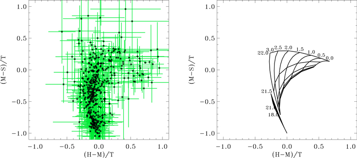
Figure 5. Left: color–color diagram for all sources, plotted with error bars. Right: grids showing the location of sources with different spectral shapes in the color–color diagram. The upper fan-shaped grid with labels is the grid for power-law sources, with the index running from right to left, and the log of the absorbing column density decreasing toward the bottom. The lower grid is the grid for thermal sources, with the log of the absorbing column density decreasing toward the bottom. The spread due to kT is very small for this choice of bands. The grids were calculated for chip S3 for ObsID 15553. Grids for different observations or different chips will vary, mostly in (M–S)/T, by less than ∼0.1.
Download figure:
Standard image High-resolution imageAs one might expect, highly absorbed thermal sources are nearly indistinguishable from more weakly absorbed high-index power laws. From what is generally known of SNRs, and from what was learned in M83, although many SNR sources will fall within the thermal region, not all X-ray sources associated with SNRs will be in the thermal region. Similarly, not all sources in the thermal region are SNRs as there are legitimate supersoft sources with similar colors.
The source types, from the identifications described in Section 4, are plotted in Figure 6.
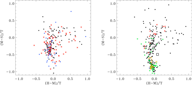
Figure 6. Left: color–color diagram for sources outside the D25 of the two galaxies. The blue crosses are sources identified as foreground stars, while the red crosses are sources identified as background galaxies. Right: color–color diagram for sources within the D25 for the two galaxies where the sources are coded by source type. Small black squares have not been identified, blue crosses are foreground stars and "stellar" sources, red crosses are galaxies, green diamonds are Hα blobs, orange squares are sources in large star-forming regions, and large black squares are the nuclei of the two galaxies.
Download figure:
Standard image High-resolution imageSources exterior to the D25: Although the sources outside the D25 are not the focus of this work, examination of the color–color diagram is of interest. The left panel of Figure 6 shows the sources outside of the D25 marked by type (foreground star, background galaxy, or unknown). The bulk of the stars are concentrated in the softest part of the diagram, though there is significant scatter. The background galaxies are distributed throughout the power-law region, but with sufficient scatter that it is clear that no classification can be made just from their location in the color–color diagram. Since the bulk of these sources are at the periphery of our FOV, the PSFs are large and the exposure times are low, and thus these sources have relatively poorly characterized hardness ratios. As noted above, there are significant uncertainties associated with the SDSS source classification. Thus, the scatter of source types within this diagram precludes the use of the color–color diagram from classifying any but the brightest of these sources.
Sources interior to the D25: The source types within the D25, which have higher total exposures and smaller PSFs, are mostly distributed in the manner that one might expect. The background galaxies are found in the power-law region with Γ ≳ 1.0 and are moderately to strongly absorbed. Sources with Hα counterparts fall in both the thermal region (and thus good SNR candidates) and the power-law region (and thus good HMXB candidates). Surprisingly, all the sources associated with extended, complex, and large star-forming regions are almost exclusively in the thermal region of the diagram, suggesting that many of those sources are either SNRs or compact diffuse emission regions (at a distance of 7.6 Mpc, 10 corresponds to 36.8 pc). There are a large number of uncategorized sources in the thermal region that may be either SNR candidates or extremely soft binaries. Of these sources, 24 have radio counterparts from Maddox et al. (2007).
Two of the sources identified as foreground stars are in the thermal region, as expected. There are two "stellar" objects that are in the power-law section of the diagrams. These are X081 ((M−S)/T = −0.089) and X095 ((M−S)/T = −0.212), which have stellar colors, but may be globular clusters in M51.
Very Soft Sources: Since the diffuse disk emission against which the sources are seen has (M−S)/T ∼ −0.92, it is quite possible that the very soft sources may include fluctuations in the diffuse emission that have angular sizes similar to the local PSF. If we define the very soft sources in much the same way as Di Stefano et al. (2004), −0.88 > (M−S)/T, we can check this possibility by comparing the composite spectrum of these sources with the mean spectrum of the diffuse emission. The spectrum is shown in Figure 7, where it is compared to the mean spectrum of the diffuse emission.
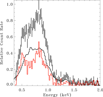
Figure 7. Composite spectrum of the very soft sources (−0.88 > (M–S)/T, error bars), compared to the spectrum of the diffuse emission (black histogram) normalized so that it does not exceed the source spectrum between 0.4 and 1.4 keV. The difference is shown in red.
Download figure:
Standard image High-resolution imageThe spectrum of the diffuse emission was extracted from the D25 region of NGC 5194, excluding point sources and excluding the inner r < 08 nuclear region. The particle background was constructed as described in Kuntz & Snowden (2010) and subtracted. This spectrum does contain some contribution from faint unresolved sources. However, given the very small flux at E > 2.5 keV, that contribution is small unless the unresolved sources have a spectrum that is significantly softer than the resolved sources. The spectrum of the diffuse emission has been scaled so that it does not exceed that of the sources anywhere in the 0.4–1.4 keV window, that is, it is scaled for the maximum possible contribution due to the diffuse emission.
Under this constraint, roughly 55% of the very soft source emission might be due to diffuse emission. Sources harder than −0.88 ∼ (M−S)/T are unlikely to be due to the diffuse emission simply due to their hardness.
5.2. Source Distribution
Figure 8 shows the source surface density as a function of the distance from the center of the arms for all of the sources within the D25 radius of NGC 5194 that are not projected onto the D25 region of NGC 5195. As one might expect, the source surface density increases strongly toward the center of the arm. Although the peak is offset slightly to positive values, a Kolmogorov–Smirnov test does not find any significant difference between the distributions on the positive and negative sides. Since for most of their length the arms are ∼07 apart, the decline in the surface density of sources at distances >07 is to be expected, simply because the only regions greater than that distance from an arm are just inside the D25 radius. The inner core of the distribution has a width of ∼05, which is roughly the width of the molecular arms. This concentration must not be taken as an argument that the X-ray source population is young since, if the arms are strong density waves, even the older populations will be concentrated there. This effect is demonstrated by the K-band distribution, which should trace the light of the old stellar population. The width of the full distribution of surface density of X-ray sources is comparable to the width of the distribution of the K-band light. There is a weak tendency for the sources in the arms to be softer (more negative in the (M−S)/T hardness ratio) than the sources farther from the arms, which suggests that the SNRs are more concentrated near the spiral arms.
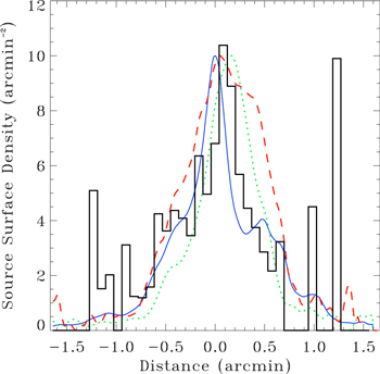
Figure 8. Solid histogram: source surface density as a function of the distance from the center of the spiral arms for sources within the D25 radius of NGC 5194, and not including sources projected against NGC 5195. No luminosity cuts were made for this figure as the point-source detection limit is not a strong function of the distance from the arm center. Positive values are on the inside of the arm. Dotted green line: CO distribution across the arm from the Heracles survey, normalized to an arbitrary value. Dashed red line: far-UV distribution across the arm from the GALEX images, normalized to an arbitrary value. Thin solid blue line: K-band distribution across the arm from 2MASS, normalized to an arbitrary value.
Download figure:
Standard image High-resolution image5.3. Variable and Transient Sources
Epoch-to-epoch or long-term variation: The opus of Chandra observations of M51 samples five separate epochs, beginning shortly after launch and continuing through the current epoch, covering 12 yr (see Table 2). The separations of the epochs of observations are, sequentially, 1 yr, 2 yr, 8 yr, and 1 yr. This spacing allows study of the long-term variation. We have used a common measure of variability:
where Fi is the measured photon flux at a given epoch and  is its uncertainty (Fridriksson et al. 2008). Rmax is the maximum Rij measured over all pairs of observations, i, j. We followed the procedure of Long et al. (2014): for each source we compare the measured Rmax with the distribution of Rmax created from 106 Monte Carlo simulations of observations of a constant source with the same mean flux, observation times, instrument response, and background regions as the observed source. We have labeled as variable any source for which the measured Rmax is greater than 99.73% (i.e., 3σ) of the simulated Rmax. The left panel of Figure 9 shows the fractional amplitude of the variation (Rmax/2Fmean, where Fmean is the mean flux for the source determined over all observations) that could be detected for each source in the 0.35–8.0 keV band. Of the sources within the D25 radius, roughly 24% (72) were found to be variable.
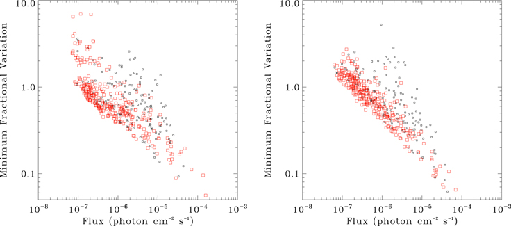
Figure 9. Left: smallest fractional variation (Rmax/2Fmean) detectable for each source as a function of the source flux in the 0.35–8.0 keV band. The red points are sources within the D25 regions, and the black points are the remainder of the sources. Right: same as the left panel, but for the seven epoch E observations taken in 2012 September/October.
Download figure:
Standard image High-resolution imageObservation-to-observation or medium-term variation: Given the large amount of exposure spread over the seven observations of epoch E in 2012 September/October, we can also measure a "medium-term variability" in the same manner over the month required to obtain the new observations. The right panel of Figure 9 shows the amplitude of the variation that could be detected for each source in the 0.35–8.0 keV band. Of the sources within the D25 radius, 28 were found to be variable in both the long-term and medium-term; 34 were found to be variable in the long-term, of which 21 should have been detected in the medium-term at the same amplitude of variation; and 8 were found to be variable only in the medium-term, of which 2 should have been detected in the long-term at the same amplitude of variation. Thus, it would appear that roughly half of the sources with long-term variability also show medium-term variability, while very few sources with medium-term variability do not also show long-term variability.
Variable Sources in the color–color diagrams: As can be seen in Figure 10, the variable sources are distributed predominantly in the power-law portion of the color–color diagram, although there are several in the soft, predominantly thermal portion of the diagram. Thus, the difference in hardness ratios between the variable sources and those not detected as variable is larger for the (M−S)/B ratio than for the (H−M)/T ratio. The variable sources have (M−S)/T = −0.158 ± 0.037, while the remainder of the sources have (M−S)/T = −0.349 ± 0.016. The variable sources have (H−M)/T = −0.034 ± 0.015, while the remainder have (H−M)/T = 0.006 ± 0.011. This result is consistent with the softest sources being dominated by SNRs and/or unresolved diffuse emission, which would not be variable.
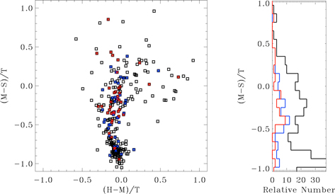
Figure 10. Left: color–color diagram for sources within the D25. Blue symbols mark sources with long-term variation, that is, the variation from one observation epoch to another. Red symbols mark sources with medium-term variation, that is, the variation from one observation to another during the 2012 observations. Right: histogram of the hardness ratios of all sources (black), sources with long-term variation (blue), and sources with medium-term variation (red).
Download figure:
Standard image High-resolution imageOf the soft sources (92 with −0.55 > (M−S)/T > 0.88) that might be SNRs, only 13 have detected variability. Of the very soft sources (29 with −0.88 > (M−S)/T) that might also be SNRs, only 2 have detected variability. Thus, very few of the SNR candidates identified from X-ray colors can be eliminated through variability.
Transients: Of the variable sources, transients are of particular interest as they trace a particular population of black hole binaries that can be compared to that observed in the Milky Way. We define transient sources to be those variable sources with Rmax > 4, and most observations are low or consistent with zero. As there is some dispersion in the definition of a "transient," we have further categorized the transients as follows. Classical transients (12 instances) have only one high measurement, and the remainder of the observations are consistent with zero. Bursters or repeating transients (three instances) have two nonconsecutive high measurements, while the remainder of the observations are consistent with zero. Nontraditional transients (four instances) have either one or two high measurements, while the remainder of the observations are not consistent with zero, but are a factor of 4 or more below the high measurements. These might be detected as transients had the galaxy been a bit farther away.
We should also note that two sources (X302, X175) dimmed and became nearly undetectable over these observations, while one source (X188), which was undetected in the first three observations, increased its brightness over the final two. These sources are of interest because they demonstrate either smooth long-term variation or further candidate repeating transients (such as M101 ULX-1). One further source (X369) was undetected in the first three epochs, as discussed under historical supernovae. Finally, we note three sources (X376, X396, and X107) with relatively constant fluxes but a single observation for which the flux was strongly diminished. These "dropout" sources might be eclipsing binaries serendipitously caught, but the eclipses would have to be 7–14 hr long, implying a wide separation.
5.4. Luminosity Function
Given that there are two overlapping galaxies within the FOV, the issue of the luminosity function becomes somewhat more complicated. We will first discuss the luminosity function for the region covered by the two D25, before considering the separation of the luminosity functions.
The left panel of Figure 11 shows the progressive isolation of the 0.5–2.0 keV luminosity function of sources within M51. The solid black histogram is the raw luminosity function of all the sources projected against the disks of M51. The dashed red line is the expected contribution from background AGNs, calculated for the same region from which the luminosity function was taken. The assumed flux function of the background AGNs was taken from Kim et al. (2007) and was corrected for the point-source detection limit and galactic absorption on a 0492 × 0492 pixel-by-pixel basis. The luminosity function for the identified background galaxies is given by the dashed black histogram. Due to both the optical brightness of M51 and its absorption, the luminosity function for the identified background galaxies is a significant underestimate of the expected AGN function. The raw luminosity function after the subtraction of the expected AGN function is shown by the solid red histogram. We further removed the foreground stars (dashed green histogram) to yield the luminosity function for sources in M51 (solid green histogram). The lower limit to the luminosity function, slightly below 1036 erg s−1, was taken to be the luminosity at which the correction factor was less than 20%. That is, the point-source detection limit is lower than that luminosity over 80% of the area. We construct luminosity functions for several different regions; in all cases the correction factor has been computed for the region of interest, and the correction factor has been applied before the luminosity function is plotted. Since the point-source detection limit varies with location, the depth of the luminosity function depends on the region over which it is formed.
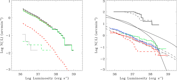
Figure 11. Left: 0.5–2.0 keV band cumulative luminosity function (in sources per arcmin−2 brighter than some luminosity) for sources within the D25 of the two galaxies. Black histogram: the total luminosity function; dashed red histogram: the extragalactic flux function scaled to the distance of M51; solid red histogram: the luminosity function from which the AGN has been subtracted; dashed green histogram: the foreground stars; solid green histogram: the luminosity function from which the AGN and foreground stars have been subtracted. Right: the cumulative luminosity functions for different regions. Black histogram: the nuclear region of NGC 5194 (R < 12''); dashed black histogram: the inner 45'' of NGC 5195 (shifted upward by 1 in  ); blue histogram: the disk of NGC 5194 where it does not overlap the disk of NGC 5195; green histogram: the region of overlap between NGC 5194 and NGC 5195 (there are too few sources within the D25 of NGC 5195 that are not in the overlap region to plot); dotted black histogram: the sum of the NGC 5194 "disk-only" luminosity function and that of the overlap region; dashed red histogram: the soft sources (those with (M–S)/T ≤ −0.55) of the disk of NGC 5194 alone; solid red histogram: the disk of NGC 5194 after the removal of the soft sources; solid black curves: the Grimm and Gilfanov curves for HMXB and LMXB luminosity functions with arbitrary normalizations; dashed black curves: the Grimm curve for HMXB with normalizations of 1.6 and 2.5 M☉ yr−1.
Download figure:
Standard image High-resolution imageThe right panel of Figure 11 shows the cumulative luminosity functions for different regions of M51. The nuclear region of NGC 5194, the inner 12'', is the region in which there is the greatest confusion by bright, structured diffuse emission. As a result, the luminosity function for this region is likely to be incomplete at fluxes above the formal completion limit. The luminosity function (black histogram) is roughly flat below  , where it has a break, and then appears to have a second sharper downward break at
  , and, finally, it has a much shallower slope above
  . The shape of the nuclear luminosity function is vaguely reminiscent of the classic Gilfanov (2004) LMXB function. Although the luminosity of the first break is similar to that found by Gilfanov (2004) (2 × 1037 erg s−1 in 0.3–8.0 keV = 7 × 1036 erg s−1, depending on the assumed spectral shape), the rollover is far too sharp for the Gilfanov (2004) LMXB function. However, given that this region contains only 14 sources significant in the 0.5–2.0 keV band, the disagreement may not be significant.
The luminosity function for the disk of NGC 5194 that is not projected against NGC 5195 (NGC 5194 "disk-only") is shown by the blue histogram in the right panel of Figure 11. It is well described by a power law of α ∼ 1.7 from  to
to  , slightly steeper than the classic Grimm et al. (2003) HMXB function (α ∼ 1.61). Here we follow the convention of giving the slope of the differential luminosity function (N(L) ∝ L−αdL) while displaying the cumulative luminosity functions (N(>L) ∝ L1−α). There are too few sources in the portion of the disk of NGC 5195 that does not overlap NGC 5194 to form a luminosity function. The luminosity function of the overlap region is fairly flat below
  (α ∼ 0.3) and becomes steeper at higher luminosities. Since roughly half of the sources in the overlap region appear to be clustered around the core of NGC 5195 and the remainder are NGC 5194 disk sources, and since NGC 5195 has very little star formation, one might expect the luminosity function of the overlap region to combine the power law of the disk with an LMXB-like function. Indeed, this is the case. The luminosity function of the core of NGC 5195 (the inner 45'') is shown by the dashed black histogram in Figure 11, shifted upward by one order of magnitude. It shows a roll-off that is similar to that found in the nucleus of NGC 5194 in both magnitude and luminosity limits. Since the core of NGC 5195 provides only 12 sources in the overlap region, compared to the 231 sources in the NGC 5194-only region, the addition of the sources in the overlap region changes the NGC 5194 luminosity function only slightly (the dotted line in the right-hand panel of Figure 11), by decreasing the slope slightly.
It should be noted that the NGC 5194-only luminosity function is the luminosity function for sources in NGC 5194, but is not restricted to binaries alone since we do not yet have a catalog of SNRs. However, we can get a reasonable limit to the binary luminosity function without an SNR catalog. From our study of M83 (Long et al. 2014), we found that roughly half of the sources in the lightly absorbed thermal region of the color–color diagram were clearly SNRs, and there were indications that some fraction of the sources in that region of the color–color diagram that were not identified as SNRs in the optical or radio were also SNRs. Thus, if we assume that all of the sources in that region of the color–color diagram are SNRs, we can then obtain a lower limit to the binary luminosity function; the luminosity function without the SNR removal forms the upper limit to the binary luminosity function.
In the right-hand panel of Figure 11 the dashed red line shows the luminosity function of sources with (M−S)/T < −0.55, which effectively selects the sources in the unabsorbed thermal region of the color–color diagram. We have assumed that these soft sources will not contain a significant contribution from AGNs. Clearly, this luminosity function must contain some binaries, as SNRs with  are unlikely. Ignoring these few very bright sources, the remainder of the luminosity function has much the same shape as the SNR luminosity function in M83, with an effective cutoff of
  . Once this limiting SNR luminosity function is removed from the NGC 5194 disk-only luminosity function (the solid red histogram in the right-hand panel of Figure 11), the remainder is still well characterized by a power law with α ∼ 1.55. There is a tendency for the luminosity function to flatten a bit at the lowest luminosities, which is the portion of the luminosity function with the largest corrections.
Using both of these limits to the binary luminosity function, we see that the binary luminosity function must be characterized by a power law with an α between 1.55 and 1.7. Our upper limit is consistent with the value found by Kilgard et al. (2005), which could not be corrected for SNRs. Thus, following the Grimm et al. (2003) characterization of the luminosity function, the NGC 5194 disk binary luminosity function is likely dominated by HMXBs. Comparing the normalization of this luminosity function (following the blue histogram in Figure 11) to the Grimm et al. (2003) luminosity function, we find a star formation rate of 2.5 M☉ yr−1, similar to the measured current star formation rate of 2.7 M☉ yr−1. This agreement is not unexpected since Grimm et al. (2003) used the early M51 Chandra data to calibrate the HMXB function. It is to be noted that the luminosity function to which we have compared includes the SNRs, as did the data from which Grimm et al. (2003) originally derived the HMXB luminosity function.
6. THE NUCLEUS
X-ray emission from the nuclear region of NGC 5194, particularly the inner 025, is a complex mixture of resolved sources, strong diffuse soft emission, and unresolved sources (see Figure 12). Reliable detection and characterization of point sources in such a region is difficult. In this region the combination of wavdetect detection and AE photometry produced a list of >20 statistically significant sources. Of those, the six sources detected at E > 2.0 keV are (mostly) free from confusion and could be in/excluded on the basis of the statistics within the hard energy band. Sources detected only at E < 2.0 keV, however, were problematic. Several were strongly overlapping or strongly irregular, and all were in regions with strong, highly structured diffuse emission features. Since the background structure has a surface brightness comparable to the sources and has variation on the scale of the PSF, the values required for statistical methods for determining the significance of sources are poorly defined. Spectral characterization was also insufficient to separate candidate sources from the background; none of the soft sources had spectral features significantly different from those of the pseudo-diffuse background.
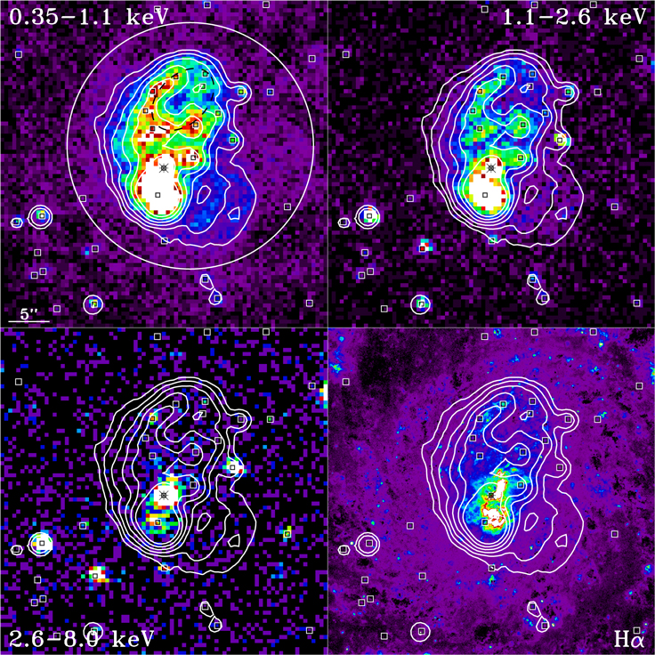
Figure 12. Images of the nuclear region of NGC 5194. The countours are taken from the 350–1100 eV image after smoothing by a 25 top hat function. The squares indicate significant sources from the catalog. The circle has a radius of 025 and delineates the region that has significant structured diffuse emission. The asterisk marks the nominal nuclear source. The dashed ellipse is the location of the "Northern Bubble."
Download figure:
Standard image High-resolution imageFor these reasons, we were forced to use rather less objective criteria for sources identified only at E < 2.0 keV. Several of these sources appeared to be multiple offset detections of the same source, and although we cannot rule out these sources being the aggregate of a number of variable sources, we removed what we judged to be duplicate detections. After removing these duplicate sources, we ran AE again, allowing AE to determine and refine the source locations, and retained sources deemed by AE to be significant. Thus, sources identified only at E < 2.0 keV may not be true point sources, but may be peaks in the diffuse emission, so the catalog of soft sources within 02 of the nucleus should be approached with caution.
Figure 12 shows the locations of the 17 sources that were accepted as significant. The partial ring of X-ray emission, marked in the figure with a dashed ellipse, is closely related to the northern ring observed in the radio (Terashima & Wilson 2001). Several sources lie on the shell of the northern ring and may be knots of diffuse emission. The brightest part of this ellipse had a high density of seemingly duplicate sources, and reference to the wavdetect runs for individual ObsIDs shows a large variation in the measured source locations. Thus, the characterization of the sources in this arc is not certain. The northern ring is partially traced by Hα emission, but the strength of the Hα emission is not correlated with the strength of the X-ray emission.
Similarly, our source X211 is coincident with the radio-defined extra-nuclear cloud (XNC), and thus its emission is likely be dominated by diffuse emission. However, this source is more complex. Terashima & Wilson (2001) noted that the northeast part of the X-ray emission coincident with the XNC was harder than the remainder of the X-ray emission from the XNC and, arguing that this region was aligned with the jet axis defined by the location of the nucleus and the position angle of the optical/radio elongation, suggested that the hard emission represents the terminus of the jet. Our deeper exposure shows clearly extended hard emission surrounding the nominal position of source X211, as well as a concentration of hard emission ∼05 northeast of X211. Whether the concentration is the jet terminus or a point source superposed on a more extended emission region remains to be seen. The spectra from the concentration and extended emission are not significantly different. However, we note that our source X211 does show some variability among the 2012 observations, particularly in the soft band, which suggests a substantial contribution from a point source or jet terminus.
Our deeper exposure also reveals structures missed in earlier studies. To the west of the XNC, and roughly concentric with its boundary, are two X-ray emitting "filaments." These structures are clearly seen in the 0.35–1.1 keV band. Both can be seen in the 1.1–2.6 keV band, but only the brighter inner one can be seen as a filament; the outer one is merely a region of extended emission. Neither is apparent in the hardest band. The inner filament has a faint Hα counterpart. Considered as edge-brightened shells, these structures may be relict shells from previous outbursts.
7. DISCUSSION
7.1. M51 by Itself
It is well known that NGC 5194 has a strong density wave with a strong arm-interarm contrast. It is generally accepted that the companion is, at least in part, responsible for the strength of the density wave. Salo & Laurikainen (2000) showed that there is a broad range of encounter parameters that can produce the observed morphology and showed that the current spiral pattern formed independently of the pre-encounter disk morphology. Even in the case of a pre-encounter axisymmetric disk, a strong m = 2 pattern is produced within 200 Myr of the first encounter. The arms continue to be strong to the current day (∼500 Myr post-encounter) though significantly more tightly wrapped. In such a scenario, the original disk population (i.e., the population traced by the current LMXB) would be compressed into arms, where there is subsequent star formation. Thus, we expect for such a strong density wave as found in NGC 5194 that both young and old populations are to be found predominately in the arms as, indeed, they are.
A simple interpretation of Grimm et al. (2003) and Gilfanov (2004) would suggest that the X-ray binary population of M51 is dominated by HMXBs. Grimm et al. (2002) constructed luminosity functions of the X-ray binary populations in the Milky Way, showing that the HMXB cumulative luminosity function was well characterized as a power law with a slope of −0.64 ± 0.15 while the LMXB cumulative luminosity function was characterized by a cutoff power law with multiple breaks or strong curvature. The dichotomy was strengthened when Grimm et al. (2003) and Gilfanov (2004) created mean luminosity functions for galaxies with high and low star formation rates, and identifying the results as HMXB- and LMXB-dominated luminosity functions. It was suggested that these functions represented "universal" luminosity functions.
However, the interpretation of the power-law luminosity function in M51 as an HMXB-dominated luminosity function is not supported by what little we know of the star formation history of M51. The Salo & Laurikainen (2000) study suggested either a single pass by NGC 5195 some 500 Myr ago or repeated passages beginning at the same time, with the most recent pass 50–100 Myr ago. In the first case one might expect a single, perhaps rather extended burst of star formation as the disk was reorganized into the strong m = 2 pattern, some 300 Myr ago. The second case suggests multiple episodes of star formation corresponding to multiple close approaches. The star formation history derived from a study of stellar clusters (Hwang & Lee 2010) suggests a strong episode of star formation between ∼50 and ∼300 Myr ago with a short, relatively minor burst of star formation 5 Myr ago. These histories would suggest that the X-ray binary population in M51 is dominated by LMXBs.
For an instantaneous starburst the aggregate HMXB luminosity drops rapidly over the first 20 Myr, plateaus, and drops again after ∼50 Myr, crossing the rising aggregate LMXB luminosity somewhere around 75 Myr (Fragos et al. 2013; their function is shown in the top panel of Figure 13). The LMXB luminosity, in contrast, rises slowly over the first 1000 Myr and drops thereafter. Although the Fragos functions are in terms of luminosity rather than in the number of sources, it is clear that in less than 20 Myr after a starburst, the ratio of HMXB to LMXB luminosity is only ∼10, and unlikely to show the strong HMXB-dominated luminosity function. For continuous star formation, as shown in Figure 13, where we assume star formation for the last 500 Myr, HMXB/LMXB ∼ 10 after 70 Myr. Thus, the HMXB-dominated luminosity function in M51 is possibly consistent with a constant and elevated star formation rate since a last close passage 50 Myr ago. It is rather more easily consistent with a strong, more recent episode of star formation. However, the star formation history constructed from counting stellar clusters produces a large LMXB population from the 300 Myr to 50 Myr burst, but very few HMXBs from the very short recent burst. Even if the star formation rate over the last 10 Myr rivals the highest star formation rates in the past, the total HMXB luminosity will still be less than that of the LMXBs.
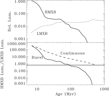
Figure 13. Top: relative X-ray luminosity of the HMXB and LMXB populations from Fragos et al. (2013). Bottom: ratio of the HMXB/LMXB luminosity as a function age for a single burst (solid) or continuous star formation (dashed). Note that the data presented in Fragos begin at ∼7 Myr after the star formation.
Download figure:
Standard image High-resolution image
The disagreement between our understanding of the M51 luminosity function and the Grimm and Gilfanov "universal" luminosity functions requires exploration. For the moment, we will assume that the power-law HMXB luminosity function is correct, and will examine the LMXB luminosity function instead. We first note that the Galactic LMXB luminosity function is extracted from a population with a constant to falling star formation rate over the last ∼10 Gyr (e.g., Boissier & Prantzos 1999), though this history may have been punctuated by bursts (Rocha-Pinto et al. 2000). The composite LMXB luminosity function constructed by Gilfanov (2004) used data from a variety of galaxy types with a variety of different star formation histories; the high end of the luminosity function is dominated by data from ellipticals and S0 galaxies, while the low end is dominated by M31 (presumably bulge fields) and the Milky Way. There is a discernible variation in the shape of the individual LMXB luminosity functions that were used to form the composite luminosity function.
Such a composite luminosity function would not be valid in the presence of significant evolution, e.g., a simple model such as that proposed by Wu (2001) and Kilgard et al. (2002). In these cases, the birth function was assumed to be a power law. If the lifetime is inversely proportional to the luminosity, there will be a break in the power law that, for an instantaneous starburst, moves to progressively lower luminosities with time. There is some evidence for such evolution: both Kim & Fabbiano (2010) and Zhang et al. (2012) showed that young ellipticals (<5 Gyr) have luminosity functions that extend to higher luminosities than older ellipticals (>5 Gyr), while having much less significant breaks. These studies suggest that young LMXB populations have power-law-like luminosity functions, with breaks that become stronger with age. We should also note that reality is much more complicated. For example, there are some old elliptical galaxies with no clear break up to the brightest source at ∼7 × 1038 erg s−1. The globular cluster LMXB population and the field LMXB population appear to have different luminosity functions, as we have been most recently been reminded by Lehmer et al. (2014). Thus, the true evolution of luminosity function with age is as yet unclear.
Given the variety of LMXB luminosity function shapes, from strongly curved to nearly pure power laws, "hiding" a substantial LMXB population within a luminosity function well described by an unbroken power law seems unproblematic. If indeed "young" (≲5 Gyr) LMXB populations tend to have minimal breaks as implied by Kim & Fabbiano (2010) and Zhang et al. (2012), then it is not unreasonable to expect the 0.3 Gyr old LMXBs to have a roughly power-law luminosity function. Careful application of population synthesis models should reveal whether this supposition is truly reasonable.
Since the star formation history suggests that the X-ray binary population in M51 contains a substantial fraction of LMXBs, and we can reasonably propose that the LMXBs have a power-law-like luminosity function, we must revisit the issue of the "universal" HMXB luminosity function. The differential Milky Way HMXB luminosity function has a slope of −1.64 ± 0.15 (Grimm et al. 2002). The differential composite HMXB luminosity function derived from a set of actively star-forming galaxies (including M51) has a slope of −1.61 ± 0.12. We have found that the M51 luminosity function has a differential luminosity function with a slope −1.7 < α < −1.55. The admixture of LMXBs in the M51 luminosity function does not seem to have produced a significantly different slope, which suggests that the true slope of the HMXB luminosity function, for a broad range of star formation histories, will be similar.
Mineo et al. (2012) has also constructed a composite HMXB luminosity function, using a much broader sample of vigorously star-forming galaxies. They attempted to correct the composite luminosity function for the contribution of LMXBs assuming the "universal" LMXB luminosity function and the Gilfanov (2004) scaling between the number of LMXBs and the stellar mass of the galaxies. They found that the resulting LMXB luminosity function had an amplitude that was greater than that of their measured luminosity function in the 1036.5–1038.5 erg s−1 range. They attribute this oversubtraction to two issues: that the Gilfanov (2004) scaling is taken primarily from elliptical galaxies rather than from star-forming spirals, and that the scaling relation for young populations of LMXBs appears to have lower normalization. We would further suggest that the LMXB luminosity function for the star-forming spirals may be significantly broader than the "universal" function, which would further reduce the problem. Mineo et al. (2012) also note a large scatter in the correlation between the normalization of the HMXB luminosity function and the star formation rate. Since different star formation histories will produce different HMXB/LMXB ratios for the same current star formation rate/stellar mass ratio, this scatter is not surprising.
Certainly, M51 demonstrates the inadvisability of presuming an HMXB-dominated population based on the shape of the luminosity function. This study also demonstrates the need to determine the detailed star formation history for M51, and the need for a population synthesis, before this seemingly simple system can be understood.
7.2. M51 in Comparison
There are a limited number of galaxies for which the luminosity function has been measured down to ∼1036 erg s−1. Of those, M83 is a close analog to M51. M83 has a star formation rate of 3.06 M☉ yr−1 (Jarrett et al. 2013, corrected from their assumed distance to 4.7 Mpc), an H i mass of 1.7 × 10⁹ M☉ (Walter et al. 2008), and a molecular mass of 3.9 × 10⁹ M☉ (Lundgren et al. 2004). The ratios of the luminosities of the two galaxies in the WISE bands dominated by the old stellar population, W1 and W2, are M83/M51 = 0.78 and 0.79 (Jarrett et al. 2013), meaning that M83 has a stellar mass that is ∼80% of that of M51. The ratio of the half-light radius (in physical units) is 0.77 (Jarrett et al. 2013), while the ratio of their D25 in physical units is 0.71, suggesting that the disk of M83 is somewhat smaller than that of M51, but not significantly so.
The differences between M51 and M83 include a slight difference in Hubble type (M83 is an SAB(s)c) and the nature of their starbursts. The M51 star formation is likely being triggered by the interaction between NGC 5194 and NGC 5195, with the star formation being well distributed throughout the disk. The M83 star formation is strong in the arms, but concentrated in the nucleus, perhaps due to M83 having a noticeable bar. Long et al. (2014) found the M83 luminosity function to be dominated by LMXBs, but with a significant admixture of HMXBs, perhaps suggesting that the recent starburst is adding a transient HMXB population to the existing population of LMXBs produced by relatively continuous star formation.
The number of sources within D25 to a limiting luminosity of 1036 erg s−1 in the 0.5–2.0 keV band (where the Chandra response is the strongest and is not strongly affected by the increasing low-energy absorption problem) is 231 for M51 (of which ∼34 are background AGNs) and 191 for M83 (of which ∼41 are background AGNs), for an M83/M51 ratio of 0.77, which is quite similar to the ratio of their stellar masses. The fraction of soft sources (−0.88 < (M−S)/T < −0.55) in M51 is 31%, while in M83 it is 28%. The fraction of very soft sources (−0.88 > (M−S)/T) in M51 is 9%, while in M83 it is 20%; this difference is likely due, at least in part, to the reduction in soft response between the M83 and the M51 observations.
Given the similarity of the stellar masses and the star formation rates, one would expect the two galaxies to have a similar number of X-ray sources. Of interest is the difference in the shapes of the luminosity functions; M83 has a (marginally) higher star formation rate, yet has a luminosity function that is not dominated by HMXBs, in that there is significant curvature in the luminosity function. Conversely, the M51 luminosity function is relatively well described by a single power law, despite a (marginally) lower star formation rate. This difference is, of course, to be expected; if NHMXB is the number of HMXBs,  is the fraction of HMXBs expected to emit a time t after star formation,
  is the star formation rate τ years ago, and f is the fraction of stars producing HMXBs, then

where τ is the look-back time to the birth of the system. Thus, we are reminded that the current HMXB population is due to star formation over the last 5–10 Myr, so it may not be entirely represented by the current star formation rate.
However, the point remains that M83 and M51 have different luminosity functions. Within the framework of the previous discussion, some component of M83 has a luminosity function that has one or more strong breaks, while M51 does not. Thus, one expects that the long-term star formation history of the two galaxies should be very different. Given that both of these galaxies are relatively nearby, more detailed histories and comparative population synthesis for these two galaxies should be illuminating.
8. SUMMARY
M51 contains a healthy population of X-ray sources, of which we have identified multiwavelength counterparts to roughly one-quarter of those detected. The bulk of the sources are concentrated in the spiral arms, in the same way that the bulk of the stellar population is concentrated in the spiral arms. The large number of sources in the thermal region of the color–color diagrams, the association of soft sources with Hα shells, and a slightly higher concentration of soft sources in the arms suggest that M51 will be found to contain a large number of SNRs, as might be expected from the vigourous star formation rate and the number of historical supernovae.
The 12 yr Chandra baseline provides an opportunity to study the variability of the source population. We found that roughly one-quarter of the sources varied between epochs (multiyear scales) and ∼15% varied over the course of the month in which our data were taken. Fifteen sources are clearly transient or bursters, and another four would fit the classical definition of a transient had our observations not been so deep. We have also found that the active ULX population in M51 seen in more recent observations is generally not as large as seen in the early Chandra observations. Given the strong variability of the sources that sometimes enter the ULX regime and the relatively small number of objects involved, this difference is not surprising.
By removing the background AGNs and foreground stars from the luminosity function of the disk of NGC 5194, we obtained the luminosity function of the sources in the disk. Since this curve includes the SNRs, it is an upper limit to the binary luminosity function. Based on our experience with M83, we used a "best guess" of the SNR luminosity function to derive a lower limit to the binary luminosity function. Both limits have a slope similar to that of the canonical HMXB luminosity function, suggesting that the disk of NGC 5194 is dominated by young binaries. The star formation rate derived from the luminosity function agrees with the star formation rate derived from IR and UV measurements. However, the star formation history derived from stellar clusters indicates that the luminosity function should be dominated by LMXBs, not HMXBs. Conversely, if the luminosity function is dominated by LMXBs, then our understanding of a "universal" LMXB luminosity function will need to be revised.
Support for this work was provided by the National Aeronautics and Space Administration through Chandra grant number GO-213103A, issued by the Chandra X-ray Observatory Center, which is operated by the Smithsonian Astrophysical Observatory for and on behalf of NASA under contract NAS8-03060. This work was also supported by the National Aeronautics and Space Administration through HST grant number GO-12762.007 issued by the Space Telescope Science Institute. We thank Derek Hammer for producing the HST images used here. Finally, we must thank the referee for pointing out a number of places where we needed to make the commentary more pointed.
Facilities: Chandra (ACIS) - , HST (ACS). - Hubble Space Telescope satellite
Footnotes
- ∗
Based on observations made with NASA's Chandra X-ray Observatory, which is operated by the Smithsonian Astrophysical Observatory under contract #NAS83060, and the data were obtained through program GO1-12115.
- 5
We will use M51 to refer to the pair of galaxies, while we will use the NGC numbers to refer to the individual members of the pair.
- 6
For completeness, we note that as part of our study of X-ray sources in M51, we used HST/WFC3 to acquire narrowband [S ii] images of four fields in M51 (Proposal ID 12862, PI: K.D. Kuntz). The [S ii] images will be used as part of a future publication in an effort to identify the SNRs in M51, and to study both their optical and X-ray properties. In this report, we use only the broadband and Hα images from the Legacy Project.
- 7