


Abstract
The β-delayed neutron-emission probabilities of 28 exotic neutron-rich isotopes of Pm, Sm, Eu, and Gd were measured for the first time at RIKEN Nishina Center using the Advanced Implantation Detector Array (AIDA) and the BRIKEN neutron detector array. The existing β-decay half-life (T1/2) database was significantly increased toward more neutron-rich isotopes, and uncertainties for previously measured values were decreased. The new data not only constrain the theoretical predictions of half-lives and β-delayed neutron-emission probabilities, but also allow for probing the mechanisms of formation of the high-mass wing of the rare-earth peak located at A ≈ 160 in the r-process abundance distribution through astrophysical reaction network calculations. An uncertainty quantification of the calculated abundance patterns with the new data shows a reduction of the uncertainty in the rare-earth peak region. The newly introduced variance-based sensitivity analysis method offers valuable insight into the influence of important nuclear physics inputs on the calculated abundance patterns. The analysis has identified the half-lives of 168Sm and of several gadolinium isotopes as some of the key variables among the current experimental data to understand the remaining abundance uncertainty at A = 167–172.
Export citation and abstract BibTeX RIS

Original content from this work may be used under the terms of the Creative Commons Attribution 4.0 licence. Any further distribution of this work must maintain attribution to the author(s) and the title of the work, journal citation and DOI.
1. Introduction
About half of the elemental abundances heavier than iron are the result of the rapid neutron capture process (r-process) in which neutron capture, β-decay, and many other reactions occur over a timescale of seconds (Burbidge et al. 1957; Cameron 1957; Cowan et al. 2021). This process requires high neutron densities in excess of 1020 neutrons/cm3 in explosive stellar environments. Accordingly, for a long time, the two favorite candidates have been core-collapse supernovae (CCSN) and neutron-star mergers (for a review, see Cowan et al. 2021).
Observations of galactic halo stars have revealed that the abundance patterns of heavy (A ≥ 56) elements show consistent signatures of the solar system r-process abundances (Cowan & Sneden 2006). This suggests that these old stars were polluted by prior r-process events in which the heavy element abundance pattern is robustly reproduced. Moreover, spectroscopic studies of the oldest stars in our galaxy and in neighboring dwarf galaxies (see, e.g., Reichert et al. 2020) suggest that the r-process must have occurred before neutron-star mergers would have been able to contribute significantly to the observed abundances. These observations mean that CCSN are one possible site of the r-process. Recent work showed that magnetorotational supernovae are able to synthesize a sufficient amount of heavy elements (Winteler et al. 2012; Mösta et al. 2018; Siegel et al. 2019; Yong et al. 2021).
On the other hand, the detection of the gravitational wave signal GW170817 triggered by a binary neutron-star merger event by the LIGO/Virgo detectors allowed performing detailed observation of its electromagnetic counterpart AT2017gfo (Abbott et al. 2017a, 2017b). The light curve of this event (kilonova), powered by the radioactive decays of exotic neutron-rich nuclei, provided the first direct evidence for the occurrence of the r-process in a neutron-star merger (Kasen et al. 2017). However, to fully understand these observations and r-process nucleosynthesis, much more detailed nuclear physics information is needed.
The main signature of the solar r-process abundance distribution are two large abundance peaks, located at A ≈ 130 and A ≈ 195, which originate from the increased stability at the neutron shell closures N = 82 and N = 126. A smaller abundance peak exists in between these two peaks around A ≈ 160, which is known as the "rare-earth peak" (REP). Since this small abundance peak is located in between the neutron shell closures, other mechanisms must play a key role in synthesizing these isotopes.
Indeed, while the two main peaks form during the (n, γ) ↔ (γ, n) equilibrium, the REP takes shape in later phases of the r-process after the temperature and the density of available neutrons significantly drop and the material starts to decay back to stability (freeze-out). According to this picture, understanding the synthesis of the lanthanides in this mass region may allow us to probe the detailed conditions of the freeze-out and the mechanisms of the r-process that robustly reproduce the abundance pattern occurring in stars over a wide range of metallicities (Surman et al. 1997; Mumpower et al. 2012).
The formation of the REP is sensitive to variables that control the neutron density and neutron-to-seed ratio in the late stages of the r-process, such as the timescale for the expansion of the material. However, these astrophysical conditions are entangled with nuclear physics processes that provide additional neutrons, of which β-delayed neutron emissions can be a main contributor (Arcones & Martínez-Pinedo 2011). The mass region and nuclei responsible for the formation of the REP has previously been inferred (Mumpower et al. 2012). However, the most important nuclei lie about 10–15 mass units away from the valley of stability, and the experimental knowledge of β-decay properties for these neutron-rich isotopes was very limited so far.
Here we contribute to a more reliable r-process modeling by measuring the β-decay properties of 28 isotopes of Pm, Sm, Eu, and Gd. The β-delayed one-neutron-emission probabilities (P1n values) of these 28 lanthanide isotopes have been measured for the first time. Additionally, we have extended the data of measured β-decay half-lives (T1/2) significantly toward more neutron-rich species. The new data have been compared to theoretical models and used as inputs for the r-process abundance calculations.
2. Experimental Approach
The exotic neutron-rich 159–166Pm, 161–168Sm, 165–170Eu, and 167–172Gd isotopes were produced at RIKEN Nishina Center by bombarding a 5 mm thick 9Be target with a 345 MeV/nucleon 238U primary beam with an intensity of about 60 pnA. The energy loss (ΔE), magnetic rigidity (B ρ), and time of flight (ToF) of the ions entering the large-acceptance BigRIPS separator were measured by multisampling ionization chambers (MUSIC), parallel-plate avalanche counters (PPACs), and plastic scintillators located in various focal planes of the beamline. Accordingly, the fission fragments were selected and identified using the standard ΔE–B ρ-ToF method (Fukuda et al. 2013).
The radioactive ions were implanted in the AIDA implantation detector (Griffin et al. 2015) after adjusting their kinetic energy with aluminum degraders placed at the F11 focal point of the BigRIPS separator. AIDA consists of a stack of six double-sided silicon strip detectors (DSSSDs). Each DSSSD has a thickness of 1 mm and an area of 71.68 mm × 71.68 mm, with 128 × 128 strips. Correlations between implantation and β-decay events were performed by identifying events in which the area of the decay event cluster overlapped with or was adjacent to the area of an implantation event cluster. In the setup, a 10 mm thick plastic scintillation detector was mounted behind the silicon stack as veto for the low-mass particles that pass through. The AIDA implantation detector was centered in the BRIKEN neutron counter (Tarifeño-Saldivia et al. 2017), which consisted of 140 3He-filled proportional counters embedded in a large polyethylene moderator matrix. Two CLARION-type clover detectors (Gross et al. 2000) were inserted horizontally from the left and right sides into holes in the matrix that allowed facing the center of the stack of DSSSDs to enable neutron-γ coincidences. Gamma-ray decay data was recorded, but has not been analyzed for this work.
The neutron detection efficiency of the BRIKEN neutron counter has been determined by Monte Carlo simulations (M. Pallas & A. Tarifeño-Saldivial 2022, in preparation) and validated by experimental measurements with a 252Cf neutron source (Pallas et al. 2022). For beta-delayed neutron emitters with low or moderate Qβ n windows (Qβ n ≤ 6 MeV), a nominal average neutron detection efficiency of 66.8 ± 2.0% has been determined (Tolosa-Delgado et al. 2019). This value is also used for the present analysis because the isotopes under study show Qβ n values typically lower than 6 MeV. Further details on the BRIKEN detector and analysis techniques can be found in Rasco et al. (2018) and Tolosa-Delgado et al. (2019). We note that (as discussed in Yokoyama et al. 2019), when the neutron energy distribution of the (here: lanthanide) isotopes is not known, the neutron detection efficiency—together with the statistical uncertainty—is the dominant contribution to the error of the P1n values.
The BigRIPS spectrometer, AIDA, and the BRIKEN detector were run with independent data acquisition systems (DAQ). To combine the information from the three DAQs, the absolute time-stamps were synchronized using common signals distributed to all three systems.
3. Data Analysis and Results
The region of interest of the present experiment is shown in Figure 1. The analysis method implemented in this study to determine T1/2 and P1n is detailed in the following paragraphs. This method is inspired by the analysis method described in Tolosa-Delgado et al. (2019).

Figure 1. Part of the chart of isotopes showing the nuclei whose β-decay was studied in this work. Nuclei whose half-lives have been determined for the first time are indicated by gray boxes. The yellow numbers indicate the number of detected β-decays. Isotopes where β-delayed neutron emission is energetically forbidden are indicated by orange mass numbers and symbols.
Download figure:
Standard image High-resolution imageThe half-lives were obtained through binned maximum likelihood fitting of the time distributions of implant-β (i-β) correlations, using a sum of Bateman equations accounting for the activity of the parent, daughter, granddaughter, and great-granddaughter (where applicable) nuclei, and the β-delayed neutron branch of the decay chain. The random β-decay events were derived from the backward-time distributions.
Figure 2 shows the time distribution of i-β correlations of 170Gd. The lines correspond to the activity of the decay parent 170Gd (green), the daughter 170Tb (blue), the granddaughter 170Dy (pink), the background (red), and the β-delayed neutron branch (yellow and turquoise), respectively. The data not measured in this experiment were taken from Wu et al. (2017) and from the ENSDF database.
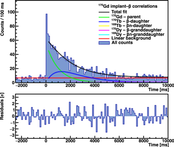
Figure 2. Fit to implant-β-particle detection time correlation histograms for the decay of 170Gd. The black line represents the total fit function, and the red line shows the uncorrelated background. The green, blue, and purple lines indicate the contributions of the parent, the daughter, and the granddaughter activity, respectively.
Download figure:
Standard image High-resolution imageThe number of the neutron-gated β-decay events was derived by fitting an exponential function of the background-subtracted time distribution of implant-β-neutron (i-β-n) correlations. When the statistics was low (below 50 neutrons), numerical integration was used to derive the number of β-delayed neutrons.
The studied isotopes can be divided into three groups based on how the P1n value was determined. The Qβ n values of the lighter REP isotopes are typical below a few hundred keV (e.g., Qβ n = 612 ± 11 keV for 159Pm), or this decay channel might be even closed (Qβ n < 0 keV, e.g., for 161,162Sm or 167−169Gd). The number of the neutron-gated β-decay events for these isotopes was derived by numerical integration and was always found to be consistent with zero. Accordingly, only upper limits for the β-delayed neutron-emission probabilities could be derived.
The number of the neutron-gated β-decay events in the case of several heavier isotopes (e.g.: 161−163Pm and 166−167Eu) was derived not only by numerical integration but also by fitting an exponential function of the background-subtracted time distribution of implant-β-neutron (i-β-n). Always consistent results, with differences well below the statistical uncertainties, were obtained. Figure 3 shows the time distribution of the measured i-β-n correlations after implanting 162Pm isotopes into AIDA. The lines correspond to the fit function (black) including the exponential component (green) and a fixed background (red) extracted from a linear fit to the backward-time distribution of i-β-n correlations.
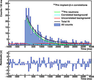
Figure 3. Fit to implant-β-1n time correlation histograms for the decay of 162Pm. The black line represents the total fit function, the red and blue lines show the correlated and uncorrelated background, respectively, and the green line indicates the parent decay.
Download figure:
Standard image High-resolution imageOnly a few hundred (or even fewer) ions of the most neutron-rich isotopes (166Pm, 167,168Sm, 170Eu, and 170−172Gd) were implanted in the AIDA detector. Accordingly, the number of the measured i-β-n correlations were typically very low (e.g., fewer than 15 events in the decay chains of 165,166Pm nuclei), and the statistical errors exceed 30%. Furthermore, in these cases, the daughter isotope is typically a delayed neutron emitter with moderate emission probability. For these exotic isotopes, as a conservative estimate, only upper limits—calculated with a 95% confidence level—for the P1n values were derived assuming that all measured neutrons belong to the decay of the parent nucleus.
Figure 4 shows the measured half-lives compared to recent literature data (Wu et al. 2017) and to theoretical predictions of the FRDM2012+QRPA+HF, RHB+QRPA, and pnFAM models, respectively (Marketin et al. 2016; Möller et al. 2019; Ney et al. 2020). Furthermore, Figure 5 shows the derived neutron-emission probabilities compared with theoretical predictions calculated using the FRDM2012+QRPA+HF, RHB+QRPA, and pn-RQRPA+HF models (Marketin et al. 2016; Möller et al. 2019; Minato et al. 2021). Table 1 lists the resulting T1/2 and P1n values of all isotopes studied in the present work.
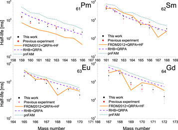
Figure 4. Experimental half-lives derived in the present work (black squares) and taken from the literature (Wu et al. 2017; red circles). Lines show the theoretical values from three models (Marketin et al. 2016; Möller et al. 2019; Ney et al. 2020).
Download figure:
Standard image High-resolution image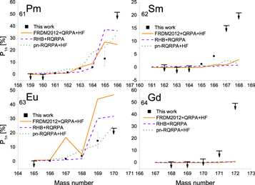
Figure 5. Experimental P1n values derived in this work. Lines show the theoretical values from three models (Marketin et al. 2016; Möller et al. 2019; Minato et al. 2021).
Download figure:
Standard image High-resolution imageTable 1. Half-lives and β-delayed Neutron Emission Probabilities (P1n ) Measured in the Present Work
| Isotope | T1/2 | P1n | Isotope | T1/2 | P1n | Isotope | T1/2 | P1n | Isotope | T1/2 | P1n |
|---|---|---|---|---|---|---|---|---|---|---|---|
| [ms] | [%] | [ms] | [%] | [ms] | [%] | [ms] | [%] | ||||
| 159Pm |

| ≤0.6 | 166Pm |

| ≤52 | 167Sm |

| ≤16 | 170Eu |

| ≤24 |
| 160Pm* |

| ≤0.1 | 161Sm |

| ≤2.7 | 168Sm |

| ≤21 | 167Gd |

| ≤12 |
| 161Pm |

|

| 162Sm |

| ≤1.0 | 165Eu* |

| ≤0.4 | 168Gd |

| ≤0.8 |
| 162Pm |

|

| 163Sm |

| ≤0.1 | 166Eu |

|

| 169Gd* |

| ≤0.7 |
| 163Pm* |

|

| 164Sm |

| ≤0.7 | 167Eu |

|

| 170Gd |

| ≤3 |
| 164Pm |

|

| 165Sm |

|

| 168Eu |

|

| 171Gd |

| ≤10 |
| 165Pm |

|

| 166Sm |

|

| 169Eu |

|

| 172Gd |

| ≤50 |
Note. The half-lives tagged with an asterisk (*) may include both ground-state and isomeric-state decays (for details, see text).
Download table as: ASCIITypeset image
Figure 4 shows that the half-lives agree overall within a factor of three, but it shows some deficiencies for each model. The pnFAM model of Ney (2020) provides longer half-lives in general. The RHB+QRPA from Marketin (2016) almost perfectly reproduces our experimental values for Pm (Z = 61) and Sm (Z = 62), but tends to overpredict the results for Eu (Z = 63) and Gd (Z = 64). The FRDM2012+QRPA+HF model underpredicts the half-lives for the Pm chain, but seems to fit the other three isotopic chains well, apart from a visible kink at N = 105.
The P1n value comparison in Figure 5 shows that for more neutron-rich odd-Z nuclei, the theoretical predictions generally overestimate the P1n values, whereas the trend is inverted for even-Z nuclei in the Sm and Gd chains. Interestingly, the theoretical predictions for Gd (Z = 64) indicate close to zero values in our mass range, while our measurements (although they are all upper limits) show that beyond 171Gd (N = 107), a strong neutron-emission branch is probable. Our data also show that the unusual kink that the FRDM2012+QRPA+HF model predicts for 167,168Eu (N = 104,105) is not reproduced by our data.
This comparison shows the importance of experimental measurements along isotopic chains toward the most neutron-rich nuclei because theoretical models cannot (yet) consistently reproduce the trends. The reason for the discrepancy between the theoretical predictions and the experimental data is most probably the inaccurate knowledge of the Gamow-Teller transition strengths. Accordingly, it is essential to refine theoretical models to increase the precision of the astrophysical simulations.
It should be noted that isomeric states are expected in this mass region (see, e.g., Patel et al. 2017). In order to account for this source of uncertainty, a wide-range variation of fitting variables was executed, including the fitting range of time correlations (starting and end point varied independently), and the energy threshold for β-events. A significant dependence on the starting or the end point of the fitting curve indicates either isomeric states in the decay chain or nuclides with half-lives differing from literature values. Regardless of the source of this discrepancy, the reported half-life values include asymmetric systematic uncertainties calculated from the deviation of the varied fit results. When these effects are suspected, we mark this with asterisks in Table 1. These isotopes are 160,163Pm, 165Eu, and 169Gd.
4. Astrophysical Implication of the Experimental Results
Several authors have proposed that during the r-process freeze-out, the competition between β−-decays and neutron captures shape the REP while the material decays back to stability (Surman et al. 1997; Surman & Engel 2001; Arcones & Martínez-Pinedo 2011; Mumpower et al. 2012). Neutron emission following β−-decays of neutron-rich nuclei may also have a significant impact on the abundance pattern by providing additional neutrons to the environment and changing the mass number of the nuclide. Therefore, it is important to understand the relation between the r-process abundance pattern and nuclear observables, such as β-decay half-lives (T1/2) and β-delayed neutron-emission probabilities (Pn values).
4.1. Method
With respect to the current experimental values and their uncertainties, we perform an uncertainty quantification and a variance-based sensitivity analysis (Saltelli et al. 2010) of the calculated r-process abundance pattern. As discussed in detail below, by treating the physical quantities of interest, namely T1/2 and P1n , as variable inputs of the nuclear reaction network calculation, we can assess their influence on the calculated abundance patterns.
4.1.1. Uncertainty Quantification
Uncertainty quantification reveals how the uncertainties of the nuclear observables collectively translate into the uncertainty of the calculated abundance pattern. This has been performed in various previous studies (Martin et al. 2016; Mumpower et al. 2016; Sprouse et al. 2020), mainly using theoretical values for a wide range of nuclides and focusing on the uncertainty of the overall abundance pattern.
In this work, we perform an uncertainty quantification with the experimental uncertainties of the half-lives and β-delayed one-neutron-emission probabilities (P1n ), specifically focusing on the REP. This assesses the uncertainty of the abundance pattern induced by the current experimental uncertainties. If the size of the induced uncertainty is significantly larger than that of the measured solar abundance, it generally means that a more precise measurement is necessary within the set of nuclides. Because there are other sources of uncertainties from nuclear physics inputs, as well as astrophysical inputs, this uncertainty provides a lower limit.
We further compare these uncertainties of the calculated abundance patterns obtained from this experiment with those calculated with the previously measured β−-decay half-lives taken from Wu et al. (2017), supplemented with the theoretical values from FRDM2012+QRPA (Möller et al. 2019) where previous experimental values do not exist. In this comparison, however, the uncertainties of P1n from the current measurement have been used for both calculations. This is because it is difficult to assume reasonable uncertainties on theoretical values, and as we show in Section 4.2, the largest contribution to the uncertainties comes from the half-lives. Therefore, this comparison quantifies the impact of the current measurements on the β−-decay half-lives.
4.1.2. Variance-based Sensitivity Analysis
In the context of the r-process nucleosynthesis, a notable previous work on sensitivity analysis focusing on nuclear physics inputs in nucleosynthesis calculations has been performed by Mumpower et al. (2016). In their work, sensitivities of the calculated abundances to various nuclear physics observables, such as β-decay half-lives, β-delayed neutron-emission probabilities, neutron capture rates, and masses, were estimated for the entire chart of nuclides.
While this work has provided significant insight into the dependence of the calculated abundances on the individual nuclear physics inputs, their sensitivity analysis method faced several challenges. The sensitivities were estimated by changing one input at a time, with or without propagating the variation to other inputs, and summing the absolute differences of the output from the baseline over all mass numbers. This one-at-a-time scheme implicitly assumes linearity and additivity in the response of the calculation to the change in the input (Saltelli & Annoni 2010). Because nucleosynthesis calculations often show nonlinear relations between variations of reaction/decay rates and abundance changes (Bliss et al. 2020), the sensitivity estimates based on this scheme are potentially unreliable. Furthermore, with this method, the space of the input variables, whose dimension is equal to the number of the variables, is largely unexplored.
Bliss et al. (2020) studied the effect varying the (α, n) reaction rates employing a Monte Carlo approach in the context of neutrino-driven ejecta in core-collapse supernovae. With the Monte Carlo method, it is possible to explore the entire variable space. In identifying the key reaction rates, Spearman's correlation coefficient was employed as sensitivity metric, which assumes a monotonic relation between the output (elemental abundance) and the variation of an input (e.g., an (α, n) reaction rate). While the assumption of a monotonic relation is an improvement from the linear assumption in Rauscher et al. (2016) and Nishimura et al. (2017), who employed Pearson's correlation coefficient, there is no guarantee that the relation is always monotonic.
In our sensitivity analysis, we employ the variance-based sensitivity analysis method. This method is also based on a Monte Carlo approach, and it determines the individual contribution of input variables to the uncertainty (variance) of the output of the model (Saltelli et al. 2010). The same method has recently been applied in a study of ab initio nuclear theory (Ekström & Hagen 2019).
The aim of this work is to apply the sensitivity analysis method to the calculation of r-process abundances in the REP region, with the nuclear reaction network calculation being our model, T1/2 and P1n values from the current experiment being the inputs to be varied, and the abundances as a function of mass number in the REP region being the output of the model. In this study, we compute the first-order sensitivity indices S(1) (see Appendix A), which account for the contributions of the uncertainty of individual variables to the uncertainty (variance) of the output. Because the sensitivity metric is based on the variance, i.e., the size of variation in the output in response to the variation of inputs, it does not rely on any assumption of the type of relation, e.g., monotonic or linear. This allows for a straightforward interpretation of the sensitivity metric and identification of key nuclides and their nuclear properties that are responsible for the uncertainty of the calculated abundance pattern.
Furthermore, this framework allows taking the dependence of the output on multiple input variables (second- or higher-order sensitivity indices) into account, if they exist, which has not been addressed in the previously applied sensitivity analysis methods.
4.1.3. Generation of Monte Carlo Samples
The values of the first-order sensitivity indices S(1) are estimated from the samples generated from Sobol quasi-random sequences. Sobol sequences are deterministic and designed to fill variable spaces more evenly and efficiently than ordinary pseudo-random sequences, which allow a faster convergence of Monte Carlo estimators (Equation (A7)).
In both of the tasks of uncertainty quantification and sensitivity analysis, we use normal (Gaussian) distributions as distributions of most of the experimental values, where the mean values are equal to the nominal experimental values and the standard deviations are equal to the experimental uncertainties. In case of asymmetric uncertainties, the higher values have been used. Picking larger uncertainties to symmetrize the Gaussian distributions greatly simplifies the analysis while providing a conservative estimate of the uncertainty of the abundance pattern. When only upper limits are provided for P1n values, it is assumed that they follow uniform distributions between 0% and the upper limit values (accordingly, if we had lower limits, the distribution would extend from the lower limit value up to 100%).
For the uncertainties of the FRDM2012+QRPA half-lives used in the comparison described in Section 4.1, the size is assumed to be a factor of 10 around the predicted decay rates, following the uncertainty analysis in Mumpower et al. (2016). Any nonphysical samples, such as negative half-lives or P1n values, are discarded.
One thousand samples of each of T1/2 and P1n value have been generated and used as inputs for nuclear reaction network calculations to obtain the nucleosynthesis yields of the r-process. The nuclear reaction network code PRISM (Mumpower et al. 2018) has been used for the calculations. We employ two astrophysical trajectories (temperature and density evolution): a dynamical ejecta from a neutron-star merger, and a neutrino-driven wind. Both scenarios have been extensively studied as some of the most promising sites of the r-process.
The neutron-star merger trajectory is from Vassh et al. (2019) based on the simulations by Rosswog et al. (2013) and Piran et al. (2013), which takes the self-heating based on the FRDM2012 mass model into account (Möller et al. 2016). The hot neutrino-driven wind trajectory (hereafter referred to as hot wind) corresponds to a hot r-process condition with low entropy of S = 30 kB , an initial electron fraction of Ye = 0.20, and an expansion timescale of 70 ms based on Meyer (2002), which is discussed in more detail in Mumpower et al. (2016). In the calculations, it is assumed that the emitted neutrons following the β-decays instantly thermalize, and reach energies equal to the average energy of the neutrons in the environment, which is determined by the temperature of the astrophysical site.
Rates of β−-decays, β−-delayed neutron-emission probabilities, neutron capture rates, fission rates and yields, etc., included in the network are identical to those in Sprouse et al. (2021). Whenever available, the theoretical rates and reaction Q-values have been replaced by the experimental values reported in AME2016 and Nubase2016 (Wang et al. 2017; Audi et al. 2017). For the nuclides measured in this study (Table 1), the current experimental values replace any of the existing β−-decay rates (T1/2) and β-delayed one-neutron-emission probabilities (P1n ).
4.2. Results
Figure 6 shows the ±2σ intervals of the abundances calculated with the samples drawn from the distributions discussed above, allowing variation of the half-lives and P1n values of 159–166Pm, 161–168Sm, 165–170Eu, and 167–172Gd for both of the employed astrophysical trajectories. Derived isotopic solar r-process abundances (Goriely 1999; Sneden et al. 2008) are also shown for reference. The averages of the abundance patterns have been scaled at A = 157 to match the calculation of the neutron-star merger scenario. It is common practice to scale either calculated or solar abundance patterns to make a comparison, as they are both relative abundances. In this work, we choose to scale all the abundances to match A = 157, which is the base of the REP on the low-mass side. This allows for a clear comparison of the height of the peaks of the calculated and the solar abundance patterns. While the calculations do not provide a great match to the solar abundances, the idea of this work is to learn about the dependence of calculated abundances in the REP region on the varied nuclear physics inputs, using some of the representative astrophysical conditions. In order to identify the cause of the significant discrepancies between the calculated abundance patterns and the solar abundance pattern, it is necessary to quantify the abundance uncertainties due to the assumptions and approximations in the astrophysical trajectories, in addition to the quantification of nuclear physics uncertainties.
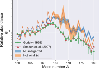
Figure 6. Calculated relative r-process abundance pattern for the neutron-star merger scenario (blue line) and the hot wind scenario (orange). The band represents the ±2σ interval propagated from the uncertainties of the current experimental results. The green boxes and red triangles indicate the derived relative solar r-process abundance pattern from Goriely (1999) and Sneden et al. (2008). The abundance patterns are scaled to match the mean value of the calculated abundance in the neutron-star merger scenario at A = 157.
Download figure:
Standard image High-resolution imageComparisons between the ±2σ uncertainty bands calculated from the current experimental uncertainties (solid bands) and the uncertainty bands calculated with the previous experimental half-lives taken from Wu et al. (2017), supplemented with the theoretical half-lives from FRDM2012+QRPA (Möller et al. 2019; hatched band), are shown in Figure 7. As stated above, the uncertainty of the theoretical values is assumed to be a factor of 10, following the analysis by Mumpower et al. (2016). Both calculations use the current experimental uncertainties of the P1n values for the β-delayed neutron-emission probabilities. Therefore, this comparison quantifies the impact of the current experimental half-lives.

Figure 7. Comparisons of ±2σ uncertainty bands of the calculated abundance patterns between the current experimental uncertainties of T1/2 and P1n values (solid bands) and the uncertainties of T1/2 from Wu et al. (2017), supplemented with the theoretical half-lives from FRDM2012+QRPA (Möller et al. 2019), where previous experimental values do not exist, with the uncertainties of P1n values also from the current experiment (hatched bands). The top panel corresponds to the neutron-star merger scenario, and the bottom panel corresponds to the hot wind scenario. In both cases, all the abundance patterns are scaled to match the mean of the abundance in the neutron-star merger scenario at A = 157. See text for details.
Download figure:
Standard image High-resolution imageIn the neutron-star merger scenario (Figure 7, top panel), the current experiment reduces the uncertainties for the mass numbers A = 162–176. The reduction is especially significant for A = 162–166 and 169–172. For the hot wind scenario (Figure 7, bottom panel), while the reduction in uncertainty is not as significant, the effect of the new data can be seen at A = 165–167 and A = 169–170.
In both trajectories, Figures 6 and 7 show that the current experimental data still have significant effect on the uncertainties of the right (heavier) wing of the REP. Therefore, in our analysis below, we mainly focus on the abundances of the mass numbers A = 168–173 and identify the sources of the uncertainty within the current set of experimental values. Because this analysis accounts only for the uncertainty of the current measurements, it should be noted that the size of uncertainty on the abundance pattern represents only a lower limit.
Figure 8 shows a snapshot of the r-process path (at t = 0.608 s) of the neutron-star merger scenario. The location of the isotopes of interest in the chart of nuclides relative to the path suggests that they are completely synthesized during freeze-out when the material decays back to stability. Therefore, analyzing how the decay properties such as half-lives and P1n affect the abundances around the REP through the variance-based sensitivity analysis may provide further insights into the freeze-out of the r-process. Because most of the analyses below will be common for both trajectories, i.e., neutron-star merger and hot wind, we primarily focus on the neutron-star merger scenario.

Figure 8. A snapshot of the r-process path in the neutron-star merger scenario at t = 0.608 s. The purple squares show the isotopes whose half-lives and β-delayed neutron-emission probabilities have been measured in this work. The solid gray boxes indicate the isotopes with negative one-neutron separation energies (S1n < 0) in the FRDM2012 mass model (Möller et al. 2016). The inset shows the temperature and density profile of the trajectory.
Download figure:
Standard image High-resolution image4.2.1. First-order Sensitivity Indices
First-order sensitivity indices S(1) estimate the amount of the contribution of each variable (T1/2 and P1n values, in this study) to the variance of the abundances. Tables 2 and 3 show the nuclides with the highest S(1) values, which means the largest contribution to the abundance variances, for A = 168–173, for the neutron-star merger and hot wind trajectory, respectively. A more detailed introduction to the variance-based sensitivity analysis method is provided in Appendix A, and complete tables of the sensitivity indices can be found in Appendix B.
Table 2. Table of Nuclear Input Variables that Have a Significant Contribution to the Uncertainties of the Calculated Abundances for A = 168–173 in the Neutron-star Merger Scenario
| Max. relative | 100  (95% C.I.) [%] (95% C.I.) [%] | |||||||
|---|---|---|---|---|---|---|---|---|
| Nuclide | Variable | uncertainty [%] | A = 168 | 169 | 170 | 171 | 172 | 173 |
| 165Pm | T1/2 | 37.4 | 1.9 (±1.1) | 3.2 (±1.5) | 4.9 (±1.9) | 2.7 (±1.5) | 0.8 (±0.9) | — |
| 166Pm | T1/2 | 57.5 | — | — | 0.5 (±0.6) | 0.7 (±0.7) | — | — |
| 166Sm | T1/2 | 15.9 | — | 1.7 (±1.2) | 4.8 (±1.9) | 3.8 (±1.7) | 1.5 (±1.0) | 0.8 (±0.7) |
| 167Sm | T1/2 | 24.9 | 0.6 (±0.6) | — | — | 1.1 (±0.9) | 0.9 (±0.8) | 0.6 (±0.7) |
| 168Sm | T1/2 | 59.5 | 60.9 (±6.6) | 55.1 (±7.1) | 14.6 (±4.4) | 32.6 (±5.0) | 43.5 (±5.5) | 41.6 (±5.6) |
| 168Eu | T1/2 | 10.9 | 0.5 (±0.7) | — | — | — | — | — |
| 169Eu | T1/2 | 23.7 | — | 3.6 (±1.4) | — | — | 0.9 (±0.8) | 0.7 (±0.7) |
| 170Eu | T1/2 | 37.6 | — | — | 0.6 (±0.9) | — | — | — |
| 167Gd | T1/2 | 80.1 | 6.1 (±2.5) | 26.6 (±4.3) | 34.2 (±6.2) | 14.6 (±3.9) | 3.5 (±1.8) | 1.2 (±1.1) |
| 168Gd | T1/2 | 15.8 | 24.3 (±4.6) | 8.3 (±2.7) | 8.1 (±2.8) | 2.2 (±1.5) | — | — |
| 169Gd | T1/2 | 11.0 | — | 0.8 (±0.8) | — | — | — | — |
| 170Gd | T1/2 | 13.9 | — | — | 25.2 (±4.7) | 1.4 (±1.2) | 2.6 (±1.4) | 3.5 (±1.7) |
| 171Gd | T1/2 | 37.0 | — | — | — | 20.5 (±4.1) | 4.6 (±2.0) | 1.0 (±1.1) |
| 172Gd | T1/2 | 69.3 | — | — | — | 3.6 (±2.1) | 35.7 (±5.1) | 49.3 (±5.9) |
| 165Pm | P1n | 47.0 | — | 0.6 (±0.6) | 0.7 (±0.5) | — | — | — |
| 168Sm | P1n | (100) | — | — | — | 0.8 (±0.8) | 0.6 (±0.6) | — |
| 169Eu | P1n | 39.8 | 5.4 (±2.1) | — | 3.7 (±1.6) | 3.6 (±1.7) | 1.3 (±1.0) | 0.6 (±0.7) |
| 170Eu | P1n | (100) | — | 0.5 (±0.6) | — | — | — | — |
| 172Gd | P1n | (100) | — | — | — | 5.5 (±2.0) | 3.2 (±1.5) | 0.6 (±0.7) |
 total: total: | 94.9 (±8.6) | 100.1 (±9.2) | 93.9 (±9.9) | 84.0 (±8.5) | 95.1 (±8.3) | 99.7 (±8.6) | ||
 total: total: | 5.9 (±2.3) | 1.1 (±1.1) | 5.6 (±2.0) | 11.0 (±2.9) | 5.7 (±2.0) | 2.0 (±1.1) | ||
| S(1) total: | 100.9 (±8.9) | 101.3 (±9.2) | 99.5 (±10.1) | 95.0 (±9.0) | 100.7 (±8.6) | 101.6 (±8.6) | ||
Note. Columns 4–9 show the first-order sensitivity indices (S(1)), which represent the contribution of individual variables to the abundance uncertainty, with 95% confidence intervals. The maximum relative uncertainty (third column) is the ratio of the size of the larger one of the upper or lower experimental uncertainties to the nominal value, in percent. (100) indicates that the P1n
value only has an upper limit and the size of its relative uncertainty is 100%, according to the convention in Dimitriou et al. (2021). Long dashes (—) indicate that the nominal value of  is lower than 0.5 [%]. Values higher than 10 [%] are highlighted in boldface. Complete tables are given in Appendix B.
Download table as: ASCIITypeset image
From Tables 2 and 3, it can be seen that samarium (Z = 62) and gadolinium isotopes (Z = 64) account for most of the abundance variances for these mass numbers for both astrophysical scenarios. For example, in the case of the neutron-star merger scenario, based on the values of the sensitivity indices, it can be concluded that the half-lives of 168Sm and 168Gd account for 60.9 (±6.6)% and 24.3 (±4.6)% of the variance (propagated uncertainty) of the abundances at A = 168, respectively. The effect of the half-life of 168Sm also propagates to the uncertainties of abundances for A = 172 and 173, which is discussed in more detail below. On the other hand, the influence of the P1n values is relatively small in this astrophysical scenario.
Table 3. Table of Nuclear Physics Inputs that Have a Significant Contribution to the Uncertainties of Calculated Abundances for A = 168–173 in the Hot Wind Scenario
| Max. Relative | 100  (95% C.I.) [%] (95% C.I.) [%] | |||||||
|---|---|---|---|---|---|---|---|---|
| Nuclide | Variable | uncertainty [%] | A = 168 | 169 | 170 | 171 | 172 | 173 |
| 165Pm | T1/2 | 37.4 | — | 0.5 (±0.6) | — | — | — | — |
| 168Sm | T1/2 | 59.5 | 96.1 (±14.1) | 71.4 (±7.0) | 95.2 (±8.2) | 56.8 (±7.1) | 44.6 (±7.2) | 80.7 (±13.3) |
| 169Eu | T1/2 | 23.7 | — | 2.6 (±1.4) | 0.5 (±0.6) | — | — | — |
| 167Gd | T1/2 | 80.1 | — | 0.6 (±0.6) | — | — | — | — |
| 168Gd | T1/2 | 15.8 | — | 2.8 (±1.5) | — | — | — | — |
| 170Gd | T1/2 | 13.9 | — | — | 1.1 (±0.9) | 0.7 (±0.8) | — | — |
| 171Gd | T1/2 | 37.0 | — | — | — | 6.9 (±2.6) | 0.5 (±0.7) | 1.8 (±1.2) |
| 172Gd | T1/2 | 69.3 | — | — | — | 9.9 (±3.2) | 53.3 (±7.6) | 11.1 (±3.3) |
| 168Sm | P1n | (100) | 2.0 (±1.5) | 3.5 (±1.7) | 0.5 (±0.6) | — | — | — |
| 169Eu | P1n | 39.8 | 1.0 (±0.9) | 10.8 (±2.9) | 0.5 (±0.7) | — | — | — |
| 170Eu | P1n | (100) | — | 6.7 (±2.3) | 2.1 (±1.2) | — | — | — |
| 172Gd | P1n | (100) | — | — | — | 25.2 (±4.6) | 2.6 (±1.7) | 5.5 (±2.1) |
 total: total: | 97.0 (±14.1) | 78.9 (±7.4) | 97.4 (±8.3) | 74.6 (±8.2) | 98.6 (±10.5) | 93.8 (±13.7) | ||
 total: total: | 3.0 (±1.8) | 21.5 (±4.1) | 3.7 (±1.6) | 25.9 (±4.7) | 2.8 (±1.7) | 5.6 (±2.1) | ||
| S(1) total: | 100.0 (±14.3) | 100.5 (±8.5) | 101.1 (±8.4) | 100.5 (±9.5) | 101.3 (±10.7) | 99.4 (±13.9) | ||
Note. Columns 4–9 show the first-order sensitivity indices (S(1)), which represent the contribution of individual variables to the abundance uncertainty, with 95% confidence intervals. The maximum relative uncertainty (third column) is the ratio of the size of the larger one of the upper or lower experimental uncertainties to the nominal value, in percent. (100) indicates that the P1n
value only has an upper limit and the size of its relative uncertainty is 100%, according to the convention in Dimitriou et al. (2021). Long dashes (—) indicate that the nominal value of  is lower than 0.5 [%]. Values higher than 10 [%] are highlighted in boldface. Complete tables are given in Appendix B.
Download table as: ASCIITypeset image
In the case of the hot wind scenario, a larger contribution from the uncertainty of the P1n values has been observed on average (Table 3). This is likely because the environment is less neutron-rich than in the neutron-star merger scenario (Mumpower et al. 2016). Therefore, β-delayed neutron emissions become a more important source of neutrons, especially at the late time of the r-process.
As a general trend, the uncertainties of the half-lives have the largest effect on the abundances for the corresponding mass number of the isotope, and a smaller effect for higher mass numbers. As one might expect, one-neutron-emission probabilities (P1n ) can influence the abundance for the mass number A − 1, where A is the mass number of the parent nucleus. For example, the uncertainty of P1n (165Pm) accounts for 59.7% of the variance for A = 164 in the neutron-star merger scenario.
4.2.2. Effect of the Size of the Uncertainty
Maximum relative uncertainties of each input variable, which we define to be the size of the ratio of the larger one of upper or lower uncertainty to the nominal value, are also shown in the third column of Tables 2 and 3. The half-lives of 168Sm, 167Gd, and 172Gd, which are some of the most influential half-lives in the neutron-star merger scenario within the current data set, all have relatively large uncertainties of 60%–80%. However, a large relative uncertainty does not necessarily mean a large influence on the abundance uncertainty, as can be seen from Tables 2 and 3. For example, the half-life of 172Gd, whose relative uncertainty is larger than that of 168Sm, has a similar or smaller contribution to the abundance at A = 172 and 173 than 168Sm, which may also suggest that the mechanisms of the abundance pattern formation are different between inside the REP (A = 155–170) and the heavy-mass wing of the peak (A > 170).
In order to investigate the effect of the size of input uncertainty on the sensitivity indices, we conduct a test under the neutron-star merger condition. In this test, the size of the uncertainty of the half-life of 168Sm, which has been identified as one of the most influential inputs in both of the astrophysical trajectories, is artificially decreased to the relative uncertainty of 20% from the current value of 59.5%, while the mean value is kept the same. Note that this does not consider the possibility that the true mean value of the half-life can lie outside the currently considered 20% relative uncertainty.
In the neutron-star merger scenario, the half-life of 168Sm has first-order sensitivity indices of S(1) = 60.9%, 43.5%, and 41.6% for A = 168, 172, and 173, respectively (Table 2) when the the relative uncertainty is 59.5%. This means that if the half-life could be fixed without any uncertainty, we would be able to reduce the uncertainty of the calculated abundances by 60.9%, 43.5%, and 41.6% for A = 168, 172, and 173, respectively. Because experimentally fixing the half-life or any other observables without uncertainty is impossible, it is worthwhile to investigate the effect of reducing the uncertainty.
Figure 9 shows a comparison between the calculated uncertainty (variance) of the abundance pattern using the original experimental uncertainty (light blue) and when the relative uncertainty of the half-life of 168Sm is reduced to 20% from 59.5% (dark blue) in the neutron-star merger scenario. As predicted from the sensitivity indices (see Tables 2 and B2), the uncertainties have been significantly reduced for A = 168 and 169, and to a smaller degree for the higher mass numbers.
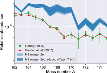
Figure 9. Calculated relative r-process abundance pattern for the neutron-star merger scenario (blue line). The green boxes and red triangles are the derived relative solar r-process abundance pattern from Goriely (1999) and Sneden et al. (2008). The band in light blue represents the ±2σ interval propagated from the uncertainties of the original experimental results. The band in dark blue represents the ±2σ interval when the relative uncertainty of the half-life of 168Sm is artificially reduced to 20%, with the same mean value. All the abundance patterns are scaled to match the mean of the calculated abundances at A = 157 for the neutron-star merger scenario.
Download figure:
Standard image High-resolution imageTable 4 shows the sensitivity indices with the reduced 168Sm half-life uncertainty. While the value of  of the half-life of 168Sm for A = 168 decreased to 17.6% from 60.9% (Table 2), it is still a significant contribution to the output variances. It is also worth pointing out that the half-life of 168Gd now has a larger contribution to the variance at A = 168, although its relative uncertainty is only 15.8%. For the mass numbers A = 172 and 173, now the half-life of 172Gd has the dominant contributions. At the same time, it can be seen from the table that the sensitivity has been more fragmented across the input variables compared to the case shown in Table 2, elevating the relative sensitivity of the half-lives of the gadolinium isotopes.
Table 4. Table of Nuclear Input Variables that Have a Significant Contribution to the Uncertainties of the Calculated Abundances for A = 168–173 for the Neutron Star Merger Scenario, with the Relative Uncertainty of the Half-life of 168Sm Reduced to 20.0%
| Max. relative | 100  (95% C.I.) [%] (95% C.I.) [%] | |||||||
|---|---|---|---|---|---|---|---|---|
| Nuclide | Variable | uncertainty [%] | A = 168 | 169 | 170 | 171 | 172 | 173 |
| 165Pm | T1/2 | 37.4 | 3.5 (±1.5) | 5.9 (±2.0) | 5.4 (±2.2) | 3.6 (±1.8) | 1.3 (±1.1) | 0.6 (±0.7) |
| 166Pm | T1/2 | 57.5 | — | 0.6 (±0.4) | 0.5 (±0.6) | 0.8 (±0.7) | 0.5 (±0.6) | — |
| 166Sm | T1/2 | 15.9 | 0.8 (±0.7) | 3.1 (±1.6) | 5.2 (±2.0) | 4.9 (±2.0) | 2.2 (±1.2) | 1.1 (±0.9) |
| 167Sm | T1/2 | 24.9 | 1.4 (±1.0) | 0.5 (±0.6) | — | 1.5 (±1.1) | 1.5 (±1.1) | 1.0 (±0.9) |
| 168Sm | T1/2 | 20.0* | 17.6 (±3.8) | 13.0 (±3.3) | 1.0 (±0.9) | 9.4 (±2.8) | 12.1 (±3.1) | 9.7 (±2.8) |
| 167Eu | T1/2 | 8.9 | — | 0.5 (±0.6) | — | — | — | — |
| 169Eu | T1/2 | 23.7 | — | 7.1 (±2.1) | — | 0.6 (±0.7) | 1.4 (±1.1) | 1.0 (±0.9) |
| 170Eu | T1/2 | 37.6 | — | — | 0.8 (±0.9) | — | — | — |
| 167Gd | T1/2 | 80.1 | 12.5 (±4.3) | 50.8 (±6.4) | 39.7 (±6.8) | 19.8 (±4.9) | 5.4 (±2.4) | 1.8 (±1.4) |
| 168Gd | T1/2 | 15.8 | 50.6 (±6.9) | 16.0 (±3.5) | 9.5 (±2.9) | 3.0 (±1.7) | 0.6 (±0.8) | — |
| 169Gd | T1/2 | 11.0 | — | 1.6 (±1.1) | — | — | — | — |
| 170Gd | T1/2 | 13.9 | — | — | 29.2 (±5.2) | 1.9 (±1.4) | 4.1 (±1.8) | 5.5 (±2.1) |
| 171Gd | T1/2 | 37.0 | — | — | — | 28.0 (±4.8) | 7.0 (±2.7) | 1.5 (±1.5) |
| 172Gd | T1/2 | 69.3 | — | — | — | 4.8 (±2.5) | 54.4 (±6.1) | 73.8 (±6.9) |
| 165Pm | P1n | 47.0 | — | 1.2 (±0.8) | 0.9 (±0.5) | 0.6 (±0.4) | — | — |
| 168Sm | P1n | (100) | — | — | 0.6 (±0.8) | 1.4 (±1.0) | 1.1 (±0.7) | 0.7 (±0.6) |
| 169Eu | P1n | 39.8 | 11.3 (±3.0) | — | 4.5 (±1.8) | 5.0 (±2.1) | 2.1 (±1.3) | 1.0 (±0.8) |
| 172Gd | P1n | (100) | — | — | — | 7.4 (±2.4) | 4.8 (±1.8) | 0.9 (±0.8) |
Note. Columns 4–8 show the first-order sensitivity indices (S(1)), which represent the contribution of individual variables to the abundance uncertainty, with 95% confidence intervals. The maximum relative uncertainty (third column) is the ratio of the size of the larger one of the upper or lower experimental uncertainties to the nominal value, in percent. (100) indicates that the P1n
value only has an upper limit and the size of its relative uncertainty is 100%, according to the convention in Dimitriou et al. (2021). 20.0* for the half-life of 168Sm denotes that the relative uncertainty is artificially reduced to 20.0%. Long dashes (—) indicate that the nominal value of  is lower than 0.5 [%].
Download table as: ASCIITypeset image
Therefore, the half-lives of gadolinium isotopes may be considered significant sources of uncertainty of the calculated abundances in addition to the 168Sm half-life within the set of isotopes of interest in the current study.
4.2.3. Impact of 168Sm Half-life During the Freeze-out
By inspecting the samples generated for the variance-based sensitivity analysis, one may learn how the abundances depend on the nuclear physics inputs. We again take the half-life of 168Sm as an example to demonstrate this, focusing on the neutron-star merger scenario. Figure 10 shows the correlations of abundances for several mass numbers with the half-life of 168Sm. Comparing panels (a) and (b) of the figure, it can be seen that the abundance has a clear correlation with the half-life when the sensitivity index is high.
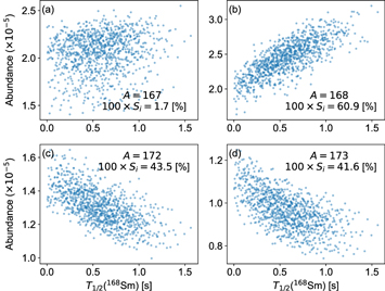
Figure 10. Correlation of abundances for A = 167, 168, 172, and 173 with the half-life of 168Sm, as well as the first-order sensitivity indices (S(1)), in the neutron-star merger scenario. The correlation is sharp for a high sensitivity index (e.g., panel (b)), and the distribution is blurred for a low sensitivity index (e.g., panel (a)).
Download figure:
Standard image High-resolution imageThe mechanism of this correlation becomes clear by analyzing the abundance flows due to β-decay and neutron capture. Figure 11 shows the relative isotopic abundances as functions of time (upper panels), the abundance flows (middle panels), and their total contributions, i.e., integrals of the abundance flows over time (lower panels) due to neutron capture and β-decay (labeled (n, γ) and β− in the figure, respectively) for 168Sm, 168Eu, and 168Gd. They are separated into two cases: the sampled half-life of 168Sm is longer than 0.55 [s] (Case 1) or shorter than 0.20 [s] (Case 2) for the neutron-star merger scenario. The dashed red lines in the upper and middle panels represent the relative abundance of neutrons as a function of time.

Figure 11. The top panels (a)–(c) show the abundance evolution of the isotopes 168Sm, 168Eu, and 168Gd as functions of time in the neutron-star merger scenario. The vertically hatched yellow bands correspond to the case where the half-life of 168Sm exceeds 0.55 [s], and the solid gray bands correspond to a half-life shorter than 0.20 [s]. The middle panels (d)–(f) show the abundance flows of β−-decay (labeled β−, hatched with "//") and neutron capture (labeled (n, γ), solid bands) as functions of time, for 168Sm, 168Eu, and 168Gd, respectively, extracted from the generated samples. The dash–dotted red line is the neutron abundance as a function of time, which shows that these isotopes are synthesized after the neutron abundance significantly drops (freeze-out). The bottom panels (g)–(i) show the integrals of the abundance flows, i.e., the areas below the solid and dotted lines in the top panels. In all the panels, the solid outlines represent Case 1: T1/2(168Sm) > 0.55 [s], and the dashed outlines represent Case 2: T1/2(168Sm) < 0.20 [s].
Download figure:
Standard image High-resolution imageIt shows that these isotopes are synthesized after the neutron abundance drops significantly (freeze-out). The total contributions of the flows of (n, γ) and β− are also shown in Figure 12 for the isotopic chains of Sm, Eu, and Gd up to the mass number A = 172. In the figure, the width of the arrows correspond to the total amount of (n, γ) and β−-decay flows. Contributions from the reverse reaction of neutron capture (i.e., photodissociation) are negligible for all cases. Flows due to β-delayed neutron emission are also not shown because they only have contributions up to a few percent on average in this neutron-star merger scenario (Table 2).

Figure 12. The arrows show the total abundance flow (same quantity as in panels (g)–(i) in Figure 11), averaged over the generated samples in the neutron-star merger scenario. Red corresponds to the case where the half-life of 168Sm is shorter than 0.20 [s], and blue shows a half-live longer than 0.55 [s]. Panels (b) and (c) focus on the flows from 172Gd and 168Gd, respectively. The propagated influence of the half-life of 168Sm is visible, which results in affecting the final abundances.
Download figure:
Standard image High-resolution image
Panel (d) of Figure 11 shows that the half-life of 168Sm has a significant effect on the abundance flow from the isotope due to β-decay, while leaving the flow due to neutron capture relatively unaffected. The integrated abundance flow from 168Sm shown in panel (g) indicates that the flow due to β-decay is increased when the half-life of 168Sm is small. The increased amount of 168Eu is quickly consumed by neutron captures, as shown in pink in panels (e) and (h). This in turn means that the longer half-life of 168Sm provides a smaller amount of 168Eu that can be converted into higher masses through neutron capture, therefore resulting in the smaller abundances for higher mass numbers, as shown in panels (c) and (d) of Figure 10. This effect can also be seen in panels (a) and (b) of Figure 12 and explains why the abundances for A = 172 or 173 decrease as the half-life of 168Sm increases.
This means that the half-life of 168Sm has a significant influence on the neutron capture flow in the Eu isotopic chain because 168Sm is synthesized almost at the same time as the neutron abundance starts to drop (panel (a), Figure 11), meaning that some neutrons are still available for neutron capture, while photodissociation is no longer active. In panel (i) of Figure 11 and panel (b) of Figure 12, it can be seen that the flow from 168Gd due to β-decay (hatched histogram in blue) is larger when the half-life of 168Sm is longer. This is because the longer half-life of 168Sm extends the flow of β-decay of 168Eu into the late time of the r-process where neutron capture is no longer significantly active, thus leaving more material at the same isobaric mass chain by avoiding being consumed by neutron capture.
Overall, the half-life of 168Sm affects not only the flow of β-decay of 168Sm, but also the flow of neutron capture in the Eu isotopic chain up to a mass number A = 172, 173 and higher. This is also the case in the Gd isotopic chain, but to a lesser extent. The balance between the β-decays and the neutron captures determines the final abundance pattern. Therefore, in order to properly account for the uncertainties of the abundance pattern from the nuclear physics inputs, uncertainties of neutron capture rates have to be included as well. This will be addressed in future work.
5. Summary and Conclusions
The β-decay properties of 28 neutron-rich Pm, Sm, Eu, and Gd isotopes were measured at RIKEN Nishina Center. Using the BRIKEN neutron counter array, β-delayed neutron-emission probabilities were derived for the first time in this mass region. The existing half-life database has been significantly extended toward more neutron-rich species.
Nuclear reaction network calculations for the r-process employing a neutron-star merger and a hot wind scenario have been carried out. Uncertainty quantification through the network calculations and comparison with the previous measurement supplemented with the assumed theoretical uncertainties showed that the currently measured half-lives reduce the propagated uncertainty (variance) of the calculated abundances of the heavier wing of the REP.
A new variance-based sensitivity analysis method has been introduced to identify nuclear physics inputs of importance within the current experimental uncertainties. The analysis has been performed using the characteristic abundance pattern of the REP region.
The results of the analysis indicate that only a handful of variables account for nearly all the uncertainty (variance) of the abundance pattern. The results also suggest that the contributions of the uncertainty of the currently measured β-delayed one-neutron-emission probabilities (P1n ) are significantly smaller than the half-lives in the case of neutron-star mergers. The uncertainties of the P1n values have larger contributions to the abundance pattern in the hot wind scenario, most likely because the environment is poorer in neutrons than in the neutron-star merger scenario.
The half-life of 168Sm, which has been measured for the first time in the current experiment, shows a significant influence on the high-mass tail of the REP (A = 168–173) in both astrophysical scenarios. The calculated sensitivity indices and the numerical experiment on artificially reducing the uncertainty of the half-life of 168Sm also indicate that the half-lives of 167–172Gd are significant sources of the uncertainty on the calculated abundance patterns. The analysis of the abundance flows due to neutron captures and β-decays in the neutron-star merger scenario revealed that when the timescales of the β-decays of 168Sm and neutron captures are comparable, the material can be transferred to higher masses such as A = 172 and 173 through chains of neutron capture mainly within the Eu isotopic chain.
The high sensitivity of the abundances to the half-life of 168Sm is most likely due to 168Sm being synthesized at the beginning of the r-process freeze-out when some neutrons are still available for neutron capture. This sensitivity analysis method thus provides a detailed view of how the flows of material in the r-process are affected by the nuclear physics inputs, in addition to identifying influential input variables.
In general, the observation that only a handful of nuclides contribute to the uncertainty of the abundance pattern is consistent with the fact that the r-process nuclear reaction network is a highly overparameterized model. This means that the number of input variables (rates, initial condition, astrophysical trajectory, etc.) is larger than the number of output variables (abundances).
From a large number of input variables, the variance-based sensitivity analysis method can effectively identify influential variables, as demonstrated above, by focusing on localized features of the abundance pattern and a subset of input variables. This method relies on an assumption that the variables of interest have reasonable uncertainties. If experimental uncertainties are not available, which is currently the case for many of the nuclear observables of neutron-rich nuclei, theoretical uncertainties would be required to identify influential input variables.
The astrophysical analysis in this work does not concern theoretical β-decay properties of nuclei that are outside of the current experiment. However, as shown in Figure 4, some systematic discrepancies between the observed β-decay half-lives and the theoretical predictions are present. In future work, it may be useful to calibrate the theoretical predictions based on the available experimental data and perform uncertainty quantification and a sensitivity analysis in order to investigate the implication on the trend of β-decay properties by the experimental data and its effect on calculated abundance patterns. Furthermore, it will be necessary to include more isotopes as well as more nuclear observables, such as masses and neutron capture rates, to draw more general conclusions. The possible dependence between the observables, e.g., masses and β−-decay half-lives, should also be accounted for within the sensitivity analysis method.
This work was supported by the National Research, Development, and Innovation Fund of Hungary, financed under the K18 funding scheme (Project No. NN128072 and K128729). Y.S., I. D., R. C. F. and C. J. G. acknowledge funding from the Canadian Natural Sciences and Engineering Research Council (NSERC): SAPIN-2019-00030; Canadian Natural Sciences and Engineering Research Council (NSERC): SAPPJ-2017-00026. This work was supported by National Science Foundation (NSF) under grant No. PHY-1714153 (AE, NN), by JSPS KAKENHI (grants Nos. 17H06090 and 20H05648) and the RIKEN program for Evolution of Matter in the Universe (r-EMU). P.J.C.S., T.D., O.H., L.J.H.B., D.K., L.B., and P.J.W. acknowledge the support of the UK Science and Technology Facilities Council (STFC). This research was sponsored in part by the Office of Nuclear Physics, U.S. Department of Energy (DOE) under Award No. DE-FG02-96ER40983 (UTK) and DE-AC05-00OR22725 (ORNL), and by the National Nuclear Security Administration (NNSA) under the Stewardship Science Academic Alliances program through DOE Award No. DE-NA0002132. This work was supported by US National Science Foundation award PHY-1714153. This work was supported by the Spanish MICINN grants FPA2014-52823-C2-1-P, FPA2017-83946-C2-1-P (MCIU/AEI/FEDER); Ministerio de Ciencia e Innovacion grant PID2019-104714GB-C21; Centro de Excelencia Severo Ochoa del IFIC SEV-2014-0398 and Generalitat Valenciana PROMETEO/2019/007. A.A. acknowledges partial support of the JSPS Invitational Fellowships for Research in Japan (ID: L1955). M.P.-S. received funding from the Polish National Science Centre under grants Nos. 2019/33/N/ST2/03023 and 2020/36/T/ST2/00547. A.K. was partially funded by grant No. 2020/39/B/ST2/02346. Y.S. would like to thank Nicole Vassh (U of Notre Dame/TRIUMF) for providing the neutron-star merger trajectory and the initial abundance distributions. This research was enabled in part by computing resources provided by WestGrid (www.westgrid.ca) and Compute Canada (www.computecanada.ca). F.M. acknowledges the support of ANID/FONDECYT Regular 1171467 and ANID/FONDECYT Regular 1221364 national projects.
Appendix A: Introduction to the Variance-based Sensitivity Analysis Method
The variance-based sensitivity method applied in this work is based on the work presented in Saltelli et al. (2010), and the notation in this section follows that of the paper. We refer the reader to Saltelli et al. (2010) and Mara et al. (2015) for more detailed discussions of the method. As explained in the main text of the current work, this method quantifies the contribution of the uncertainty (variance) of each input variable to the uncertainty of the output. In our work, the input variables correspond to the experimental β-decay half-lives (T1/2) and the one-neutron-emission probabilities (P1n ), and the output corresponds to the nuclear abundances as a function of mass numbers. A more detailed introduction to the variance-based sensitivity analysis method is provided below.
Suppose that a numerical model can be expressed as Y = f(X1, X2,...,Xk ), where Y is the output (e.g., nuclear abundance for a given mass number), Xi (i = 1, 2,...,k) are the input variables (e.g., T1/2 and P1n values), and f( ·) is the simulation (e.g., nucleosynthesis postprocessing code). Assuming for now that X1, X2,...,Xk are independently and uniformly distributed in [0, 1], the following decomposition of the overall output variance V(Y) is proven unique by Sobol (1993):

where Vi is the output variance due to the variance of input variable Xi , and the definition is similar for Vij and other higher-order terms. Dividing both sides by V(Y),

where  is called a first-order sensitivity index for Xi
,
is called a first-order sensitivity index for Xi
,  is a second-order sensitivity index, and so on. These partial variances
  ,
,  and so on can be written as (see Sobol 1993; Saltelli et al. 2010 for more details)

and so on. In Equation (A3),  denotes the expectation value (average) of Y when the value of Xi
is fixed, and
denotes the expectation value (average) of Y when the value of Xi
is fixed, and  means that the average is taken over all the possible values of all the variables except for Xi
. The outer
means that the average is taken over all the possible values of all the variables except for Xi
. The outer  denotes that variance of the expected value is computed over all the possible values of Xi
. More intuitively, this is equivalent to calculating the average of the samples shown in Figure 10 by slicing the samples at a given value of the half-life and then estimating how much the average varies as the samples are sliced at all the possible values of the half-life. Therefore, the sensitivity indices can be written as
denotes that variance of the expected value is computed over all the possible values of Xi
. More intuitively, this is equivalent to calculating the average of the samples shown in Figure 10 by slicing the samples at a given value of the half-life and then estimating how much the average varies as the samples are sliced at all the possible values of the half-life. Therefore, the sensitivity indices can be written as

and so on, where  .
.
While we have assumed so far that the input variables are uniformly distributed in [0, 1], this method can be used with general distributions such as a normal distribution or uniform distributions that are not in [0, 1], because random numbers uniformly distributed in [0, 1] can be transformed to desired distributions through inverse transform sampling, as long as they are independently distributed and their cumulative distribution functions are known. The sensitivity indices can then be defined in a similar manner for general distributions (Mara et al. 2015).
A.1. Monte Carlo Estimate of Sensitivity Indices
In practice, the sensitivity indices (e.g., Equations (A5) and (A6)) cannot be computed analytically. Therefore, we compute their Monte Carlo estimates instead. In order to illustrate the Monte Carlo method, we use the first-order sensitivity index (Equation (A5)) as an example.
Suppose that we have k variables of interest and wish to use N samples to compute their Monte Carlo sensitivity estimates. The first step is to generate samples that are uniformly distributed in [0, 1]. While random numbers can be used for this purpose, we employ a Sobol quasi-random sequence implemented in a Python library called SALib (Herman & Usher 2017). Sobol quasi-random sequences are designed to generate multidimensional uniform samples in [0, 1] to efficiently explore the entire variable space by filling the gap between previously sampled points (Saltelli et al. 2010). Using the quasi-random sequence, we generate N × 2k samples and split them into two matrices of size N × k.
The next step is to transform the uniformly distributed samples for each variable in the two matrices into desired distributions. In this study, the half-lives are assumed to follow truncated normal (Gaussian) distributions with their means and standard deviations defined by the experimental values and uncertainties. The beta-delayed one-neutron-emission probabilities (P1n values) are either truncated normal distributions or uniform distributions in [0, (upper limit of P1n )]. The samples uniformly distributed in [0, 1] can be transformed into these distributions through inverse transform sampling. For convenience, we call the first of the two transformed N × k matrices A and the second matrix B . Using these matrices, the first-order sensitivity index is estimated by (based on Equation (16) of Saltelli et al. 2010 and Equation (30) of Mara et al. 2015)
where  denotes a Monte Carlo estimate of
  , and f(
A
)j
as well as f(
B
)j
are the output of simulation run with the j-th row (j = 1, 2,...,N) of the matrices
A
and
B
, respectively.
, and f(
A
)j
as well as f(
B
)j
are the output of simulation run with the j-th row (j = 1, 2,...,N) of the matrices
A
and
B
, respectively. ![${{\boldsymbol{B}}}_{{\boldsymbol{A}}}^{[i]}$](https://content.cld.iop.org/journals/0004-637X/936/2/107/revision1/apjac80fcieqn61.gif) is a N × k matrix whose i-th column (i = 1, 2,...,k) comes from the matrix
A
, but all the other columns come from the matrix
B
. Consequently,
is a N × k matrix whose i-th column (i = 1, 2,...,k) comes from the matrix
A
, but all the other columns come from the matrix
B
. Consequently, ![$f{({{\boldsymbol{B}}}_{{\boldsymbol{A}}}^{[i]})}_{j}$](https://content.cld.iop.org/journals/0004-637X/936/2/107/revision1/apjac80fcieqn62.gif) is the output of the simulation run with the j-th row of
is the output of the simulation run with the j-th row of ![${{\boldsymbol{B}}}_{{\boldsymbol{A}}}^{[i]}$](https://content.cld.iop.org/journals/0004-637X/936/2/107/revision1/apjac80fcieqn63.gif) .
.  is the total variance of the output of the simulation, computed with all the generated samples. Errors of the computed sensitivity indices can be estimated using bootstrapping (Archer et al. 1997).
Appendix B: Complete Tables of First-order Sensitivity Indices
Tables B1 and B2 show the complete first-order sensitivity indices for calculated abundances with mass numbers A = 161–166 and A = 167–173, respectively for the neutron star merger scenario, and Tables B3 and B4 for the hot wind scenario.
Table B1. Table of First-order Sensitivity Indices S(1) for Abundances with Mass Numbers A = 161–166 for the Neutron-star Merger Scenario
| Max. Rel. |
 [%] (95% C.I.) [%] (95% C.I.) | |||||||
|---|---|---|---|---|---|---|---|---|
| Nuclide | Variable | Unc. [%] | A = 161 | 162 | 163 | 164 | 165 | 166 |
| 159Pm | T1/2 | 2.6 | 0.2 (±0.4) | — | — | — | — | — |
| 160Pm | T1/2 | 1.8 | 0.6 (±0.8) | 0.1 (±0.3) | — | — | — | — |
| 161Pm | T1/2 | 2.8 | 2.5 (±1.4) | 0.2 (±0.4) | — | — | — | — |
| 162Pm | T1/2 | 8.1 | — | 21.4 (±3.9) | 1.2 (±1.0) | 2.1 (±1.2) | 0.3 (±0.5) | — |
| 163Pm | T1/2 | 11.6 | — | — | 27.9 (±4.7) | — | 0.4 (±0.5) | 0.5 (±0.5) |
| 164Pm | T1/2 | 13.6 | — | — | — | 4.0 (±1.9) | — | 0.4 (±0.6) |
| 165Pm | T1/2 | 37.4 | 0.1 (±0.3) | — | — | 0.7 (±0.7) | 73.3 (±7.6) | 17.3 (±4.2) |
| 166Pm | T1/2 | 57.5 | — | — | — | — | 0.7 (±0.7) | 2.5 (±1.5) |
| 161Sm | T1/2 | 10.1 | 76.1 (±7.9) | 0.9 (±0.9) | 1.9 (±1.2) | 0.2 (±0.4) | — | — |
| 162Sm | T1/2 | 9.0 | — | 71.9 (±7.5) | 19.9 (±3.8) | 2.6 (±1.4) | 0.5 (±0.6) | 0.1 (±0.3) |
| 163Sm | T1/2 | 11.7 | — | — | 46.6 (±6.2) | — | 0.9 (±0.8) | 0.5 (±0.8) |
| 164Sm | T1/2 | 4.1 | — | — | — | 27.1 (±4.4) | 0.6 (±0.6) | 1.6 (±0.9) |
| 165Sm | T1/2 | 9.3 | — | — | — | — | 5.6 (±2.2) | — |
| 166Sm | T1/2 | 15.9 | 0.1 (±0.2) | — | — | — | 0.2 (±0.3) | 50.2 (±6.2) |
| 167Sm | T1/2 | 24.9 | — | — | — | — | — | — |
| 168Sm | T1/2 | 59.5 | 0.7 (±0.7) | 0.1 (±0.3) | 0.2 (±0.2) | — | — | 0.1 (±0.3) |
| 165Eu | T1/2 | 6.4 | — | — | — | — | 1.5 (±1.1) | 0.8 (±0.8) |
| 166Eu | T1/2 | 11.4 | — | — | — | — | — | 2.5 (±1.3) |
| 167Eu | T1/2 | 8.9 | — | — | — | — | — | — |
| 168Eu | T1/2 | 10.9 | — | — | — | — | — | — |
| 169Eu | T1/2 | 23.7 | — | — | — | — | — | — |
| 170Eu | T1/2 | 37.6 | — | — | — | — | — | — |
| 167Gd | T1/2 | 80.1 | 0.2 (±0.4) | — | — | — | — | 1.9 (±1.4) |
| 168Gd | T1/2 | 15.8 | — | — | — | — | — | — |
| 169Gd | T1/2 | 11.0 | — | — | — | — | — | — |
| 170Gd | T1/2 | 13.9 | 0.1 (±0.1) | — | — | — | — | — |
| 171Gd | T1/2 | 37.0 | — | — | — | — | — | — |
| 172Gd | T1/2 | 69.3 | 0.1 (±0.3) | 0.1 (±0.1) | 0.1 (±0.1) | — | — | — |
| 159Pm | Pn | (100) | — | — | — | — | — | — |
| 160Pm | Pn | (100) | — | — | — | — | — | — |
| 161Pm | Pn | 10.1 | 0.1 (±0.2) | — | — | — | — | — |
| 162Pm | Pn | 10.6 | 0.5 (±0.5) | — | — | — | — | — |
| 163Pm | Pn | 14.8 | — | 4.9 (±1.9) | — | 0.4 (±0.5) | 0.3 (±0.3) | — |
| 164Pm | Pn | 29.1 | — | — | 2.4 (±1.4) | — | 0.1 (±0.2) | — |
| 165Pm | Pn | 47.0 | — | — | — | 59.7 (±7.1) | 3.5 (±1.8) | 1.2 (±1.2) |
| 166Pm | Pn | (100) | — | — | — | — | 10.5 (±2.7) | 1.3 (±1.0) |
| 161Sm | Pn | (100) | 7.5 (±2.4) | 0.4 (±0.2) | — | — | — | — |
| 162Sm | Pn | (100) | 11.1 (±2.8) | 0.8 (±0.8) | 0.1 (±0.3) | — | — | — |
| 163Sm | Pn | (100) | — | — | — | — | — | — |
| 164Sm | Pn | (100) | — | — | 0.7 (±0.7) | 0.1 (±0.2) | — | — |
| 165Sm | Pn | 29.4 | — | — | — | 0.1 (±0.3) | — | — |
| 166Sm | Pn | 31.5 | — | — | — | — | 0.7 (±0.8) | — |
| 167Sm | Pn | (100) | — | — | — | — | — | 0.4 (±0.6) |
| 168Sm | Pn | (100) | — | — | — | — | — | — |
| 165Eu | Pn | (100) | — | — | — | 0.2 (±0.4) | — | — |
| 166Eu | Pn | 27.0 | — | — | — | — | 0.1 (±0.2) | — |
| 167Eu | Pn | 19.5 | — | — | — | — | — | 0.6 (±0.6) |
| 168Eu | Pn | 16.8 | — | — | — | — | — | — |
| 169Eu | Pn | 39.8 | — | — | — | — | — | — |
| 170Eu | Pn | (100) | — | — | — | — | — | — |
| 167Gd | Pn | (100) | — | — | — | — | — | 17.1 (±3.6) |
| 168Gd | Pn | (100) | — | — | — | — | — | — |
| 169Gd | Pn | (100) | — | — | — | — | — | — |
| 170Gd | Pn | (100) | — | — | — | — | — | — |
| 171Gd | Pn | (100) | — | — | — | — | — | — |
| 172Gd | Pn | (100) | — | — | — | — | — | — |
Note. The maximum relative uncertainty (third column) is the ratio of the size of the larger one of the upper or lower experimental uncertainties to the nominal value, in percent. (100) indicates that the P1n
value only has an upper limit and the size of its relative uncertainty is 100%, according to the convention in Dimitriou et al. (2021). Dashes (—) indicate that the nominal value of  is equal to or lower than 0.0.
Download table as: ASCIITypeset image
Table B2. Table of First-order Sensitivity Indices S(1) for Abundances with Mass Numbers A = 167–173 for the Neutron-star Merger Scenario
| Max. Rel. |
 [%] (95% C.I.) [%] (95% C.I.) | ||||||||
|---|---|---|---|---|---|---|---|---|---|
| Nuclide | Variable | Unc. [%] | A = 167 | 168 | 169 | 170 | 171 | 172 | 173 |
| 159Pm | T1/2 | 2.6 | — | — | — | — | — | — | — |
| 160Pm | T1/2 | 1.8 | — | — | — | — | — | — | — |
| 161Pm | T1/2 | 2.8 | — | — | — | — | — | — | — |
| 162Pm | T1/2 | 8.1 | — | — | — | — | — | — | — |
| 163Pm | T1/2 | 11.6 | 0.1 (±0.1) | 0.1 (±0.1) | — | — | — | — | — |
| 164Pm | T1/2 | 13.6 | — | — | — | — | — | — | — |
| 165Pm | T1/2 | 37.4 | 0.2 (±0.4) | 1.9 (±1.1) | 3.2 (±1.5) | 4.9 (±1.9) | 2.7 (±1.5) | 0.8 (±0.9) | 0.4 (±0.6) |
| 166Pm | T1/2 | 57.5 | 0.2 (±0.4) | — | 0.3 (±0.3) | 0.5 (±0.6) | 0.7 (±0.7) | 0.3 (±0.5) | 0.2 (±0.4) |
| 161Sm | T1/2 | 10.1 | — | — | — | — | — | — | — |
| 162Sm | T1/2 | 9.0 | — | — | — | — | — | — | — |
| 163Sm | T1/2 | 11.7 | 0.1 (±0.2) | — | — | — | — | — | — |
| 164Sm | T1/2 | 4.1 | 0.2 (±0.3) | 0.1 (±0.2) | — | — | — | — | — |
| 165Sm | T1/2 | 9.3 | 0.1 (±0.2) | 0.1 (±0.3) | — | 0.1 (±0.3) | — | — | — |
| 166Sm | T1/2 | 15.9 | 2.1 (±1.3) | 0.4 (±0.5) | 1.7 (±1.2) | 4.8 (±1.9) | 3.8 (±1.7) | 1.5 (±1.0) | 0.8 (±0.7) |
| 167Sm | T1/2 | 24.9 | 0.7 (±0.7) | 0.6 (±0.6) | 0.1 (±0.4) | 0.3 (±0.5) | 1.1 (±0.9) | 0.9 (±0.8) | 0.6 (±0.7) |
| 168Sm | T1/2 | 59.5 | 1.7 (±1.3) | 60.9 (±6.6) | 55.1 (±7.1) | 14.6 (±4.4) | 32.6 (±5.0) | 43.5 (±5.5) | 41.6 (±5.6) |
| 165Eu | T1/2 | 6.4 | — | — | — | — | — | — | — |
| 166Eu | T1/2 | 11.4 | 0.2 (±0.3) | — | 0.1 (±0.1) | — | — | — | — |
| 167Eu | T1/2 | 8.9 | 1.3 (±1.0) | 0.1 (±0.3) | 0.3 (±0.5) | 0.3 (±0.4) | 0.1 (±0.2) | — | — |
| 168Eu | T1/2 | 10.9 | — | 0.5 (±0.7) | — | 0.1 (±0.6) | 0.2 (±0.5) | 0.1 (±0.2) | 0.1 (±0.1) |
| 169Eu | T1/2 | 23.7 | — | — | 3.6 (±1.4) | 0.2 (±0.2) | 0.4 (±0.6) | 0.9 (±0.8) | 0.7 (±0.7) |
| 170Eu | T1/2 | 37.6 | — | — | — | 0.6 (±0.9) | — | 0.1 (±0.2) | 0.1 (±0.3) |
| 167Gd | T1/2 | 80.1 | 90.4 (±9.6) | 6.1 (±2.5) | 26.6 (±4.3) | 34.2 (±6.2) | 14.6 (±3.9) | 3.5 (±1.8) | 1.2 (±1.1) |
| 168Gd | T1/2 | 15.8 | — | 24.3 (±4.6) | 8.3 (±2.7) | 8.1 (±2.8) | 2.2 (±1.5) | 0.4 (±0.6) | 0.1 (±0.4) |
| 169Gd | T1/2 | 11.0 | — | — | 0.8 (±0.8) | 0.1 (±0.1) | 0.2 (±0.4) | 0.2 (±0.4) | 0.2 (±0.3) |
| 170Gd | T1/2 | 13.9 | — | — | — | 25.2 (±4.7) | 1.4 (±1.2) | 2.6 (±1.4) | 3.5 (±1.7) |
| 171Gd | T1/2 | 37.0 | — | — | — | 0.1 (±0.2) | 20.5 (±4.1) | 4.6 (±2.0) | 1.0 (±1.1) |
| 172Gd | T1/2 | 69.3 | — | — | — | — | 3.6 (±2.1) | 35.7 (±5.1) | 49.3 (±5.9) |
| 159Pm | P1n | (100) | — | — | — | — | — | — | — |
| 160Pm | P1n | (100) | — | — | — | — | — | — | — |
| 161Pm | P1n | 10.1 | — | — | — | — | — | — | — |
| 162Pm | P1n | 10.6 | — | — | — | — | — | — | — |
| 163Pm | P1n | 14.8 | — | — | — | — | — | — | — |
| 164Pm | P1n | 29.1 | — | — | — | — | — | — | — |
| 165Pm | P1n | 47.0 | 0.1 (±0.7) | — | 0.6 (±0.6) | 0.7 (±0.5) | 0.4 (±0.3) | 0.1 (±0.2) | 0.1 (±0.1) |
| 166Pm | P1n | (100) | 0.1 (±0.2) | 0.2 (±0.4) | 0.1 (±0.5) | 0.3 (±0.6) | 0.3 (±0.4) | 0.1 (±0.2) | 0.1 (±0.2) |
| 161Sm | P1n | (100) | — | — | — | — | — | — | — |
| 162Sm | P1n | (100) | — | — | — | — | — | — | — |
| 163Sm | P1n | (100) | — | — | — | — | — | — | — |
| 164Sm | P1n | (100) | — | — | — | — | — | — | — |
| 165Sm | P1n | 29.4 | — | — | — | — | — | — | — |
| 166Sm | P1n | 31.5 | — | — | — | — | — | — | — |
| 167Sm | P1n | (100) | — | — | — | — | — | — | — |
| 168Sm | P1n | (100) | 1.1 (±1.1) | 0.2 (±0.4) | — | 0.3 (±0.7) | 0.8 (±0.8) | 0.6 (±0.6) | 0.4 (±0.4) |
| 165Eu | P1n | (100) | — | — | — | — | — | — | — |
| 166Eu | P1n | 27.0 | — | — | — | — | — | — | — |
| 167Eu | P1n | 19.5 | — | — | — | — | — | — | — |
| 168Eu | P1n | 16.8 | — | — | — | — | — | — | — |
| 169Eu | P1n | 39.8 | — | 5.4 (±2.1) | — | 3.7 (±1.6) | 3.6 (±1.7) | 1.3 (±1.0) | 0.6 (±0.7) |
| 170Eu | P1n | (100) | — | — | 0.5 (±0.6) | 0.1 (±0.2) | 0.2 (±0.3) | 0.1 (±0.3) | 0.1 (±0.3) |
| 167Gd | P1n | (100) | 1.9 (±1.2) | 0.1 (±0.3) | — | — | — | — | — |
| 168Gd | P1n | (100) | — | — | — | — | — | — | — |
| 169Gd | P1n | (100) | — | — | — | — | — | — | — |
| 170Gd | P1n | (100) | — | — | 0.1 (±0.3) | — | 0.1 (±0.2) | 0.1 (±0.1) | — |
| 171Gd | P1n | (100) | — | — | — | 0.3 (±0.4) | — | — | — |
| 172Gd | P1n | (100) | — | — | — | — | 5.5 (±2.0) | 3.2 (±1.5) | 0.6 (±0.7) |
Note. The maximum relative uncertainty (third column) is the ratio of the size of the larger one of the upper or lower experimental uncertainties to the nominal value, in percent. (100) indicates that the P1n
value only has an upper limit and the size of its relative uncertainty is 100%, according to the convention in Dimitriou et al. (2021). Dashes (—) indicate that the nominal value of  is equal to or lower than 0.0.
Download table as: ASCIITypeset image
Table B3. Table of First-order Sensitivity Indices S(1) for Abundances with Mass Numbers A = 161–166 for the Hot Wind Scenario
| Max. Rel. |
 [%] (95% C.I.) [%] (95% C.I.) | |||||||
|---|---|---|---|---|---|---|---|---|
| Nuclide | Variable | Unc. [%] | A = 161 | 162 | 163 | 164 | 165 | 166 |
| 159Pm | T1/2 | 2.6 | — | — | — | — | — | — |
| 160Pm | T1/2 | 1.8 | 0.1 (±0.4) | — | — | — | — | — |
| 161Pm | T1/2 | 2.8 | 0.7 (±0.7) | 0.1 (±0.3) | — | — | — | — |
| 162Pm | T1/2 | 8.1 | 0.1 (±0.2) | 7.2 (±2.6) | 2.5 (±1.4) | — | — | — |
| 163Pm | T1/2 | 11.6 | — | — | 14.7 (±3.3) | 0.7 (±0.6) | 0.1 (±0.1) | — |
| 164Pm | T1/2 | 13.6 | — | — | 0.4 (±0.6) | 0.3 (±0.5) | 0.3 (±0.4) | — |
| 165Pm | T1/2 | 37.4 | 0.3 (±0.5) | 1.0 (±0.9) | — | 1.0 (±0.9) | 61.3 (±10.5) | 33.0 (±5.0) |
| 166Pm | T1/2 | 57.5 | 0.2 (±0.3) | 0.2 (±0.5) | — | 1.1 (±0.9) | 11.2 (±4.0) | 2.1 (±1.3) |
| 161Sm | T1/2 | 10.1 | 4.9 (±2.1) | 0.4 (±0.6) | — | — | — | — |
| 162Sm | T1/2 | 9.0 | — | 7.5 (±2.5) | 2.2 (±1.3) | — | — | — |
| 163Sm | T1/2 | 11.7 | — | — | 4.1 (±1.7) | 0.1 (±0.3) | — | — |
| 164Sm | T1/2 | 4.1 | — | — | — | 0.6 (±0.6) | 0.1 (±0.3) | — |
| 165Sm | T1/2 | 9.3 | — | — | — | — | 0.3 (±0.6) | 0.5 (±0.7) |
| 166Sm | T1/2 | 15.9 | 0.1 (±0.2) | 0.2 (±0.4) | — | — | — | 19.2 (±3.9) |
| 167Sm | T1/2 | 24.9 | — | 0.1 (±0.2) | — | — | — | 0.3 (±0.5) |
| 168Sm | T1/2 | 59.5 | 19.2 (±4.7) | 45.4 (±8.4) | 0.3 (±0.5) | 0.3 (±0.5) | -0.1 (±0.2) | 1.7 (±1.2) |
| 165Eu | T1/2 | 6.4 | — | — | — | — | — | — |
| 166Eu | T1/2 | 11.4 | — | — | — | — | — | — |
| 167Eu | T1/2 | 8.9 | — | — | — | — | — | — |
| 168Eu | T1/2 | 10.9 | — | — | — | — | — | — |
| 169Eu | T1/2 | 23.7 | — | — | — | — | — | — |
| 170Eu | T1/2 | 37.6 | — | — | — | — | — | — |
| 167Gd | T1/2 | 80.1 | — | — | — | — | — | 0.5 (±0.7) |
| 168Gd | T1/2 | 15.8 | — | — | — | — | — | — |
| 169Gd | T1/2 | 11.0 | — | — | — | — | — | — |
| 170Gd | T1/2 | 13.9 | — | — | — | — | — | — |
| 171Gd | T1/2 | 37.0 | 0.1 (±0.1) | 0.1 (±0.3) | — | — | — | — |
| 172Gd | T1/2 | 69.3 | 1.2 (±1.0) | 2.4 (±1.3) | — | — | — | 0.1 (±0.2) |
| 159Pm | P1n | (100) | — | — | — | — | — | — |
| 160Pm | P1n | (100) | — | — | — | — | — | — |
| 161Pm | P1n | 10.1 | 0.5 (±0.7) | — | — | — | — | — |
| 162Pm | P1n | 10.6 | 16.7 (±3.6) | 3.6 (±1.7) | — | — | — | — |
| 163Pm | P1n | 14.8 | — | 19.1 (±3.8) | 4.7 (±1.9) | — | — | — |
| 164Pm | P1n | 29.1 | — | — | 70.1 (±7.3) | 4.6 (±1.7) | — | — |
| 165Pm | P1n | 47.0 | 0.1 (±0.3) | 0.5 (±0.6) | 0.2 (±0.2) | 91.8 (±7.9) | 13.5 (±3.7) | 6.9 (±2.3) |
| 166Pm | P1n | (100) | — | 0.1 (±0.3) | — | — | 11.5 (±2.6) | 19.9 (±3.6) |
| 161Sm | P1n | (100) | 15.6 (±3.5) | 0.1 (±0.1) | — | — | — | — |
| 162Sm | P1n | (100) | 39.5 (±5.0) | 8.3 (±2.5) | — | — | — | — |
| 163Sm | P1n | (100) | — | — | — | — | — | — |
| 164Sm | P1n | (100) | — | — | 1.9 (±1.3) | 0.2 (±0.3) | — | — |
| 165Sm | P1n | 29.4 | — | — | — | 0.3 (±0.5) | 0.1 (±0.2) | — |
| 166Sm | P1n | 31.5 | — | — | — | — | 1.0 (±0.8) | 1.2 (±1.0) |
| 167Sm | P1n | (100) | — | — | — | — | — | 3.0 (±1.5) |
| 168Sm | P1n | (100) | 0.2 (±0.3) | 1.2 (±0.9) | 0.1 (±0.2) | — | — | 1.2 (±1.0) |
| 165Eu | P1n | (100) | — | — | — | — | — | — |
| 166Eu | P1n | 27.0 | — | — | — | — | — | 0.1 (±0.2) |
| 167Eu | P1n | 19.5 | — | — | — | — | — | 0.1 (±0.4) |
| 168Eu | P1n | 16.8 | — | — | — | — | — | — |
| 169Eu | P1n | 39.8 | — | 0.2 (±0.3) | — | — | — | — |
| 170Eu | P1n | (100) | — | — | — | — | — | — |
| 167Gd | P1n | (100) | — | 0.1 (±0.3) | — | — | — | 9.5 (±2.6) |
| 168Gd | P1n | (100) | — | — | — | — | — | — |
| 169Gd | P1n | (100) | — | — | — | — | — | — |
| 170Gd | P1n | (100) | — | — | — | — | — | — |
| 171Gd | P1n | (100) | — | — | — | — | — | — |
| 172Gd | P1n | (100) | 0.1 (±0.2) | 0.2 (±0.4) | — | — | — | — |
Note. The maximum relative uncertainty (third column) is the ratio of the size of the larger one of the upper or lower experimental uncertainties to the nominal value, in percent. (100) indicates that the P1n
value only has an upper limit and the size of its relative uncertainty is 100%, according to the convention in Dimitriou et al. (2021). Dashes (—) indicate that the nominal value of  is equal to or lower than 0.0.
Download table as: ASCIITypeset image
Table B4. Table of First-order Sensitivity Indices S(1) for Abundances with Mass Numbers A = 167–173 for the Hot Wind Scenario
| Max. Rel. | 100  [%] (95% C.I.) [%] (95% C.I.) | ||||||||
|---|---|---|---|---|---|---|---|---|---|
| Nuclide | Variable | Unc. [%] | A = 167 | 168 | 169 | 170 | 171 | 172 | 173 |
| 159Pm | T1/2 | 5.2 | — | — | — | — | — | — | — |
| 160Pm | T1/2 | 2.7 | — | — | — | — | — | — | — |
| 161Pm | T1/2 | 5.5 | — | — | — | — | — | — | — |
| 162Pm | T1/2 | 6.5 | — | — | — | — | — | — | — |
| 163Pm | T1/2 | 9.0 | — | — | — | — | — | — | — |
| 164Pm | T1/2 | 13.8 | — | — | — | — | — | — | — |
| 165Pm | T1/2 | 38.1 | 4.6 (±1.9) | 0.2 (±0.3) | 0.3 (±0.4) | 0.1 (±0.2) | — | — | — |
| 166Pm | T1/2 | 52.7 | 1.1 (±0.9) | 0.1 (±0.2) | — | 0.1 (±0.2) | — | — | — |
| 161Sm | T1/2 | 45.3 | — | — | — | — | — | — | — |
| 162Sm | T1/2 | 8.2 | — | — | — | — | — | — | — |
| 163Sm | T1/2 | 5.8 | — | — | — | — | — | — | — |
| 164Sm | T1/2 | 4.2 | — | — | — | — | — | — | — |
| 165Sm | T1/2 | 12.1 | 0.2 (±0.3) | — | — | — | — | — | — |
| 166Sm | T1/2 | 16.6 | 2.4 (±1.4) | 0.2 (±0.3) | 0.2 (±0.4) | 0.2 (±0.3) | — | — | — |
| 167Sm | T1/2 | 37.9 | 4.4 (±2.1) | — | 0.6 (±0.6) | 0.4 (±0.6) | 0.1 (±0.3) | — | — |
| 168Sm | T1/2 | 59.9 | 27.1 (±5.6) | 97.3 (±16.8) | 86.0 (±7.3) | 97.1 (±9.1) | 30.7 (±5.4) | 30.7 (±6.5) | 55.0 (±12.2) |
| 165Eu | T1/2 | 8.7 | — | — | — | — | — | — | — |
| 166Eu | T1/2 | 13.0 | — | — | — | — | — | — | — |
| 167Eu | T1/2 | 10.0 | 0.2 (±0.3) | — | — | — | — | — | — |
| 168Eu | T1/2 | 14.8 | — | — | 0.1 (±0.3) | — | — | — | — |
| 169Eu | T1/2 | 23.3 | — | — | 1.4 (±1.0) | 0.4 (±0.6) | — | — | — |
| 170Eu | T1/2 | 37.1 | — | — | 0.1 (±0.2) | — | — | — | — |
| 167Gd | T1/2 | 64.9 | 4.9 (±2.1) | 0.1 (±0.2) | 0.2 (±0.3) | — | — | — | — |
| 168Gd | T1/2 | 13.8 | — | 0.1 (±0.3) | 1.5 (±1.1) | — | — | — | — |
| 169Gd | T1/2 | 11.9 | — | — | 0.1 (±0.3) | — | — | — | — |
| 170Gd | T1/2 | 13.9 | — | — | — | 1.0 (±0.9) | 0.3 (±0.5) | 0.1 (±0.3) | — |
| 171Gd | T1/2 | 28.3 | — | — | — | — | 1.9 (±1.3) | 0.3 (±0.6) | 1.0 (±0.9) |
| 172Gd | T1/2 | 267.1 | — | — | — | 0.1 (±0.2) | 20.1 (±4.3) | 47.4 (±7.7) | 28.2 (±5.3) |
| 159Pm | P1n | (100) | — | — | — | — | — | — | — |
| 160Pm | P1n | (100) | — | — | — | — | — | — | — |
| 161Pm | P1n | 10.6 | — | — | — | — | — | — | — |
| 162Pm | P1n | 14.0 | — | — | — | — | — | — | — |
| 163Pm | P1n | 16.1 | — | — | — | — | — | — | — |
| 164Pm | P1n | 33.4 | — | — | — | — | — | — | — |
| 165Pm | P1n | (100) | 0.2 (±0.5) | — | — | — | — | — | — |
| 166Pm | P1n | (100) | 0.2 (±0.5) | — | — | — | — | — | — |
| 161Sm | P1n | (100) | — | — | — | — | — | — | — |
| 162Sm | P1n | (100) | — | — | — | — | — | — | — |
| 163Sm | P1n | (100) | — | — | — | — | — | — | — |
| 164Sm | P1n | (100) | — | — | — | — | — | — | — |
| 165Sm | P1n | 34.5 | — | — | — | — | — | — | — |
| 166Sm | P1n | 37.1 | — | — | — | — | — | — | — |
| 167Sm | P1n | (100) | 0.2 (±0.3) | — | — | — | — | — | — |
| 168Sm | P1n | (100) | 47.6 (±5.7) | 0.8 (±0.9) | 0.7 (±0.7) | 0.1 (±0.3) | 0.1 (±0.1) | — | — |
| 165Eu | P1n | (100) | — | — | — | — | — | — | — |
| 166Eu | P1n | 32.8 | — | — | — | — | — | — | — |
| 167Eu | P1n | 17.5 | 0.1 (±0.2) | — | — | — | — | — | — |
| 168Eu | P1n | 22.4 | 3.7 (±1.7) | 0.2 (±0.3) | — | — | — | — | — |
| 169Eu | P1n | 43.3 | — | 0.7 (±0.8) | 7.2 (±2.4) | 0.4 (±0.6) | — | — | — |
| 170Eu | P1n | (100) | — | — | 2.0 (±1.3) | 1.0 (±0.8) | — | — | — |
| 167Gd | P1n | (100) | 1.5 (±1.2) | — | — | — | — | — | — |
| 168Gd | P1n | (100) | 0.2 (±0.5) | — | — | — | — | — | — |
| 169Gd | P1n | (100) | — | — | — | — | — | — | — |
| 170Gd | P1n | (100) | — | — | 0.2 (±0.4) | 0.1 (±0.3) | — | — | — |
| 171Gd | P1n | 61.4 | — | — | — | 0.2 (±0.4) | 0.1 (±0.3) | — | — |
| 172Gd | P1n | (100) | — | — | — | 0.1 (±0.2) | 44.8 (±6.2) | 16.7 (±4.1) | 13.2 (±3.4) |
Note. The maximum relative uncertainty (third column) is the ratio of the size of the larger one of the upper or lower experimental uncertainties to the nominal value, in percent. (100) indicates that the P1n
value only has an upper limit and the size of its relative uncertainty is 100%, according to the convention in Dimitriou et al. (2021). Dashes (—) indicate that the nominal value of  is equal to or lower than 0.0.
Download table as: ASCIITypeset image