The Impact of Battery-Electric Vehicles on Energy Consumption: A Macroeconomic Evidence from 29 European Countries

Abstract

The impact of battery electric vehicles (BEV) on energy consumption was researched modeling energy consumption against BEVs, Gross Domestic Product (GDP) and e-commerce, using annual data from 2010 to 2020, for twenty-nine European countries, with quantile regression and OLS with fixed effects econometric techniques. It was found that GDP and e-commerce impact energy consumption positively, and BEVs reduce energy consumption. These findings support that efficiency gains could not reduce energy consumption, and e-commerce, via extra packaging, further usage of computer processors, and cryptocurrencies to purchase products are hampering the environment. BEVs were revealed to be more energy-efficient than conventional cars. Thus, energy conservation policies to combat global warming and climate change arise. First, policies should offer an alternative packaging system to lower the negative environmental impacts of additional packaging for online purchases, stimulate smaller packages, free up additional space on the transport, enhance the delivery system efficiency, and promote alternative delivery systems. Second, offering subsidies for purchasing BEVs or tax rebates will increase the adoption rate of electric vehicles and combine this policy with the CO₂ emissions’ regulations to stimulate the demand for BEVs. Finally, affordable charging points should be provided and customer awareness of the benefits of BEVs should be improved.

1. Introduction

The European Environment Agency [1] shows that the transport sector is the most significant contributor to the European Union’s greenhouse gas emissions. Nevertheless, further growth in Europe’s electric vehicle fleet could help the European Union meet emission reduction targets and ensure progress towards its long-term strategy of being climate neutral by 2050 [2].

According to Eurostat [3], electric cars and electric hybrids represent (14%) of exported cars (extra Union European). In terms of imports, electric cars and electric hybrids are around (30%), surpassing the import of diesel cars. The electric car market is expanding all over the world. The sales volume is impressive; between 2018 and 2019, electric car sales globally increased by (6%), reaching 2.1 million in 2019 [4].

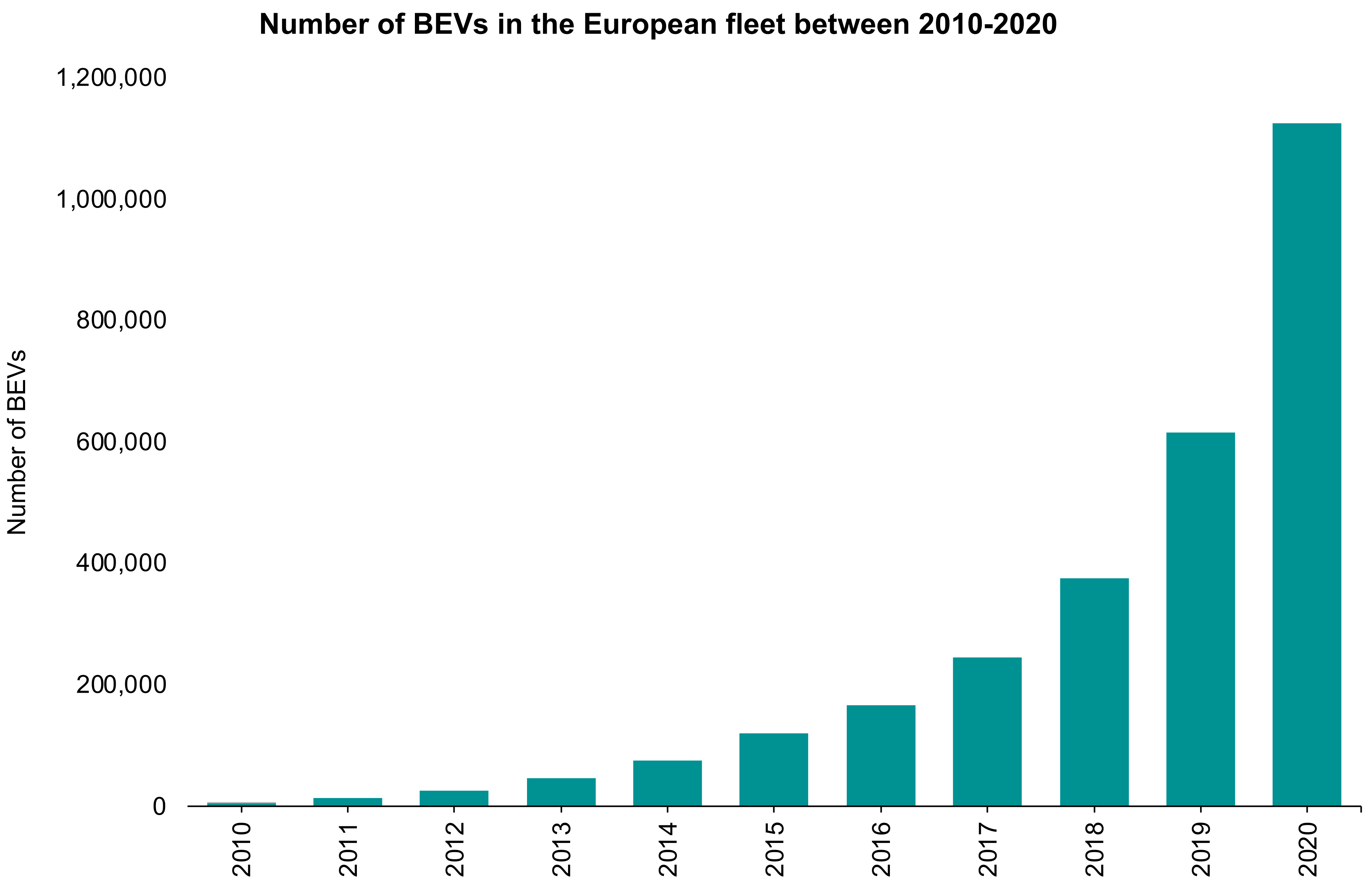
Battery Electric Vehicles (BEVs) are gradually penetrating the European market. However, despite a steady increase in the number of new electric car registrations annually, from (700) units in 2010 to about (550,000) units in 2019, they still account for a market share of only (3.5%). Moreover, the BEVs accounted for (2%) of total new car registrations in 2019, representing around two-thirds of electric car sales, while plug-in hybrid electric vehicles (PHEVs) represented (1%). Nevertheless, there was a notable increase of (129%) in new BEVs registrations between 2018 and 2019 in Europe. Indeed, this increase could be explained by the inclusion of Norway in the dataset in 2019. The country registered around (60,000) BEVs in 2019 [1]. Indeed, in Europe, the number of BEVs in the fleet in 2010 was (5785), and in 2020 it reached (1,125,484) (see Figure 1 below).

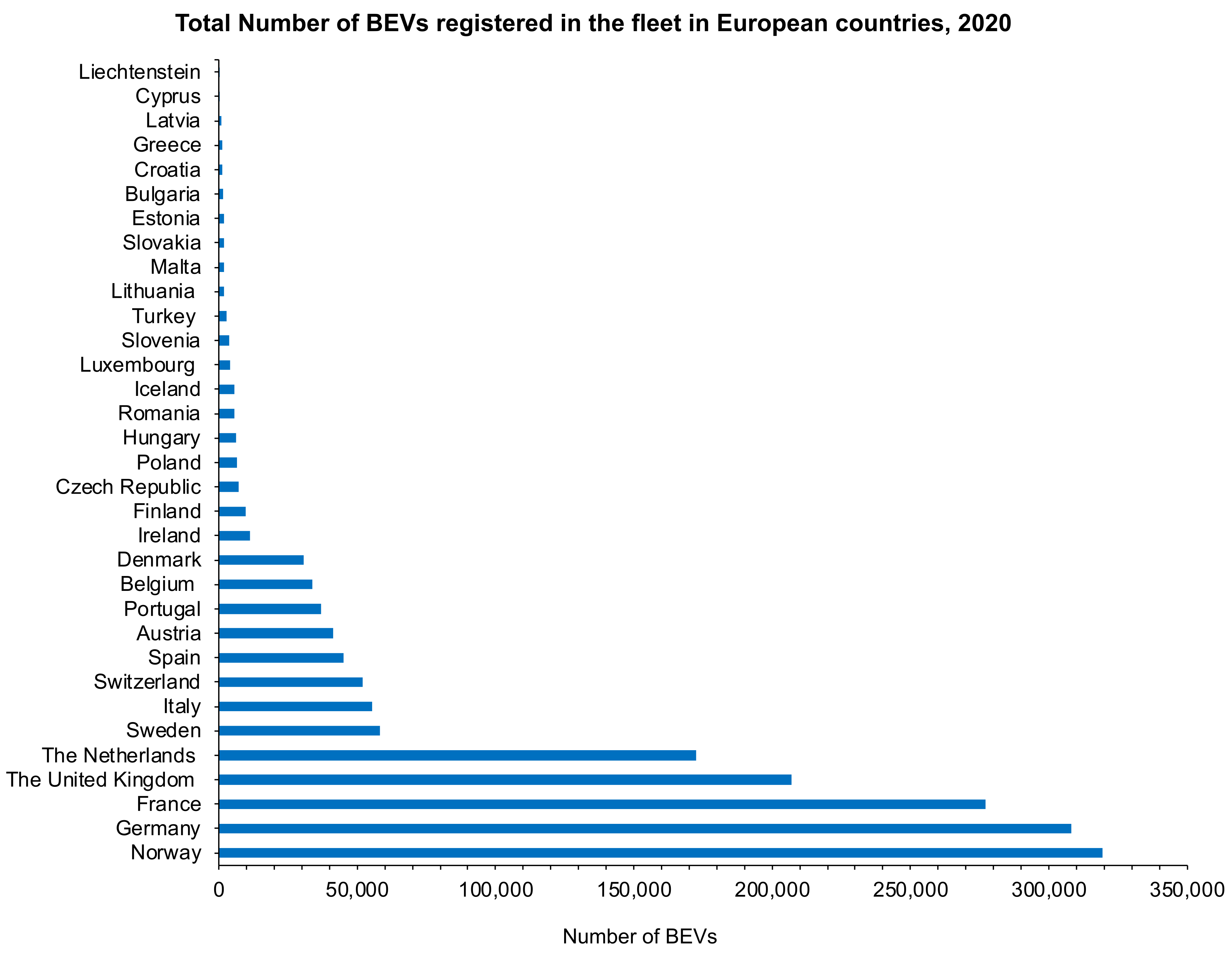
Moreover, Norway, Germany, France, the United Kingdom, and the Netherlands are the top five countries with a significant number of BEVs registered in Europe. At the same time, Liechtenstein, Cyprus, and Latvia have fewer BEVs in the fleet (see Figure 2 below).

As shown in Figure 2 above, in Norway, the number of BEVs registered in the fleet in 2020 was (319,540). In Germany, it was (308,139); in France, (277,001); in the United Kingdom, (206,998), and in the Netherlands it was (172,534). However, some countries in Europe have a low number of BEVs in their fleet; for example, Liechtenstein (222), Cyprus (251), and Latvia (846). Indeed, Germany, France, and the Netherlands accounted for about (50%) of BEVs registrations. Meanwhile, the numbers almost doubled in Germany and tripled in the Netherlands compared with 2019. Moreover, the average mass of BEVs increased from 1200 kg in 2010 to 1700 kg in 2019, while average energy consumption decreased from 264 to 150 Wh/km, indicating that BEVs have become more efficient [1]. In addition, the leading countries in electric mobility offer financial incentives such as tax reductions and exemptions for electric vehicles, designed to make the costs comparable to those of conventional vehicles [1]. Therefore, it is logical to associate the growth in the use of electric vehicles with an increase in the demand for electric energy.

However, the forecast is that total electricity consumption in Europe by electric cars will gradually grow to approximately (9.5%) by 2050 [6]. This issue resulted in some advantages; for example, a global reduction in carbon dioxide emissions (CO₂) and other air pollutants and CO₂ emissions from the transport sector. Eventually, some disadvantages include increased emissions associated with electricity production [6] regarding the energy consumption in Europe. As we already know, the final energy consumption amounted to 935 million tons of oil equivalent (Mtoe) in 2019, 0.5% less than in 2018 [7].

Therefore, the final energy consumption slowly increased from 1994 until it reached its highest value of 990 Mtoe in 2006. However, by 2019 final energy consumption decreased from its peak level by (5.5%). Indeed, this decrease is related to the financial and economic crisis. Therefore, between 1990 to 2019, the amount and share of fossil fuels dropped significantly. In 1990, their share was (9.6%) and reached a value of (3.6%) in 2000, (2.8%) in 2010, and (2.1%) in 2019 [7]. Instead, the renewable energy sources increased their share in the energy matrix. They moved from (4.3%) in 1990 to (5.3%) in 2000, (8.8%) in 2010, and reached (10.9%) in 2019. On the other hand, natural gas remained stable between 1990 and 2019, ranging from (18.8%) in 1990 to (22.6%) in 2010, reaching (21.3%) in 2019. Moreover, the oil and petroleum products had the most significant share of the energy matrix in 2019, with participation of (37%), electricity (22.8%), natural gas (21.3%), and solid fossil fuels (2.1%) to the final energy consumption [7].

Indeed, when addressing the final energy consumption per capita in European countries, we found that Luxembourg, Finland, and Iceland reached over 6 tons of oil equivalent (toe) per capita. In contrast, Romania and Malta reached under two toes per capita, and the European stood at 3.3 toes per capita in 2019 [7]. However, this could be an indicator (i) of the industry structure in each country, (ii) the severity of winter weather in the case of Iceland and Finland, and (iii) other factors, such as fuel tourism, in the case of Luxembourg [7].

In Europe, most of the energy consumption comes from the transport sector (30.9%), as well as from households (26.3%) and industry (25.6%) in 2019 [7]. The total energy consumption of all modes in Europe reached a value of 289 Mtoe in 2019. There was a marked change in the development of energy consumption for the transport sector after 2007 [7]. Indeed, until that year, the consumption of energy from the transport sector was characterized by steady growth, rising each year. However, with the onset of the global financial and economic crisis in 2008 and the European debt crisis between 2011–2013, the energy consumption from the transport sector fell (−1.4%). Moreover, this decline intensified in 2009, with reductions of (−2.5%), 2010 (−0.2%), 2011 (−0.3%), 2012 (−3.5%), and 2013 (−1.3%). In 2014, this trend reversed, and the increase in energy consumption by the transport sector continued all the way. In 2017 an increase of (+0.6%), 2019 (+1.0%), and 2019 (+2.0%) was registered, although the 2007 levels were not reached [7].

As it is already known, several drives exist that increase the consumption of energy, such as economic growth, urbanization, globalization, trade, and transportation, which are widely explored by the literature. This investigation opted to study the effect of the transport sector, more precisely the electric cars sector, on energy consumption in the European countries due to the fast growth of this sector in the last ten years. As mentioned before, the BEVs accounted for a market share of only (3.5%) of newly registered passenger vehicles. However, they accounted for (2%) of total new car registrations in 2019, representing around two-thirds of electric car sales. Therefore, despite the small participation of BEVs in the fleet, it is interesting to identify whether this sector increases energy consumption [7].

In the literature, the impact of BEVs on energy consumption is more focused on the engineering field, where several authors approached this topic (e.g., Fuinhas et al. [8]; Teixeira and Sodré [9]; Sriwilai et al. [10]; Wu et al. [11]; Dias et al. [12]; Baran and Loureiro [13]; Helmers and Marx, [14]; Vliet et al. [15]; Salihi [16]). For example, Teixeira and Sodré [9] evaluated the impacts on energy consumption and carbon dioxide (CO₂) emissions from introducing electric vehicles into a smart grid. The AVL Cruise software was used to simulate two cars, one electric and the other engine-powered, both operating under the New European Driving Cycle (NEDC), to calculate CO₂ emissions, fuel consumption, and energy efficiency. The authors found that CO₂ emissions from an electric vehicle fleet can be 10 to 26 times lower than that of an engine-powered vehicle fleet. In addition, the scenarios indicate that even with high factors of CO₂ emissions from energy generation, significant reductions in annual emissions are obtained with the introduction of electric vehicles in the fleet. Sriwilai et al. [10] simulated the effect of electric cars on energy consumption in Thailand using ANFIS. The simulation results indicated that a personal electric vehicle could gasoline consumption reduce to 2189 liters per year, but an electric taxi can reduce gas consumption by 10,515 liters per year. Wu et al. [11] measured electric vehicles’ energy consumption. The analysis shows that energy consumption is more efficient and consumes less when driving on city routes than when driving on freeways.

Therefore, there is a lack of literature that addresses the effect of BEVs on energy consumption using an econometric approach and macroeconomic data and, more precisely, the European countries. Furthermore, this investigation takes a vital role regarding the effect of electric cars on energy consumption in the literature.

Faced with a lack of literature regarding the impact of BEVs on energy consumption using a macroeconomic and econometric approach, we carry out the following question—What is the impact of battery-electric vehicles on energy consumption in the European countries? This investigation will conduct an empirical analysis using macroeconomic panel data with twenty-nine countries from the European region between 2010 and 2020 to answer this question. This investigation will use the quantile regression model (QRM) and ordinary least squares (OLS), with fixed effects as methods.

This investigation will contribute to the literature for several reasons: first, it will introduce a new analysis related to the effect of BEVs on energy consumption using a macroeconomic and econometric analysis. This kind of investigation is not explored by economists and can open new opportunities to study this topic using data analysis and econometrics. Second, this investigation will contribute to the introduction of econometric models (e.g., QRM and OLS with fixed effects) that are not studied by literature on this topic. Third, the introduction of new variables, such as E-commerce in econometric models, explains energy consumption in European countries. This variable was not explored before in the literature.

Moreover, this investigation is essential because it will help governments and policymakers develop more initiatives to promote BEVs in the European countries and mechanisms and policies to reduce energy consumption by increasing energy efficiency. All this will mitigate energy consumption from non-renewable energy sources and environmental degradation. Finally, this investigation also can open a new channel of policy discussion between industry, government, and researchers, as a crucial step towards ensuring that BEVs provide a climate change mitigation pathway in the region.

This study is organized as follows. Section 2 presents the literature review. Section 3 provides the data and the method approach. Section 4 presents the results. Section 5 presents the discussions. Section 6 presents the conclusions and policy implications. Finally, Section 7 reveals the limitations of the study.

2. Literature Review

This section is divided into two main subsections. Section 2.1 will approach the studies that conducted the effect of electric vehicles on energy consumption, while Section 2.2 will approach the effect of GDP and e-commerce on energy consumption.

2.1. The Effect of Electric Vehicles on Energy Consumption

Several authors have explored the impact of electric vehicles on energy consumption. However, most of them are related to the engineering areas. New authors from social sciences or economics have explored this relationship. From these few authors, this investigation can highlight that Fuinhas et al. [8] explored the effect of BEVs on greenhouse gas emissions (GHGs) in 29 European Union Countries macroeconomically. The authors found that the BEVs can mitigate GHG emissions. However, this reduction is related to the capacity of BEVs consuming less energy. Indeed, in their additional analysis, the authors found that BEVs can reduce energy consumption by (−0.0154). Moreover, this reduction is related to increasing energy efficiency in electric vehicles.

This idea aligns with the vision of the European Environment Agency [1] and Nielsen and Jørgensen [17]. According to Nielsen and Jørgensen [17], BEVs’ energy consumption will be 0.10 (kWh/km) between 2016 and 2030. Other authors from engineering areas also mentioned that the BEVs consume less energy than alternatives. For example, Teixeira and Sodré [9] evaluated the impacts on energy consumption and carbon dioxide (CO₂) emissions from introducing electric vehicles into a smart grid. The AVL Cruise software was used to simulate two vehicles, one electric and the other engine-powered, both operating under the New European Driving Cycle (NEDC), to calculate CO₂ emissions, fuel consumption and energy efficiency. The authors found that CO₂ emissions from the electric vehicle fleet can be 10 to 26 times lower than that of the engine-powered vehicle fleet. In addition, these scenarios indicate that even with high factors of CO₂ emissions from energy generation, significant reductions in annual emissions are obtained with the introduction of electric vehicles in the fleet. Additionally, Sobol and Dyjakon [18] found that indirect CO₂ associated with the daily driving of electric vehicles is higher than direct emissions associated with internal combustion engines usage in Poland.

Sriwilai et al. [10] simulated the effect of electric cars on energy consumption in Thailand using ANFIS. The simulation results indicated that a personal electric car could reduce gasoline consumption to 2189 liters per year, but an electric taxi can reduce gas consumption by 10,515 liters per year. Wu et al. [11] measured electric vehicles’ energy consumption, and the analysis showed that energy consumption is more efficient and consumes less when driving on city routes than freeways. Finally, Helmers and Marx [14] explored the effect of electric cars on the environment. The authors found that this kind of vehicle can mitigate environmental degradation due to its capacity to consume less energy.

Holmberg and Erdemir [19] investigated the impact of tribology on energy use and CO₂ emissions. They showed that total energy use in battery-powered electric passenger cars is on average 3.4 times lower compared to combustion engine-powered cars. However, the CO₂ emissions are 4.5 times higher for a combustion engine car than an electric car when the electricity comes from renewable energy sources. Additionally, moving from fossil to renewable energy sources may cut down the energy losses due to friction in energy production by more than (60%).

However, other authors that also investigated this topic found that electric cars can increase energy consumption, such as Dias et al. [12], who found that a (10%) increase of electric cars in the fleet corresponds to an increase of (2%) of the electricity demand in São Paulo (Brazil). In addition, Baran and Loureiro [13] studied the impact of electric vehicles on energy consumption in Brazil. The authors also found that electric cars also increase energy consumption. According to the authors, electric cars can increase electricity consumption by (31.3%).

Since most previous studies ignore distribution heterogeneity, this study examines distribution heterogeneity using panel quantile regression. It can be noted that the novelty of this study in comparison with other studies performed in European countries is that the panel quantile regression method was not used to investigate the effect of battery electric vehicles on energy consumption in any of the studies. Additionally, a study has not yet examined the impact of electric cars, economic growth, and e-commerce on energy consumption in European countries.

2.2. The Effect of Gross Domestic Product (GDP) and E-Commerce on Energy Consumption

Several authors have exhaustively explored the impact of economic growth on energy consumption (e.g., Fuinhas et al. [8]; Koengkan and Fuinhas [20]; Buhari et al. [21]; Wang et al. [22]; Shahbaz et al. [23]; Saidi and Hammami [24]; Komal and Abbas [25]; Nasreen and Anwar [26]). For example, Fuinhas et al. [8] investigated the effect of BEVs on GHGs in 29 European Union Countries macroeconomically. The authors found that economic growth increases energy consumption in (0.4667). Koengkan and Fuinhas [20] examined the impact of the obesity problem on energy consumption in thirty-one countries from Europe between 1990 to 2016. The authors used the quantile via moments approach as a method. The authors found that the GDP per capita increases the energy consumption per capita. Buhari et al. [21] explored the nexus between non-renewable and renewable energy consumption and economic growth. They considered the moderating impact of economic complexity, trade openness, Foreign direct investment (FDI) and institutional quality using a panel quantile regression model and data from 32 European countries from 1995 to 2014. The authors found that the economic complexity, renewable energy consumption, trade openness, FDI, and institutional quality enhance economic growth. Moreover, results for non-renewable energy consumption showed both a positive and a negative impact in different quantiles, indicating that renewable energy consumption is, in fact, more effective for economic growth than non-renewables.

Wang et al. [22] evaluated the effects of urbanization, energy prices, and economic growth on energy consumption in three country groups (high-income, upper- and lower-middle-income). The results indicated a positive relationship between GDP and energy consumption in all three groups. Shahbaz et al. [23] empirically investigated the inter-linkages between energy consumption and economic growth in the top ten energy-consuming countries (e.g., China, the USA, Russia, India, Japan, Canada, Germany, Brazil, France, and South Korea). As a method, the authors used the quantile-on-quantile (QQ) approach. The authors found a positive association between economic growth and energy consumption, with considerable variations across economic states in each country. A weak effect of economic growth on energy consumption is noted for the lower quantiles of economic growth in China, India, Germany and France, which suggests that energy as an input has less importance at low levels of economic growth. A weak effect of economic growth on energy consumption is also noted for the highest quantiles of income in the United States, Canada, Brazil, and South Korea. This result indicates that energy demand decreases with economic growth as these countries have become more energy efficient.

Saidi and Hammami [24] studied the impact of economic growth on energy consumption for a global panel of 58 countries from 1990 to 2012. The authors found that the impact of economic growth on energy consumption is positive. Komal and Abbas [25] examined the linking financial development, economic growth and energy consumption in Pakistan between 1972 and 2012. The authors used the generalized method of moments (GMM). The authors found a positive and significant impact of economic growth and urbanization on energy consumption, while the effect of energy prices over energy consumption is significant but negative. Finally, Nasreen and Anwar [26] investigated the causal relationship between economic growth, trade openness, and energy consumption using data from 15 Asian countries between 1990 and 2011. The authors used the panel cointegration and causality approaches to examine the long-run and causal relationship between variables. The empirical results indicated the positive impact of economic growth and trade openness on energy consumption.

Ben-Jebli and Hadhri [27] showed bidirectional causality between economic growth and energy use using the vector error correction model and Granger causality test approach. They applied combined panel data techniques with wavelet spectral analysis for the 50 states of the USA from 1963–2017. Saldivia et al. [28] concluded that there is evidence for the direction of causality between energy consumption and GDP in the short run. However, most subgroups have bidirectional causality between energy consumption and GDP in the medium- and long-run.

The impact of e-commerce on energy consumption has seldom been explored in the literature. However, some authors investigated this topic issue (e.g., Dost and Maier [29]; Pålsson et al. [30]; Williams and Tagami [31]; Matthews et al. [32]; Hidayatno et al. [33]; Weber et al. [34]; Cholette and Venkat [35]; and Stinson et al. [36]).

Indeed, some identified that e-commerce increases energy consumption (e.g., Dost and Maier [29]; Pålsson et al. [30]; Williams and Tagami [31]; Matthews et al. [32]; and Hidayatno et al. [33]). For example, Dost and Maier [29] examined the relationship between e-commerce and energy consumption in the US economy during 1992–2015. The results show that e-commerce increases energy consumption through increases in the commercial and residential sectors. Pålsson et al. [30] analyzed the impact of conventional trade with stores or e-commerce, with home delivery being deemed more energy efficient. The authors found that e-commerce increases energy consumption. Williams and Tagami [31] investigated the impact of e-commerce and conventional retail in energy use in Japan. The authors found that e-commerce uses more energy per book than conventional retail in dense urban areas because of additional packaging. However, in suburban and rural areas, the energy consumption of the two systems is nearly equal because the relative efficiency of courier services compared to personal automobile transport balances out the impact of additional packaging. The main reason e-commerce does not save energy, even in rural areas, is the multipurpose use of automobiles; e-commerce consumes less energy in the case of single-purpose shopping trips by automobile.

Matthews et al. [32] analyzed the different logistics networks and assessed different delivery systems’ energy and cost impacts in the United States and Japan. The results suggest a crossover in energy use according to population density in Japan. In the United States, a crossover also exists based on the delivery method and distance to local bookstores. However, in neither case are the potential spillovers energy benefits from e-commerce-based methods considered. The results showed notable differences for the two distribution methods and suggested areas where further energy improvements may be possible. Using Model Conceptualization, Hidayatno et al. [33] showed that the rise of e-commerce in urban areas has changed the way people buy goods, leading to higher delivery frequencies in urban areas, which leads to more energy consumption CO₂ emissions in Jakarta.

However, other authors found that e-commerce reduces energy consumption (e.g., Weber et al. [34]; Cholette and Venkat [35]; Stinson et al. [36]). For example, Weber et al. [34] studied the impact of traditional retail or e-commerce sales of compact discs or a digital download service on energy and CO₂ emissions. The authors analyzed a set of six (three compact discs and three digital downloads) scenarios for the delivery of one music album from the recording stage to the consumer’s home in either CD or digital form. The authors found that despite the increased energy and emissions associated with Internet data flows, digitally purchasing music reduces the energy and CO₂ emissions associated with delivering music to customers by between (40%) and (80%) from the best-case physical CD delivery, depending on whether a customer then burns the files to CD. Cholette and Venkat [35] investigated the impact of logistical options for delivering wine to consumers on energy consumption and CO₂ emissions. The authors found that the e-commerce option consumes less energy than traditional retail. Stinson et al. [36] indicated that E-commerce had increased the parcel truck delivery trips. The net effect of e-commerce is to reduce fuel consumption due to a significant reduction in these amounts through shopping trip reductions.

This section presented a brief literature review regarding the impact of electric vehicles, GDP, and e-commerce on energy consumption. The following section will be present the data and method.

3. Data and Method

This section will show a group of countries, data/variables, and methods used in this investigation.

3.1. Data

The data from 2010 to 2020 were collected for a group of twenty-nine countries from the European region (e.g., Austria, Belgium, Bulgaria, Croatia, Cyprus, Czechia, Denmark, Estonia, Finland, France, Germany, Greece, Hungary, Iceland, Ireland, Italy, Latvia, Lithuania, Luxembourg, Norway, the Netherlands, Poland, Portugal, Romania, Slovakia, Slovenia, Spain, Sweden, and the United Kingdom). Indeed, this investigation selected 29 European countries to carry out this analysis for several reasons. First, the increase in BEVs in the fleet in all 29 European countries, as mentioned in the introduction section. Second, technical issues, as the Quantile regression model (QRM) requires the N > T. The variables chosen to perform this investigation will be shown in

Table 1. Variables’ description.

Dependent Variables
Variable	Description	Time	Source
ENERGY	Final energy consumption, in thousand tons of oil equivalent, per capita. Indeed, this variable covers the energy consumption from industry, transport, households, services, and agriculture sectors and excludes the consumption from the energy sector itself and losses occurring during the transformation and distribution of energy (e.g., power plants, district heating plants, oil refineries, coke ovens, blast furnaces). Moreover, it also excludes all non-energy use of energy carriers (e.g., natural gas used for producing chemicals, oil-based lubricants, bitumen used for road surface).	2010–2020	Eurostat [37]
Independent variables
GDP	GDP per capita based on purchasing power parity (PPP). PPP GDP is gross domestic product converted to international dollars using purchasing power parity rates.	2010–2020	World Bank Open Database [38]
E-COMMERCE	Percentage of individuals who used the internet to purchase online within the last year.	2010–2020	Eurostat [37]
BEV	The number of battery electric vehicles (BEV) registered in the fleet. A battery-electric vehicle, pure electric vehicle, only electric vehicle, or all-electric vehicle is an electric vehicle that exclusively uses chemical energy stored in rechargeable battery packs, with no secondary source of propulsion.	2010–2020	European Alternative Fuels Observatory (EAFO) [5]

below.

The variable ENERGY is the dependent variable, while the variables GPD, E-COMMERCE, and BEV are the independent variables. Therefore, the variables GDP and E-COMMERCE are the control variables of the empirical model. Furthermore, the variable ENERGY as a dependent variable was used by several authors (e.g., Buhari et al. [21]; Wang et al. [22]; Saidi and Hammam [24]; Dost and Maier [29]). The same occurs with the variable GDP, which also is widely used by literature as an independent variable to explain the increase in energy consumption (e.g., Buhari et al. [21]; Wang et al. [22]; Shahbaz et al. [23]; Dost and Maier [29]; and Pålsson et al. [30]). However, only the variables BEVs and E-COMMERCE were not approached by the literature to explain the energy consumption in a macroeconomic and econometric context. Therefore, as this investigation has three variables that were not approached by econometric and macroeconomic literature, this investigation does not follow a developed conceptual framework. Moreover, all variables are in natural logarithms (e.g., LnENERGY, LnGDP, LnE-COMMERCE, and LnBEV) to harmonize the interpretation of results and linearize the relationships between variables.

3.2. Method

The methods QRM and OLS with Fixed Effects and the statistical tests used will be presented in this subsection.

3.2.1. Quantile Regression Model (QRM)

As mentioned in the data section, this research investigates the impact of battery electric vehicles on energy consumption in twenty-nine European countries. In this regard, this study performed the QRM and OLS with fixed effects. QRM is one of the most popular applied econometrics models introduced by Koenker and Bassett [39]. This model considers the unobserved heterogeneity and heterogeneous covariates. It also determines the fixed effects for controlling the unobserved covariates at different quantiles [8]. The typical definition of QR can be presented as the following (Equation (1)):

$$Quan{t}_{\tau } \left(\left.y_i\right|x_i\right)=x{\beta }_{\tau }+u_{\tau } , 0<\tau <1,$$

(1)

where y presents the endogenous variable; x refers to the independent variables. The error term in the $\tau$-th distribution point of the dependent variable is defined by $u$ [40]. In a simple way, the model presented in this research is computed as follows:

$$\begin{gathered} LnENERG{Y}_{it}={\beta }_0+{\beta }_{1}LnGD{P}_{it}+{\beta }_{2}LnE\_COMMERC{E}_{it}+{\beta }_{3}LnBE{V}_{it}+{\epsilon }_{it} \\ as \to i=1\dots 28; t=2010\dots 2020 \end{gathered}$$

(2)

where $LnENERG{Y}_{it}$ refers to the dependent variable to estimate energy consumption for each country in the panel data model. The independent variables (explanatory variables) are $LnGD{P}_{it}$, $LnE\_COMMERC{E}_{it}$, and $LnBE{V}_{it}$ (refer to all the independent variables; see Table 1). The error term in the t-th distribution point of the dependent variable is denoted by $\epsilon$ [41]. In addition, the β₁, β₂, and β₃ coefficients are to be computed, and ${\beta }_0$ states the model intercept. In Equation (1), the description of each variable is denoted in Table 1.

3.2.2. Ordinary Least Squares (OLS) with Fixed Effects

The OLS with fixed effects estimated the intercepts and slope for a set of observations. Moreover, this method also can estimate the fixed predictors using the conditional mean function (see Equation (3), below).

$$LnENERG{Y}_{it}={\beta }_0+{\beta }_{1}LnGD{P}_{it}+{\beta }_{2}LnE\_COMMERC{E}_{it}+{\beta }_{3}LnBE{V}_{it}+{\epsilon }_{it}$$

(3)

where β₀ is the intercept and β is the value of fixed covariates being fitted to predict the dependent variable LnENERGY_it; ε_i is the error term, and each variable enters regression for country i at year t.

3.2.3. Statistical Tests

A few tests can be applied to select the most appropriate model and trace the adequate computation method. In this research, the following tests listed in

Table 2. Preliminary tests for the fixed effects that are used in this study.

Test	Reference	Description
Hausman	Hausman [42]	This test checks the presence of random effects vs. fixed effects; Identifies heterogeneity.
Panel Unit Root test (CIPS)	Pesaran [43]	This test identifies the presence of unit roots.
Cross-sectional dependence (CD)	Pesaran [44]	This test checks the presence of cross-sectional dependence in the model.
Shapiro-Wilk	Shapiro and Wilk [45]	This test checks the presence of normality of the panel model.
Skewness/Kurtosis	D’Agostino et al. [46]	This test checks the presence of normality.
Variance Inflation Factor (VIF)	Belsley et al. [47]	This test checks the presence of multicollinearity in the model
Westerlund panel cointegration	Westerlund [48]	This test checks the presence of cointegration

Notes: This table was created by the authors.

are performed.

The empirical analysis was carried out using the econometric software Stata 17.0. The following section will present the empirical results of this study.

4. Empirical Results

This section will introduce the main results of this investigation.

Table 3. Descriptive statistics.

Variables	Descriptive Statistics
	Obs.	Mean	Std.-Dev.	Min.	Max.
LnENERGY	319	−5.3818	0.4407	−6.1119	−4.0517
LnGDP	319	10.5826	0.3718	9.7665	11.6434
LnE-COMMERCE	319	3.9791	0.4272	2.1972	4.5108
LnBEV	319	5.4540	2.9616	0.0000	12.1417

provides the first insight into the variables and descriptive statistics of variables. The Obs. denotes the number of observations in the model. Std.-Dev. denotes the Standard Deviation. Min. and Max. denote Minimum and Maximum. The Stata command sum was used. Moreover, (Ln) means variables in the natural logarithms.

The variables are presented in natural logarithms, and the number of observations in Table 3 above points to the presence of a balanced panel. The Skewness and Kurtosis test described by D’agostino et al. [46] and the Shapiro–Wilk test [45], extended by Royston [49], is used to check the normality of the data. The results of the Normal distribution test are presented in

Table 4. Normal distribution tests.

Variables	Obs.	Skewness	Kurtosis	Skewness/Kurtosis Tests		Shapiro-Wilk Test
				Prob > Chi2		Prob > z
LnENERGY	319	0.0000	0.0008	0.0000	***	0.0000	***
LnGDP	319	0.0012	0.1641	0.0039	**	0.0000	***
LnE-COMMERCE	319	0.0000	0.0002	0.0000	***	0.0000	***
LnBEV	319	0.2871	0.0018	0.0072	**	0.0002	***

Notes: ***, **, denote statistically significant at (1%) and (5%) level.

below. The Stata commands sktest and swilk were used in these tests.

The evidence rejects the null hypothesis of normally distributed data of the Skewness and Kurtosis test at (1%) and (5%) significance levels. Moreover, the Shapiro–Wilk rejects the null of normal distribution for all variables in the model at a (1%) significance level, therefore pointing to non-normal distributed data. The Variance Inflation Factor (VIF) test [47] was calculated to detect multicollinearity in the model regression. A considerable value for VIF indicates the existence of low multicollinearity between the variables. The results of the VIF-test are shown in

Table 5. VIF-test.

Variables	VIF	1/VIF	Mean VIF
LnENERGY
LnGDP	2.02	0.4957	2.33
LnE-COMMERCE	2.97	0.3368
LnBEV	2	0.4992

. The Stata command vif was used in this test.

The VIF test suggests no multicollinearity concerns since VIF is inferior to the critical value of 10 (2.97 being the highest), and the Mean VIF has a low value. When handling panel data, it is necessary to check the presence of cross-sectional dependence (CDS). The cross-sectional dependence (CSD) test of Pesaran [44] has a null hypothesis of cross-sectional independence, and the error term is independent and identically distributed across time and cross-sections.

Table 6. Pesaran CD-test.

Variables	CD-Test	p-Value
LnENERGY	19.26	0.000	***
LnGDP	47.10	0.000	***
LnE-COMMERCE	58.74	0.000	***
LnBEV	58.79	0.000	***

Notes: *** denotes statistically significant at (1%) level.

below presents the results from the CD-test. The Stata command xtcd was used in this test.

Findings in Table 6 illustrate that the null is rejected at a (1%) significance level for all the variables in natural logarithms. Therefore, the presence of cross-sectional dependence is expected. This result is due to common factors shared by European countries that are unobserved (or unobservable). Thus, further tests and estimation techniques need to account for CSD.

Following the previous reasoning, a second-generation unit root test was employed to determine the presence of unit roots in the variables under the nonstationary null. The Stata command multipurt was used in this test. The results of the CIPS test [43] are shown in

Table 7. Unit Root test.

Variables	Panel Unit Root Test (CIPS) (Zt-Bar)
	Without Trend			With Trend
	Lags	Adjusted t		Adjusted t
LnENERGY	1	1.941		−3.880	***
LnGDP	1	−1.586	***	−3.458	***
LnE-COMMERCE	1	−3.311	**	−3.392	**
LnBEV	1	0.196		−0.291	*

Notes: ***, **, * denotes statistically significant at (1%), (5%), and (10%) level.

and support that, without and with a time trend, LnGDP and LnE-COMMERCE are stationary at (1%) and (5%) significance levels, respectively. The null is not rejected for LnENERGY and LnBEV without the time trend while rejected at (1%) and (10%) significance level with the time trend, respectively. The variables LnENERGY and LnBEV are quasi-stationary, that is, on the boundary between the I(0) and I(1) order of integration.

Therefore, cointegration analysis is required. The Westerlund panel cointegration test [48] tests the null hypothesis of no cointegration by testing if the conditional panel error-correction term equals zero [50]. Gt and Ga are group-mean tests, meaning that both test cointegration for each country individually, and Pt and Pa are panel tests that test cointegration of the panel. Moreover, the Westerlund test requires that the variables be stationary, as Koengkan et al. [51] mentioned. In the case of this investigation, only the variables LnGDP and LnE-COMMERCE are stationary. That is, the test can be computed only for these two variables. However, the variables LnENERGY and LnBEV were not used in this test because they are quasi-stationary. In other words, these variables are on the borderline between the I(0) and I(1) order of integration. The results of the Westerlund test are shown in

Table 8. Westerlund panel cointegration test.

Variables LnGDP and LnE-COMMERCE
Statistic	Value	Z-Value	p-Value
Gt	−1.421	2.140	0.984
Ga	−3.488	3.615	1.000
Pt	−7.119	0.681	0.752
Pa	−5.235	−1.219	0.111

Notes: denotes statistically significant at (1%) level. H0: No cointegration; H1 Gt and Ga test the cointegration for each country individually, and Pt and Pa test the cointegration of the panel.

. The Stata command xtwest with option constant was used in this test.

Table 8 above shows that the null hypothesis should not be rejected and, therefore, there is no cointegration. The Hausman test [42] allows the most appropriate estimator to be chosen. The null hypothesis of the Hausman test is that the unique errors are not correlated with the regressors or, in other words, that the difference in coefficients is not systematic. In short, accepting the null favors random effects over fixed effects. The sigmaless option specifies that the covariance matrices are based on the consistent estimator’s estimated disturbance variance.

Table 9. Hausman test.

Dependent Variable LnENERGY
Variables	(b) Fixed	(B) Random	(b-B) Difference	Sqrt(diag(V_b-V-B)) S.E.
LnGDP	0.4188	0.4535	−0.0347	0.0108
LnE-COMMERCE	0.0214	0.0203	0.0011	0.0018
LnBEV	−0.0146	−0.0153	0.0007	0.0001
Chi2 (3)	15.91 ***

Notes: *** denotes statistically significant at the (1%) level.

presents the results of the Hausman test. The Stata command hausman (with the options, sigmaless) was used in this test.

The null hypothesis is rejected in this study at (1%) significance levels, concluding that the internal estimator better suits the empirical model of this investigation.

Table 10. Results from QRM and OLS with fixed effects.

Independent Variables	Dependent Variable (LnENERGY)
	Quantiles						OLS
	25th		50th		75th		Fixed Effects
LnGDP	0.5089	***	0.8791	***	0.9089	***	0.4188	***
LnE-COMMERCE	0.3156	***	0.2397	***	0.2362	***	0.0214
LnBEV	−0.0268	***	−0.0493	***	−0.0478	***	−0.0146	***
Constant	−12.0422	***	−15.3754	***	−15.5705	***	−9.819	***
Obs	319		319		319		319
Pseudo R2	0.3723		0.4223		0.4786		0.5850

Notes: ***, denotes statistically significant at (1%) level.

provides the regression results. The Stata commands sqreg with option reps (300) and xtreg, fe were used. This investigation employs a simultaneous-quantile regression for the 25th, 50th, and 75th quantile of the dependent variable and an OLS with fixed effects. The quantile regression has the advantage of showing the differential impact of the explanatory variables on the distribution of LnENERGY.

The results above indicate that the variables LnGDP impact positively the variable LnENERGY in the 25th, 50th, and 75th quantiles at a (1%) significance level. The former interpretation also applies to the effect of LnE-COMMERCE on LnENERGY. Thus, economic development and online commerce increase final energy consumption. On the other hand, the variable LnBEV negatively impacts the variable LnENERGY in the 25th, 50th, and 75th quantiles at a (1%) significance level, indicating that an increase in registered battery electric vehicles reduces final energy consumption. The OLS with fixed effects results shows that the variable LnGDP positively impacts the variable LnENERGY at a (1%) significance level, while the variable LnE-COMMERCE is not statistically significant. Therefore, economic development increases the final energy consumption. On the other hand, the independent variable LnBEV negatively impacts the variable LnENERGY at a (1%) significance level, this meaning that battery electric vehicles reduce final energy consumption. 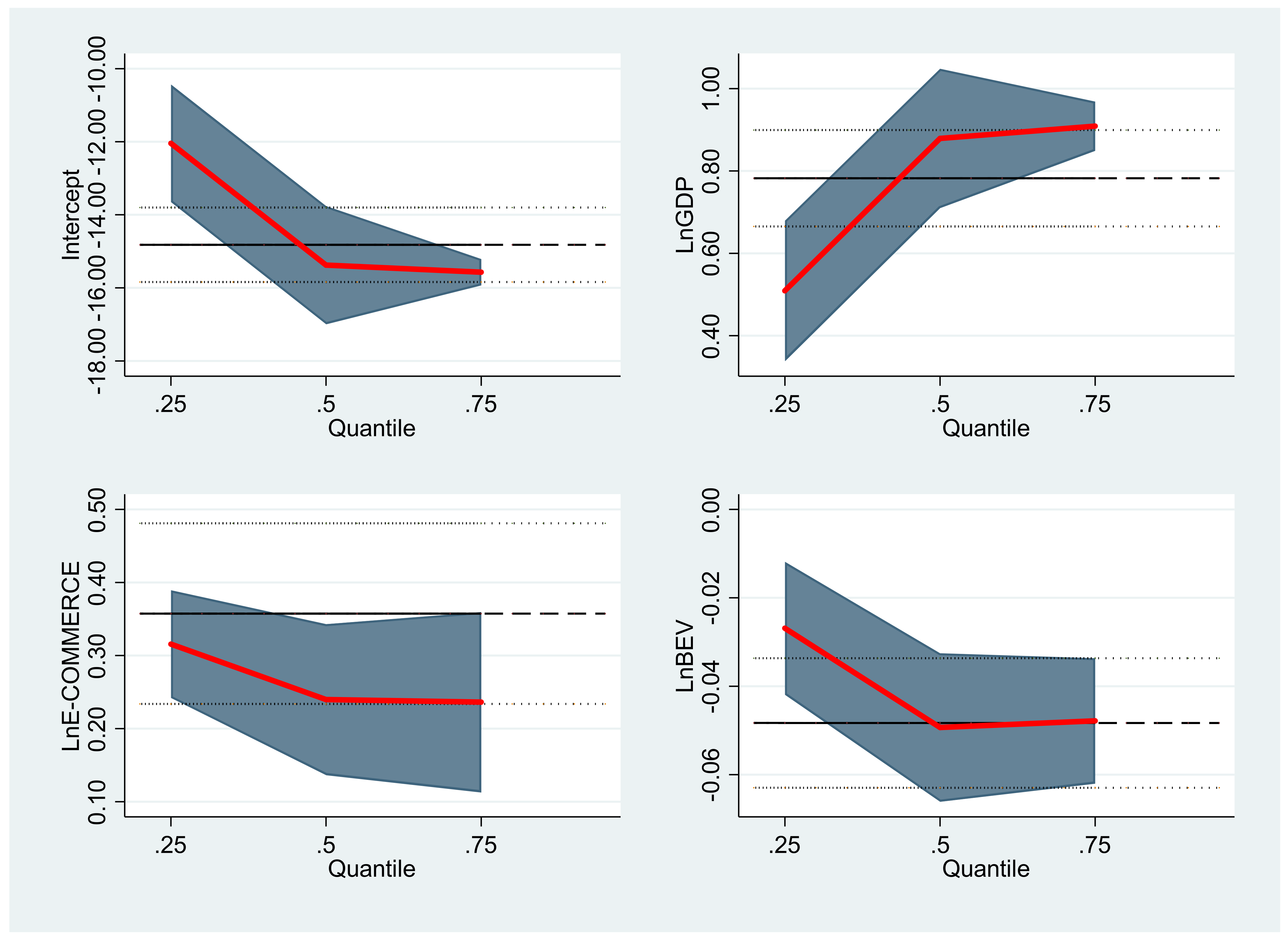Figure 3 graphically illustrates the quantile regression estimation. The vertical axis presents the estimated elasticities of the independent variables, and the horizontal lines picture the (95%) confidence intervals for the OLS coefficient.

Indeed, to identify the robustness of model regressions (e.g., QRM and OLS with fixed effects), this investigation added dummy variables to verify if the models are robust in the presence of shocks. These shocks were identified in the residuals of model regressions through visual analysis. Therefore, these dummy variables were added to the model because, during this investigation’s period (e.g., 2010–2020), the European countries suffered some shocks (e.g., economic, political, and social). However, these shocks could produce inaccurate results that lead to misinterpretations if not considered [52,53].

Indeed, before adding the dummy variables in the model regressions, it is necessary to realize a process of selection based on a triple criterion choice [52]. According to the authors, the selection of dummy variables must meet the following criteria: (a) The occurrence of international events that impacted the European region; (b) a significant disturbance in the estimated residuals; (c) the potential relevance of recorded economic, political, and social events at the country or region levels. Therefore, based on the triple criterion choice mentioned above, this investigation added the following dummy variables: IDEUROPE_2012 (shock that occurred in all European countries in 2012); IDEUROPE_2013 (shock that occurred in all European countries in 2013). These two shocks mean a break in the GDP of all countries in the model. As we already know, the European countries were impacted by the European debt crisis. Indeed, several eurozone members (e.g., Cyprus, Greece, Portugal, Ireland, and Spain) could not repay or refinance their government debt. These breaks affected economic growth, consumption behavior, industrial production, and energy consumption in most countries in Europe [53].

Table 11. Results from QRM and OLS with fixed effects with dummy variables.

Independent Variables	Dependent Variable (LnENERGY)
	Quantiles						OLS
	25th		50th		75th		Fixed Effects
IDEUROPE_2012	0.0111	***	0.0303	**	0.0163	**	0.0731	**
IDEUROPE_2013	−0.0038	***	0.0074	***	0.0021	**	−0.0052	**
LnGDP	0.5024	***	0.8872	***	0.8951	***	0.4175	***
LnE-COMMERCE	0.3197	***	0.2390	***	0.2460	***	0.0228
LnBEV	−0.0270	***	−0.0488	***	−0.0462	***	−0.0146	***
Constant	−11.9878	***	−15.4640	***	−15.4751	***	−9.8122	***
Obs	319		319		319		319
Pseudo R2	0.3724		0.4229		0.4794		0.5858

Notes: ***, **, denotes statistically significant at (1%) and (5%) level.

provides the regression results with dummy variables. The Stata commands sqreg with option reps (300) and xtreg, fe were used. This investigation analysis employs a simultaneous-quantile regression for the 25th, 50th, and 75th quantile of the dependent variable and an OLS with fixed effects. The quantile regression has the advantage of showing the differential impact of the explanatory variables on the distribution of LnENERGY.

The results above indicate that the dummy variables IDEUROPE_2012 and IDEUROPE_2013 in the 25th, 50th, and 75th quantiles and the OLS model are statistically significant at the (1%) level. The results also indicated that the variable LnGDP positively impacts the variable LnENERGY in the 25th, 50th, and 75th quantiles at a (1%) significance level. The former interpretation also applies to the variable LnE-COMMERCE on variable LnENERGY. On the other hand, the variable LnBEV negatively impacts the variable LnENERGY in the 25th, 50th, and 75th quantiles at a (1%) significance level, indicating that an increase in registered battery electric vehicles reduces final energy consumption. The OLS with fixed effects results shows that the variable LnGDP positively impacts the variable LnENERGY at a (1%) significance level, while the variable LnE-COMMERCE is not statistically significant. The independent variable LnBEV negatively impacts the variable LnENERGY at a (1%) significance level, meaning that battery electric vehicles reduce final energy consumption. 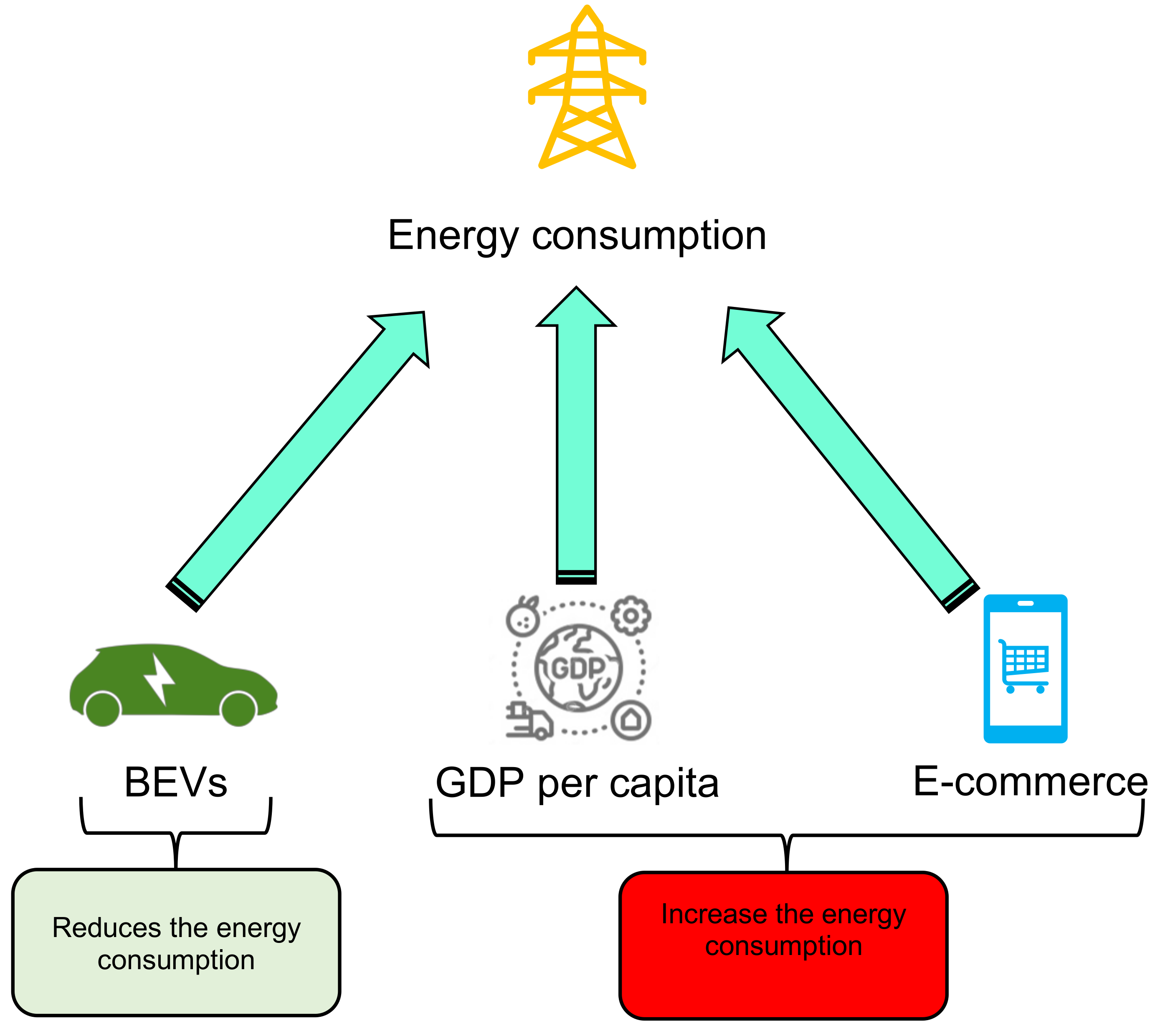The results showed in Table 11 are robust in the presence of shocks in the model, where the results had little variation compared to the results from Table 10. Therefore, this confirms that the method approach and variables used in this analysis are correct. Moreover, Figure 4 below summarizes the impact of independent variables on dependent ones. This figure was based on results from Table 10 and Table 11.

This section presented the results from the preliminary tests and the empirical results. The following section will present the discussions and present the possible explanations for the results found.

5. Discussions

This section will address the discussions of results found in this empirical investigation. As shown in Section 4, the variables LnGDP and LnE-COMMERCE positively impact variable LnENERGY, i.e., increase the energy consumption in the European countries, while the variable LnBEV reduces. In light of these findings, this investigation presented the following question: What are the possible explanations for the empirical results found? Finally, this investigation will explain macroeconomically the results found.

Therefore, the positive impact of GDP per capita on energy consumption was found by several authors (e.g., Fuinhas et al. [8]; Koengkan and Fuinhas [18]; Buhari et al. [21]; Wang et al. [22]; Shahbaz et al. [23]; Saidi and Hammami [24]; Komal and Abbas [25]; and Nasreen and Anwar [26]). According to Fuinhas et al. [8], the positive impact of GDP per capita on energy consumption is related to the European economies’ growing energy consumption dependence. This vision is shared with several authors (e.g., Koengkan and Fuinhas [18]; Buhari et al. [21]; Wang et al. [22]; Shahbaz et al. [23]; Saidi and Hammami [24]; Komal and Abbas [25]; Nasreen and Anwar [26]).

Several authors also found a positive impact of e-commerce on energy consumption (e.g., Dost and Maier [29]; Pålsson et al. [30]; Williams and Tagami [31]; Matthews et al. [32]), although according to Williams and Tagami [31], the capacity of e-commerce to increase energy consumption could be related to the suburban and rural areas. The energy consumption of the two systems is nearly equal because the relative efficiency of courier services compared to personal automobile transport balances out the impact of additional packaging. The main reason e-commerce does not save energy, even in rural areas, is the multipurpose use of automobiles; e-commerce does consume less energy in the case of single-purpose shopping trips by automobile. However, Dost and Maier [29], and Pålsson et al. [30] have different opinions. According to the authors, the increase in e-commerce influences more equipment for stocking, packaging, and distributing. Indeed, most of this equipment has high energy consumption due to its low energy efficiency. In large e-commerce companies, computerization and robotization will also positively impact energy consumption. This situation is expected as there are attempts to increase the efficiency of stocking, packaging, and distributing. Another possible explanation pointed out by the authors is vehicles with low energy efficiency during distribution or delivery.

Regarding the capacity of electric vehicles to decrease energy consumption, several authors found evidence of this (e.g., Fuinhas et al. [8]; Teixeira and Sodré [9]; Sriwilai et al. [10]; Wu et al. [11]; Helmers and Marx [14]). As said by Fuinhas et al. [8], the capacity of electric cars to reduce energy consumption is related to an increase in energy efficiency. This explanation is confirmed by the European Environment Agency [1]. According to the agency, the average mass of electric cars increased from 1200 kg in 2010 to 1700 kg in 2019, while average energy consumption decreased from 264 to 150 Wh/km, indicating that electric cars have become more efficient. Nielsen and Jørgensen [17] predicted that electric cars would consume less energy. According to the authors, the energy consumption from electric cars will be 0.24 (kWh/km) until 2000, 0.22 (kWh/km) between 2001 and 2005, 0.15 (kWh/km) between 2006 and 2010, and 0.10 (kWh/km) between 2026 and 2030.

Other authors are in consonance with explication gave by Fuinhas et al. [8] (e.g., Teixeira and Sodré [9]; Sriwilai et al. [10]; Wu et al. [11]; Helmers and Marx [14]. This section showed the possible explanations for the results that were found. The following section will be present the conclusions and policy implications of this study.

6. Conclusions and Policy Implications

In this investigation, the effect of BEVs on energy consumption was explored using a panel of twenty-nine countries from the European region between 2010 and 2020. This empirical study is kick-off regarding the impact of BEVs on energy consumption in econometric and macroeconomic aspects. The QRM and OLS with fixed effects were used as methods.

The QRM indicated that the variables LnGDP positively impact the variable LnENERGY in the 25th, 50th, and 75th quantiles at a (1%) significance level. The former interpretation also applies to the effect of LnE-COMMERCE on LnENERGY. Thus, economic development and online commerce increase final energy consumption. On the other hand, the variable LnBEV negatively impacts the variable LnENERGY in the 25th, 50th, and 75th quantiles at a (1%) significance level, indicating that an increase in registered battery electric vehicles reduces final energy consumption. The OLS with fixed effects also showed that the variable LnGDP positively impacts the variable LnENERGY at a (1%) significance level, while LnE-COMMERCE is not statistically significant. Therefore, economic development increases final energy consumption. On the other hand, the independent variable LnBEV negatively impacts LnENERGY at a (1%) significance level, meaning that battery electric vehicles reduce final energy consumption. Therefore, the capacity of electric vehicles to decrease energy consumption could be related to an increase in energy efficiency. Moreover, the empirical results appear to be robust in the presence of shocks in the model regressions.

These findings have several implications for devising suitable energy conservation policies to combat global warming and climate change. First, as the proliferation of online retail has resulted in further energy consumption, policies should offer an alternative packaging system to lower the negative environmental impacts of additional packaging for online purchases. In addition, smaller packages save materials used for packaging, free up additional space on the transport, and enhance the delivery system efficiency. Moreover, alternative delivery systems, such as bicycle couriers and partnering with existing logistics companies, will decrease energy consumption. This finding also indicates the importance of developing policies to support energy efficiency through offering incentives or imposing regulations for green packaging, using more energy-efficient materials, and avoiding waste generation.

Selecting the right products for e-commerce can also decrease its negative impact on energy consumption. While conventional trade is more associated with unsold products, due to decentralized stores’ inventory, product returns are found to be greater in e-commerce. Hence, products with shorter life cycles, such as seasonal products, which impose a higher risk when generating unsold products, would be more proper for e-commerce from an energy perspective.

Offering fiscal incentives such as subsidies for purchasing BEVs or tax rebates will increase the adoption rate of electric vehicles. Combining this policy and the CO₂ emissions regulations imposed by the European countries will stimulate the demand for BEVs. Another paramount factor in raising the demand for BEVs is to provide customers with affordable and reachable charging points by increasing investments in charging infrastructure. Moreover, improving customer awareness of the benefits of electric vehicles’ adoption and decarbonization of electricity production should be at the center of policy makers’ attention.

BEVs, as energy-consuming technologies, generate an electricity demand that renewable sources of energy can meet. In addition, BEVs represent an essential storage source for variable renewable electricity sources, such as wind and solar. As a result, BEVs can be considered battery banks in stabilizing electric grids powered by variable sources of renewable electricity, which leads to more efficient use of energy.

Finally, the findings of this study will lead to the development of future topics of investigation for economics and social sciences, such as the effect of economics/fiscal instrument policies for the development of alternative fuels vehicles on electric cars. This future analysis could identify if the policies are adequate for the development and decarbonization of the transport sector. The effects of public policies can be investigated through different forms. A suggested methodology for impacts on groups of countries can be seen, for example, in Fuinhas et al. [52]. The impact of BEVs on renewable energy consumption is another topic of investigation that could be developed. This analysis could identify if the process of transport electrification is based on the consumption of renewable energy sources. The analysis of the impact between variables will always depend on the characteristic of the data, for example, as in our case, where N > T, the QRM and OLS fixed effects methods can be an option. For an N ≥ 20 and T ≥ 20, the established methods such as panel autoregressive-distributed lag, a quantile approach, or a generalized method of moments are widely used to capture impacts (e.g., Saidi and Hammami [24], and Komal and Abbas [25]). By another route, identifying if BEVs are connected in the smart grids in Europe is another interesting study that could be developed based on this investigation. Therefore, the development of these studies could help to identify if BEVs are 100% ecological and do not cause any environmental impact. Augmenting the analysis presented in this study, it would be feasible (and less expensive) to verify the hypothesis that the same effects of European countries (the impact of BEVs, E-Commerce, and GDP on Energy) could be detected in other regions of the world.

7. Limitations of the Study

Along the lines outlined during this study, the authors should state the following caveats. First, this research introduced new variables not explored by previous literature, which meant that the econometric analysis did not follow a previously established conceptual framework. Second, data availability only allows ten years of analysis, therefore not wholly capturing the model’s time effects. Moreover, as the increase in BEVS’ registration is a recent phenomenon with an initial high growth rate, it is impossible to draw structural conclusions. Future research may benefit from a higher period sample in their econometric estimations. Finally, this study only focuses on the specific presented variables. It would be interesting to include data on the ecological and carbon footprint of all production chains of electric cars to confirm the results thoroughly. However, these data are still not available for macroeconomic research.

References

1. European Environment Agency. New Registrations of Electric Vehicles in EUROPE. 2021. Available online: https://www.eea.europa.eu/data-and-maps/indicators/proportion-of-vehicle-fleet-meeting-5/assessment (accessed on 15 December 2021).
2. European Commission. 2050 Long-Term Strategy. 2020. Available online: https://ec.europa.eu/clima/policies/strategies/2050_en#tab-0-0 (accessed on 15 December 2021).
3. Eurostat. Trade in Electric and Hybrid Electric Cars on the Rise. 2021. Available online: https://ec.europa.eu/eurostat/web/products-eurostat-news/-/ddn-20210524-1 (accessed on 15 December 2021).
4. IEA. Key World Energy Statistics 2020; IEA Publcations: Paris, France, 2020; Available online: https://iea.blob.core.windows.net/assets/1b7781df-5c93-492a-acd6-01fc90388b0f/Key_World_Energy_Statistics_2020.pdf (accessed on 15 December 2021).
5. European Alternative Fuels Observatory (EAFO). Vehicles and Fleet. 2021. Available online: https://www.eafo.eu/ (accessed on 15 December 2021).
6. European Environment Agency. Electric Vehicles and the Energy Sector—Impacts on Europe’s Future Emissions. 2016. Available online: https://www.eea.europa.eu/publications/electric-vehicles-and-the-energy (accessed on 15 December 2021).
7. Eurostat. Final Energy Consumption. 2021. Available online: https://ec.europa.eu/eurostat/statisticsexplained/index.php?title=Energy_statistics_-_an_overview#Final_energy_consumption (accessed on 15 December 2021).
8. Fuinhas, J.A.; Koengkan, M.; Leitão, N.C.; Nwani, C.; Uzuner, G.; Dehdar, F.; Relva, S.; Peyerl, D. Effect of battery electric vehicles on greenhouse gas emissions in 29 European Union countries. Sustainability 2021, 13, 13611. [Google Scholar] [CrossRef]
9. Teixeira, A.C.R.; Sodré, J.R. Impacts of replacement of engine powered vehicles by electric vehicles on energy consumption and CO2 emissions. Transp. Res. Part D Transp. Environ. 2018, 59, 375–384. [Google Scholar] [CrossRef]
10. Sriwilai, A.; Pattaraprakorn, W.; Chutiprapat, V.; Sansilah, C.; Bhasaputra, P. The study on the effect of electric car to energy consumption in Thailand. In Proceedings of the 2016 13th International Conference on Electrical Engineering/Electronics, Computer, Telecommunications, and Information Technology (ECTI-CON), Chiang Mai, Thailand, 28 June–1 July 2016; pp. 1–5. [Google Scholar] [CrossRef]
11. Wu, X.; Freese, D.; Cabrera, A.; Kitch, W.A. Electric vehicles’ energy consumption measurement and estimation. Transp. Res. Part D Transp. Environ. 2015, 34, 52–67. [Google Scholar] [CrossRef]
12. Dias, M.V.X.; Haddad, J.; Horta, N.L.; Costa, B.D.; Passos da Cruz, R.A.; Akira, Y.R.; Goncalves, J.L. The impact on electricity demand and emissions due to the introduction of electric cars in the São Paulo power system. Energy Policy 2014, 65, 298–304. [Google Scholar] [CrossRef]
13. Baran, R.L.; Loureiro, L.F. The introduction of electric vehicles in Brazil: Impacts on oil and electricity consumption. Technol. Forecast. Soc. Chang. 2013, 80, 907–917. [Google Scholar] [CrossRef]
14. Helmers, E.; Marx, P. Electric cars: Technical characteristics and environmental impacts. Environ. Sci. Eur. 2012, 24, 1–14. [Google Scholar] [CrossRef] [Green Version]
15. Vliet, O.V.; Brouwer, A.V.; Kuramochi, K.; Broek, M.V.; Faaij, A. Energy use, cost and CO2 emissions of electric cars. J. Power Sources 2011, 196, 2298–2310. [Google Scholar] [CrossRef] [Green Version]
16. Salihi, J.T. Energy requirements for electric cars and their impact on electric power generation and distribution systems. IEEE Trans. Ind. Appl. 1973, 9, 516–532. [Google Scholar] [CrossRef]
17. Nielsen, H.L.; Jørgensen, K. Electric Vehicles and Renewable Energy in the Transport Sector—Energy System Consequences; Risø National Laboratory: Roskilde, Denmark, 2000; pp. 1–82. [Google Scholar]
18. Sobol, Ł.; Dyjakon, A. The influence of power sources for charging the batteries of electric cars on CO2 emissions during daily driving: A case study from Poland. Energies 2020, 13, 4267. [Google Scholar] [CrossRef]
19. Holmberg, K.; Erdemir, A. The impact of tribology on energy use and CO2 emission globally and in combustion engines and electric cars. Tribol. Int. 2019, 135, 389–396. [Google Scholar] [CrossRef]
20. Koengkan, M.; Fuinhas, J.A. Does the overweight epidemic cause energy consumption? A piece of empirical evidence from the European region. Energy 2021, 216, 119297. [Google Scholar] [CrossRef]
21. Buhari, D.Ğ.A.; Lorente, D.B.; Nasir, M.A. European commitment to COP21 and the role of energy consumption, FDI, trade and economic complexity in sustaining economic growth. J. Environ. Manag. 2020, 273, 111146. [Google Scholar] [CrossRef]
22. Wang, Q.; Su, M.; Li, R.; Ponce, P. The effects of energy prices, urbanisation, and economic growth on energy consumption per capita in 186 countries. J. Clean. Prod. 2019, 225, 1017–1032. [Google Scholar] [CrossRef]
23. Shahbaz, M.; Zakaria, M.; Shahzad, S.J.H.; Mahalik, M.K. The energy consumption and economic growth nexus in top ten energy-consuming countries: Fresh evidence from using the quantile-on-quantile approach. Energy Econ. 2018, 71, 282–301. [Google Scholar] [CrossRef] [Green Version]
24. Saidi, K.; Hammami, S. The impact of CO2 emissions and economic growth on energy consumption in 58 countries. Energy Rep. 2015, 1, 62–70. [Google Scholar] [CrossRef] [Green Version]
25. Komal, R.; Abbas, F. Linking financial development, economic growth, and energy consumption in Pakistan. Renew. Sustain. Energy Rev. 2015, 44, 211–220. [Google Scholar] [CrossRef]
26. Nasreen, S.; Anwar, S. Causal relationship between trade openness, economic growth, and energy consumption: A panel data analysis of Asian countries. Energy Policy 2014, 69, 82–91. [Google Scholar] [CrossRef]
27. Ben-Jebli, M.; Hadhri, W. The dynamic causal links between CO2 emissions from transport, real GDP, energy use and international tourism. Int. J. Sustain. Dev. World Ecol. 2018, 25, 568–577. [Google Scholar] [CrossRef]
28. Saldivia, M.; Kristjanpoller, W.; Olson, J.E. Energy consumption and GDP revisited: A new panel data approach with wavelet decomposition. Appl. Energy 2020, 272, 115207. [Google Scholar] [CrossRef]
29. Dost, F.; Maier, E. E-commerce effects on energy consumption: A multi-year ecosystem-level assessment. J. Ind. Ecol. 2018, 22, 799–812. [Google Scholar] [CrossRef] [Green Version]
30. Pålsson, H.; Pettersson, F.; Hiselius, L.W. Energy consumption in e-commerce versus conventional trade channels-Insights into packaging, the last mile, unsold products, and product returns. J. Clean. Prod. 2017, 164, 765–778. [Google Scholar] [CrossRef]
31. Williams, E.; Tagami, T. Energy use in sales and distribution via e-commerce and conventional retail: A case study of the Japanese book sector. J. Ind. Ecol. 2003, 6, 99–114. [Google Scholar] [CrossRef]
32. Matthews, H.C.; Tagami, T.; Hendrickson, C.T. Energy implications of online book retailing in the United States and Japan. Environ. Impact Assess. Rev. 2002, 22, 493–507. [Google Scholar] [CrossRef]
33. Hidayatno, A.; Destyanto, A.R.; Fadhil, M. Model conceptualization on E-commerce growth impact to emissions generated from urban logistics transportation: A case study of Jakarta. Energy Procedia 2019, 156, 144–148. [Google Scholar] [CrossRef]
34. Weber, C.L.; Koomey, J.G.; Matthews, H.C. The energy and climate change implications of different music delivery methods. J. Ind. Ecol. 2010, 14, 754–769. [Google Scholar] [CrossRef]
35. Cholette, S.; Venkat, K. The energy and carbon intensity of wine distribution: A study of logistical options for delivering wine to consumers. J. Clean. Prod. 2009, 17, 1401–1413. [Google Scholar] [CrossRef]
36. Stinson, M.; Enam, A.; Moore, A.; Auld, J. Citywide impacts of E-commerce: Does parcel delivery travel outweigh household shopping travel reductions? In Proceedings of the 2nd ACM/EIGSCC Symposium on Smart Cities and Communities, Portland, OR, USA, 10–12 September 2019; pp. 1–7. [Google Scholar] [CrossRef]
37. Eurostat. Final Energy Consumption by Sector. 2021. Available online: https://ec.europa.eu/eurostat/databrowser/product/page/TEN00124 (accessed on 15 December 2021).
38. World Bank Open Database. 2021. Available online: https://www.worldbank.org/en/home (accessed on 15 December 2021).
39. Koenker, R.; Bassett, G. Regression Quantiles. Econometrica 1978, 46, 33–50. [Google Scholar] [CrossRef]
40. Salman, M.; Long, X.; Dauda, L.; Mensah, C.N.; Muhammad, S. Different impacts of export and import on carbon emissions across 7 ASEAN countries: A panel quantile regression approach. Sci. Total Environ. 2019, 686, 1019–1029. [Google Scholar] [CrossRef]
41. Canay, I.A. A simple approach to quantile regression for panel data. Econom. J. 2011, 14, 368–386. [Google Scholar] [CrossRef]
42. Hausman, J.A. Specification tests in econometrics. Econometrica 1978, 46, 1251–1271. [Google Scholar] [CrossRef] [Green Version]
43. Pesaran, M.H. A simple panel unit root test in the presence of cross-section dependence. J. Appl. Econom. 2007, 22, 265–312. [Google Scholar] [CrossRef] [Green Version]
44. Pesaran, M.H. General Diagnostic Tests for Cross Section Dependence in Panels. Available online: https://econpapers.repec.org/paper/camcamdae/0435.htm (accessed on 15 December 2021).
45. Shapiro, S.S.; Wilk, M.B. An analysis of variance test for normality (complete samples). Biometrika 1965, 52, 591–611. [Google Scholar] [CrossRef]
46. D’Agostino, R.; Belanger, A.; D’Agostino, R.J. A suggestion for using powerful and informative tests of normality. Am. Stat. 1990, 44, 316–321. [Google Scholar] [CrossRef]
47. Belsley, D.A.; Kuh, E.; Welsch, R.E. Regression Diagnostics: Identifying Influential Data and Sources of Collinearity; John Wiley & Son: New York, NY, USA, 1980; pp. 1–25. [Google Scholar]
48. Westerlund, J. Testing for error correction in panel data. Oxf. Bull. Econ. Stat. 2007, 69, 709–748. [Google Scholar] [CrossRef] [Green Version]
49. Royston, P. Approximating the Shapiro-Wilk W-test for non-normality. Stat. Comput. 1992, 2, 117–119. [Google Scholar] [CrossRef]
50. Persyn, D.; Westerlund, J. Error-correction–based cointegration tests for panel data. STATA J. 2008, 8, 232–241. [Google Scholar] [CrossRef] [Green Version]
51. Koengkan, M.; Fuinhas, J.A.; Silva, N. Exploring the capacity of renewable energy consumption to reduce outdoor air pollution death rate in Latin America and the Caribbean region. Environ. Sci. Pollut. Res. 2021, 28, 1656–1674. [Google Scholar] [CrossRef]
52. Fuinhas, J.A.; Marques, A.C.; Koengkan, M. Are renewable energy policies upsetting carbon dioxide emissions? The case of Latin America countries. Environ. Sci. Pollut. Res. 2017, 24, 15044–15054. [Google Scholar] [CrossRef]
53. Koengkan, M.; Fuinhas, J.A. Is gender inequality an essential driver in explaining environmental degradation? Some empirical answers from the CO2 emissions in European Union countries. Environ. Impact Assess. Rev. 2021, 90, 106619. [Google Scholar] [CrossRef]
Figure 1. Number of BEVs in the fleet of Europe between 2010–2020. This figure was created with data from European Alternative Fuels Observatory (EAFO) [5].
Wevj 13 00036 g001
Figure 2. Number of BEVs registered in the fleet in European countries in 2020. This figure was created with data from European Alternative Fuels Observatory (EAFO) [5].
Wevj 13 00036 g002
Figure 3. Quantile estimate: Shaded areas are (95%) confidence bands for the quantile regression estimates.
Wevj 13 00036 g003
Figure 4. Summary of the variable’s effect. The authors created this figure.
Wevj 13 00036 g004