Parameterization of a Hydrological Model for a Large, Ungauged Urban Catchment

Abstract

Urbanization leads to the replacement of natural areas by impervious surfaces and affects the catchment hydrological cycle with adverse environmental impacts. Low impact development tools (LID) that mimic hydrological processes of natural areas have been developed and applied to mitigate these impacts. Hydrological simulations are one possibility to evaluate the LID performance but the associated small-scale processes require a highly spatially distributed and explicit modeling approach. However, detailed data for model development are often not available for large urban areas, hampering the model parameterization. In this paper we propose a methodology to parameterize a hydrological model to a large, ungauged urban area by maintaining at the same time a detailed surface discretization for direct parameter manipulation for LID simulation and a firm reliance on available data for model conceptualization. Catchment delineation was based on a high-resolution digital elevation model (DEM) and model parameterization relied on a novel model regionalization approach. The impact of automated delineation and model regionalization on simulation results was evaluated for three monitored study catchments (5.87–12.59 ha). The simulated runoff peak was most sensitive to accurate catchment discretization and calibration, while both the runoff volume and the fit of the hydrograph were less affected.

1. Introduction

Urbanization is associated with land-cover modification and increased imperviousness through the replacement of natural areas with features typical to urban landscapes such as rooftops, streets, and parking lots. These changes alter the hydrological catchment processes [1,2] and have harmful impacts on the receiving environment [3,4,5,6,7,8,9,10]. As a consequence, stormwater management practices have been developed with the aim of mimicking hydrological processes of natural catchments (such as infiltration, storage, and evapotranspiration) and to treat and reduce runoff at the source of its generation [11,12]. These concepts are referred to as Low Impact Development (LID, used in this paper) in the USA [12], Water Sensitive Urban Design (WSUD) in Australia [13], and Sustainable Urban Drainage Systems (SUDS) in the United Kingdom [14]. LID covers a range of tools and planning strategies, including green roofs, pervious pavement, or bio-retention, but also the minimization of required impervious surfaces through planning and layout of newly constructed areas [12,15].

Model simulations are one option to assess the effectiveness of LID tools before their implementation; the Stormwater Management Model (SWMM) [16,17] is a commonly used one, providing the required capabilities [18]. LID tools represent small-scale hydrological processes and thus require an explicit and spatially distributed modeling strategy [19]. This strategy is supported by the recent development of urban data banks [20] containing rather detailed information on the urban land-cover and drainage network properties, but in addition to such spatial characteristics the modeling also requires data on runoff. However, such data are still unavailable for many urban areas [21,22,23], implying that the hydrological assessment of particularly larger urban areas has to be conducted using less detailed information [24]. Consequently, LID tools are commonly simulated by the alteration of lumped parameters [25] rather than explicitly describing their properties. Such approaches include the curve number (CN) method used by Palla et al. [26] and Carter and Jackson [27]. Mentens et al. [28] assessed the runoff reduction potential of green roofs for the city of Brussels (Belgium) using green roof runoff retention values reported in the literature. Montalto et al. [29] estimated the effectiveness of various LID tools in reducing combined sewer overflows (CSO) for a catchment in New York (USA) using composite runoff coefficients. A more explicit approach to simulate green roof runoff at the catchment scale was undertaken by Versini et al. [30,31]. They extracted roof areas from two catchments for separate parallel simulation using their own computation module for green roof description, while other catchment hydrological processes were simulated using SWMM. While this approach could allow the detailed parameterization of larger (order of >10 km²) urban areas, the application was so far reported only for smaller (2.4–5.5 km²) watersheds. Amaguchi et al. [19] used vector-based catchment delineation to assess urban runoff for a 1.1 km² watershed in Japan. They used a very detailed surface description representing small and homogeneous elements of the urban landscape, which would allow the individual alteration of parameter values for LID simulations.

Krebs et al. [23] reported that a hydrological model that discarded inter-subcatchment surface flow and sewer pipe flow routing for conduits with a diameter smaller than 300 mm was well able to replicate the temporal dynamics of urban runoff when compared to high-resolution (HR) model setups. The low-resolution (LR) models proposed by Krebs et al. [23] omitted details on surface flow patterns and information for small conduits, which often are not readily available. Still, their LR models were based on a detailed vectorized surface discretization that allows direct parameter manipulation for LID simulations. Catchment delineations were based on the HR models, for which surface flow patterns were investigated during on-site visits and missing conduit data were manually complemented. Missing conduit data manifested as both missing conduit information (such as invert elevations) that had to be manually interpolated, and disconnected network sections, where entire conduits were missing in the data set [23]. This approach, however, is not feasible for larger urban areas and thus automated methods of catchment delineation utilizing high resolution DEMs are needed. The flow of stormwater in urban areas does not necessarily follow the topography due to obstacles such as buildings or street curbs [32]. Jankowfsky et al. [33] showed for a peri-urban catchment in France that catchment properties (such as the drainage area) differed significantly when either only a DEM was used for delineation or the topographical information was complemented with field survey data. They stated, however, that for large parts of the catchment only a DEM with a low spatial resolution (25 m) was available. Currently, with the expansion of airborne LIDAR observations, high-resolution DEMs have become available for many urban regions and have been used for several hydrological assessments in urban areas [34,35,36,37,38]. However, small-scale features, such as street curbs that influence urban surface flow, remain unsatisfactorily represented in high-resolution terrain models [22,39,40].

While topographic information is to some extent available, many urban areas are ungauged and thus rainfall–runoff data for model calibration are not always available [21,41,42,43,44,45] and consequently alternative approaches for model parameterization are needed for ungauged catchments [46,47]. Parameterization of ungauged catchments is often referred to as model regionalization [48]. Numerous studies have addressed model regionalization and the methods investigated include regression analysis [44,45,49,50], site-similarity [41,50], and the spatial proximity approach [51]. Kokkonen et al. [50] suggested that a direct parameter transfer is worthwhile when it can be assumed that two catchments behave hydrologically in a similar way. While the model regionalization concepts are well introduced and widely tested, the regionalization of model parameters is rarely accomplished and demonstrated in urban catchments, which motivates our model application in a large urban area.

In this paper we propose a methodology to simulate the effectiveness of LID tools at the city scale by complementing the results of Krebs et al. [23] for small urban study catchments. While Krebs et al. [23] presented a surface discretization approach that supports the explicit simulation of LID strategies along with the identification of a proper spatial resolution for urban hydrological modeling, the extension of the methodology presented here is based on readily available spatial data and omits many details that require on-site visits and manual data complementation. This extension, together with earlier results [23], allows the parameterization of a large urban catchment while allowing the direct alteration of model parameters for LID simulations. The impact of DEM-based catchment delineation on simulation results was evaluated against HR model results and observed runoff available from three study catchments. Subsequently, the Vesijärvi catchment (30 km²) of the city of Lahti (Finland) was divided into subcatchments using digital elevation data. The Vesijärvi catchment is ungauged and the parameter regionalization here is based on setting the same parameter values for all areas sharing the same surface type, independent of their location. The feasibility of the regionalization approach was evaluated by inter-changing parameter sets calibrated for the three monitored study catchments and investigating the ability of each parameter set to replicate the monitored runoff in the other study catchments.

2. Materials and Methods

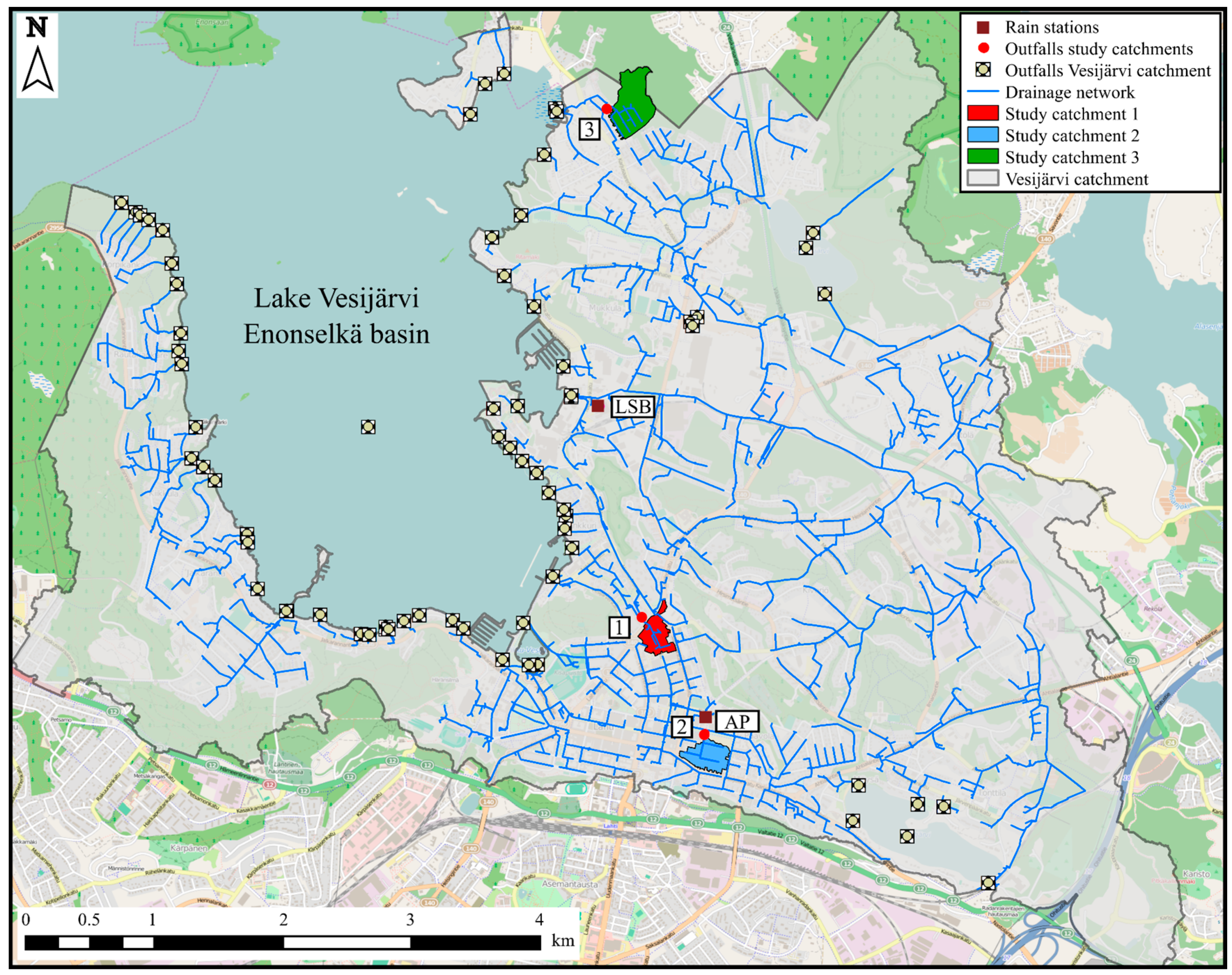
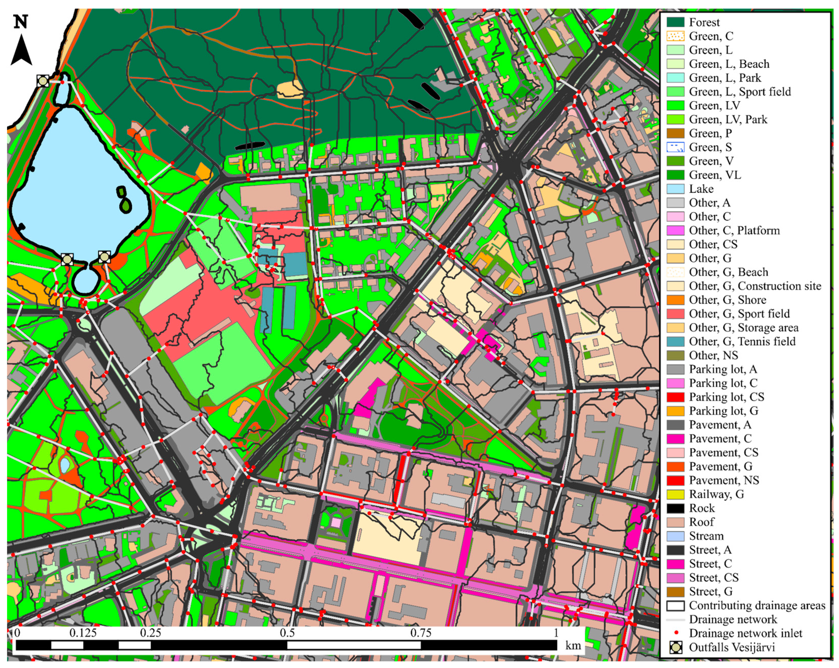
2.1. Study Site and Data

The three study catchments are located within the city of Lahti, southern Finland (Figure 1). The catchments are characterized by varying degrees of impervious cover and land-use intensity, ranging from dense urban land-use in Catchment 1 to suburban residential housing in Catchment 3. The Stormwater Management Model (SWMM) [16,17] was selected as the modeling platform for this study and rainfall–runoff data collected by the University of Helsinki [52,53] between 2008 and 2010 were used for the parameterization of each catchment. Detailed results and further description of the catchments and the hydro-meteorological data are presented in Krebs et al. [23,54] and Valtanen et al. [52,53]. The hydrological impact of perturbations in the resolution of spatial discretization of the urban landscape and infrastructure were explored in Krebs et al. [23]. In the current paper we use the same catchments and data to further investigate the applicability of parameter values calibrated to HR catchments to larger ungauged urban areas and the impact of automated methods for catchment delineation on the simulated runoff.

The Vesijärvi catchment is in this study defined as the area of the city of Lahti that drains into the Enonselkä basin of Lake Vesijärvi (Figure 1). The catchment was selected as the region of interest for upscaling the model results for several reasons: (i) all three study catchments are located within the Vesijärvi catchment; (ii) the catchment covers a large part of the city of Lahti, and is therefore of interest for urban planning; (iii) the water quality of lake Vesijärvi is of substantial interest to the city of Lahti; and (iv) the catchment is ungauged and sufficiently large (30 km²) to pose those challenges that need to be overcome in hydrological assessments of large urban areas. The impervious cover of the Vesijärvi catchment is ca. 27%, of which 25% (6.8% of the whole catchment) consists of roof tops and the remaining 75% (20.5%) is associated with traffic infrastructure, including streets, parking facilities, and sidewalks. The majority of the pervious land-cover consists of natural forested areas (37% of the whole catchment) and cultivated green areas such as yards and parks (12.5% of the catchment). Details on the land-cover of the Vesijärvi catchment and the three study catchments are given in

Table 1. Surface and land-use types and their fractions of the catchment for HR and LR-DEM models of the study catchments 1, 2, and 3, and for the Vesijärvi catchment.

Surface Type	Surface Type CODE	Land-Use Type	1				2				3				Vesijärvi
			Area (ha)		Fraction (%)		Area (ha)		Fraction (%)		Area (ha)		Fraction (%)		Area (ha)	Fraction (%)
			HR	LR DEM	HR	LR DEM	HR	LR DEM	HR	LR DEM	HR	LR DEM	HR	LR DEM
Asphalt	A	Other	-	-	-	-	-	-	-	-	-	0.002	-	0.0	36.2	1.2
		Parking lot	1.505	1.016	25.6	18.7	0.783	0.888	11.8	13.1	0.140	0.163	1.1	1.4	165.3	5.5
		Pavement	0.846	1.048	14.4	19.3	0.412	0.493	6.2	7.3	0.053	0.064	0.4	0.6	83.9	2.8
		Street	1.126	1.075	19.2	19.8	0.492	0.516	7.4	7.6	0.679	0.673	5.4	6.0	157.4	5.3
Concrete	C	Other	-	0.107	-	2.0	-	0.007	-	0.1	-	-	-	-	7.7	0.3
		Parking lot	-	0.044	-	0.8	-	0.051	-	0.8	-	-	-	-	0.7	0.0
		Pavement	-	-	-	-	-	0.114	-	1.7	-	-	-	-	3.9	0.1
		Street	-	-	-	-	-	0.030	-	0.4	-	-	-	-	0.3	0.0
Gravel	G	Other	0.130	0.143	2.2	2.6	0.184	0.023	2.8	0.3	-	-	-	-	72.2	2.4
		Parking lot	0.130	0.002	2.2	0.0	0.892	0.640	13.4	9.5	0.033	0.053	0.3	0.5	23.4	0.8
		Pavement	-	0.004	-	0.1	0.002	0.049	0.0	0.7	0.010	-	0.1	-	37.8	1.3
		Railway	-	-	-	-	-	-	-	-	-	-	-	-	7.4	0.2
		Street	-	-	-	-	0.011	0.011	0.2	0.2	-	-	-	-	7.1	0.2
Natural stone paver	NS	Other	-	-	-	-	-	0.001	-	0.0	-	-	-	-	0.0	0.0
		Pavement	-	-	-	-	-	-	-	-	-	-	-	-	0.0	0.0
Cobble stone	CS	Other	0.247	0.007	4.2	0.1	0.109	0.128	1.6	1.9	0.015	-	0.1	-	3.6	0.1
		Parking lot	-	-	-	-	0.232	0.124	3.5	1.8	0.095	0.006	0.8	0.1	1.4	0.0
		Pavement	-	0.021	-	0.4	0.131	0.017	2.0	0.2	-	-	-	-	0.3	0.0
		Street	-	-	-	-	0.024	-	0.4	-	-	-	-	-	2.3	0.1
Metal sheeting	MS	Roof	1.149	1.474	19.6	27.2	1.275	1.406	19.2	20.8	-	0.915	-	8.1	203.0	6.8
Sheeting			-		-		-		-		0.020		0.2
Tiles/Sheeting	TS		-		-		-		-		1.342		10.7
Crop	CR	Green	-	-	-	-	-	-	-	-	-	-	-	-	33.3	1.1
Lawn	L		0.383	0.099	6.5	1.8	0.325	0.005	4.9	0.1	0.500	0.015	4.0	0.1	75.2	2.5
Lawn/Vegetation	LV		-	0.105	-	1.9	0.493	0.285	7.4	4.2	0.923	2.619	7.3	23.2	262.9	8.8
Peat	P		-	-	-	-	-	-	-	-	-	-	-	-	3.0	0.1
Vegetation/Lawn	VL		-	0.040	-	0.7	0.570	1.503	8.6	22.2	1.198	0.352	9.5	3.1	372.9	12.5
Vegetation	V		0.358	0.241	6.1	4.4	0.697	0.467	10.5	6.9	0.200	0.028	1.6	0.3	234.1	7.9
Swamp	SW		-	-	-	-	-	-	-	-	-	-	-	-	13.2	0.4
Rock	R	Rock	-	-	-	-	-	-	-	-	-	0.266	-	2.4	64.4	2.2
Forest	F	Forest	-	-	-	-	-	-	-	-	7.381	6.137	58.6	54.3	1107.6	37.2
Σ			5.874	5.427	100	100	6.632	6.756	100	100	12.588	11.292	100	100	2980.6	100

. The Vesijärvi catchment is drained through a separate stormwater sewer system and two open streams flowing through the city and draining into Lake Vesijärvi. The stormwater sewer network used for model development considered conduits with a minimum diameter of 300 mm. Krebs et al. [23] proposed this diameter threshold for assessing small-scale processes in large urban areas as it allows: (i) a sufficiently accurate replication of the dynamics of urban runoff and (ii) a feasible model development considering the quality of available spatial data for large areas, where manual correction and complementation of the data is too laborious. The stormwater sewer network in the Vesijärvi catchment has a length of 115.8 km and the open stream length is 28.6 km (

Table 2. Drainage network subdivision for the HR and LR-DEM models of the study catchments and the Vesijärvi catchment.

Drainage Type	Material	1 Length (m)		2 Length (m)		3 Length (m)		Vesijärvi Length (m)
		HR	LR-DEM	HR	LR-DEM	HR	LR-DEM
Conduit	Concrete	762	611	835	624	1649	1041	101,805
	PVC	1851	26	2397	-	-	-	13,957
Open channel	Natural	-	-	-	-	74	-	28,620
∑		2613	637	3232	624	1723	1041	144,382

).

Rainfall input data for simulations of the Vesijärvi catchment were derived from a tipping bucket gauge at Catchment 2 (AP in Figure 1) with a recording interval of 1 minute. Data from this rainfall gauge were already used for calibration and validation of the study catchments [23]. Additionally, rainfall data recorded at 10-min intervals on the roof of the Lahti Science and Business Park (LSB in Figure 1) were available and used for additional validation of the HR study catchment models (VAL-LSB) [23]. Runoff data were recorded at the outfall of each study catchment through 2008–2010 with a 1-min recording interval. The rainfall–runoff data were scanned to identify events where both the rainfall and runoff measurements were functioning [23]. The sequence of events used for calibration (CAL) consists of six, six, and three events for Catchments 1, 2, and 3, respectively. The sequence of validation events using AP rainfall data (VAL-AP) consists of six, five, and one event(s) for Catchments 1, 2, and 3, respectively. The sequence using LSB rainfall data (VAL-LSB) consists of five, three, and eight events for Catchments 1, 2, and 3, respectively. A comprehensive list of rainfall events is given in Krebs et al. [23]. These data are used in this paper to evaluate the impact of DEM-based delineation and model regionalization on simulation results. Spatial data for the discretization of the urban landscape and the drainage network included a DEM (2-m resolution, provided by the Geological Survey of Finland), data on the building roofs and the road network, and digitized maps of the drainage network.

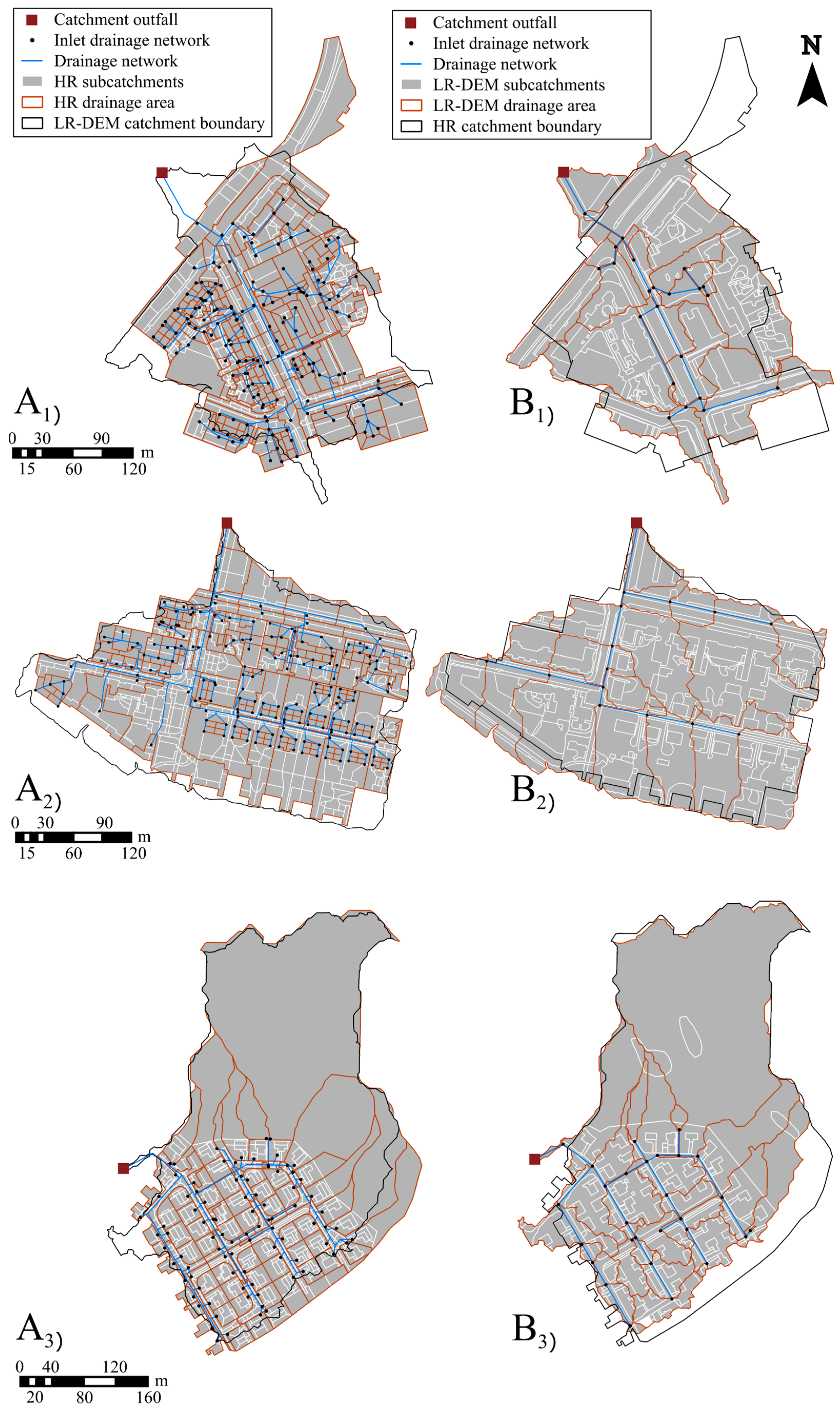
2.2. DEM-Based Delineation (LR-DEM)

Krebs et al. [23] studied the impact of spatial resolution for urban hydrological modeling and concluded that the temporal dynamics can be sufficiently well replicated with a model that (i) discards stormwater sewer conduits with a diameter smaller than 300 mm and (ii) discards surface flow routing between subcatchments before surface runoff enters the drainage network. Reduction of network conduits represented in the model (d_min ≥ 300 mm) results in a replacement of conduit flow by overland flow in the discretized catchment. Additionally, the neglecting of surface flow routing affects the effective impervious area (EIA) [23]. Thus, the approach presented in Krebs et al. [23] implies that EIA equals the total impervious area (TIA) of the catchment. The increase of EIA depends on the catchment structure; the changes were reported to be minor for highly urbanized catchments (+0.3% in Catchment 1) and larger (up to 155% for Catchment 3) for suburban catchments, where impervious surfaces are sometimes not connected to the drainage network [23]. Despite the network conduit and surface flow assumptions, the concept presented by Krebs et al. [23] allows the direct application of LID tools in the model as subcatchment delineation is based on identifying homogeneous surface types (such as rooftops or street sections) at a high spatial resolution.

The LR-DEM model developed in the current study follows the principles described above to maintain the ability to replicate the temporal dynamics of urban runoff. However, the contributing drainage area for each stormwater network inlet is delineated in an automated manner using a DEM (2 m resolution) rather than manually determining the surface routing pattern as in Krebs et al. [23]. While this automated method for catchment delineation is suitable for large urban areas where on-site observation of surface flow patterns is not feasible, small-scale features of the urban landscape (such as street curbs) that are not well presented in DEMs [39,40] will be neglected in the model surface discretization. As a result, the HR and LR-DEM models differ not only in EIA, length of the drainage network, and representation of inter-subcatchment surface flow, but also in terms of catchment boundaries (i.e., area) and consequently the catchment TIA. While this approach obviously discards important information on the catchment, the suggested simplifications for model development allow the assessment of larger urban areas in a feasible manner. Subsurface drainage conduits are naturally not represented in a DEM and, thus, the DEM is commonly pre-processed by burning the conduit network into the DEM surface [22]. In this study a constant value was reduced from DEM grid cells where conduits were located and thereafter depressions filled to allow for hydraulic connectivity. Gironás et al. [22] suggested that all conduits, even though not explicitly modeled, should be included when pre-processing a DEM to allow for realistic drainage basin delineation in urban areas. Following this suggestion, all available conduit information was used to derive the pre-processed DEM, even though only conduits with a minimum diameter of 300 mm were included in the LR-DEM model.

The LR-DEM model was developed using the following steps: (i) the surface was digitized based on both surface (such as asphalt, gravel, or different vegetation types) and land-use types (such as streets, parking lots, or rooftops) derived from spatial data and aerial images (see Table 1); (ii) the stormwater drainage network was digitized using conduits with a minimum diameter of 300 mm; (iii) the contributing drainage area of each inlet present in the minimum diameter was delineated based on the pre-processed DEM; and (iv) the digitized surface map was discretized using the delineated drainage areas resulting in a number of subcatchments per drainage inlet. The described LR-DEM model was developed for the entire Vesijärvi catchment, including the three study catchments.

Krebs et al. [23] concluded that the neglecting of inter-subcatchment surface flow routing for models with lower resolution resulted in decreased model performance for the least urbanized Catchment 3, due to the fact that roof runoff in this catchment is, unlike described in guidelines by the city [55], not drained into the drainage network but onto adjacent green areas. The associated large change in hydraulically connected impervious area when neglecting inter-subcatchment flow resulted in over-prediction of runoff volumes and peaks. Thus, also for the LR-DEM model in this paper, roof runoff was diverted to adjacent green areas in this study catchment. However, this exemption applies only to roof runoff and also in Catchment 3 runoff from all other subcatchments was directly routed to the corresponding drainage network inlet. Surface and conduit related parameters were adopted from the calibrated study catchment model. Model parameters related to the subcatchment and conduit geometry were derived from spatial data. While the subcatchment flow width FW_HR for the HR models was determined using Equation (1), the corresponding flow width FW_LR for the LR-DEM model was determined using Equation (2):

$$F{W}_{HR}=\frac{A}{L}$$

(1)

$$F{W}_{LR}=k\sqrt{A},$$

(2)

where A (m²) is the subcatchment area, L (m) is the length of the overland flow path, and k (-) is a dimensionless coefficient. Krebs et al. [23] determined 0.7 to be a suitable value for k. This value was based on the distribution of k for 2652 subcatchments, for which FW_HR was calculated using Equation (1) and used herein to define FW_LR.

The impact of this automated model parameterization procedure that neglects details of the stormwater drainage description with respect to both the network and surface flow was first evaluated against monitored runoff in the three study catchment. The model performance was thereafter evaluated against the HR model results reported in Krebs et al. [23,54]. The HR study catchment models were used as reference, as they include all catchment details concerning both the surface and network drainage. The model evaluation was conducted both by visual inspection of simulated and observed hydrographs and using model performance statistics. The performance statistics were the Nash-Sutcliffe efficiency E [56], the peak flow error PFE, and the volume error VE.

2.3. Parameter Regionalization

Krebs et al. [23,54] initially developed the HR models for the three study catchments with the aim to assess the much larger ungauged Vesijärvi catchment. The use of separate surface types for catchment subdivision produces a mosaic of subcatchments with homogenous hydrological properties. To allow for the transfer of parameters from sample catchments to an ungauged area, subcatchments with similar homogenous properties (such as a stretch of asphalt street) have to be identified both in each study catchment and in the entire Vesijärvi catchment. In other words, a similar detailed subdivision of the catchment surface for all study catchments and the targeted up-scale area are a prerequisite for the regionalization approach conducted in this study. While this condition mainly concerns the technical applicability of parameter values in the ungauged area, the question remains whether the application is hydrologically justified. The calibration of the HR study catchment models was conducted independently for each catchment [23,54]. Krebs et al. [23] showed that the parameter values calibrated for the same surface types (e.g., an asphalt surface) were similar for each of the three study catchments.

To further investigate the hydrological applicability, in this paper, the parameter sets of each study catchment were applied to the remaining two study catchments to evaluate the regionalization impact on simulated flow. The HR study catchment models were used for this purpose and three parameter sets were defined based on the parameter values calibrated to the study catchments (V₁ for Catchment 1, V₂ for Catchment 2, and V₃ for Catchment 3). Additionally, a reference parameter set (V_Ref) was compiled based on parameter value suggestions given in SWMM user manuals [16,17]. Parameter values were either adopted as the mean value in the case of a suggested parameter value range or as a single suggested value. The application of V_Ref represents a common strategy for the parameterization of ungauged catchments [57] and is thus used herein to evaluate the performance of calibrated parameter values transferred to an ungauged catchment.

For surface types that were not present in the study catchment used for defining the parameter values, the corresponding values were selected from one of the remaining study catchments to attain a complete set of parameters for simulation. Parameters that are specific to a subcatchment rather than a surface type were derived directly from spatial data. Surface-type specific parameters were the depression storage D, Manning’s roughness n_o for overland flow, and the imperviousness I, while the subcatchment slope, the flow width FW_HR or FW_LR, and the subcatchment area depend on the subcatchment geometry. The required model parameter values for the drainage network were derived in a similar manner. However, only the Manning’s roughness n_c for conduit flow is specific for a certain conduit material, while parameters such as the conduit length and slope are specific for each conduit. A full list of values for the three derived parameter sets (V₁, V₂, and V₃) and the reference parameter set V_Ref are given in

Table 3. The parameter sets V₁, V₂, V₃, and V_Ref for the depression storage D, the Manning’s roughness for overland flow n_o, and the imperviousness I. Parameters that were calibrated for the catchment have a gray background, uncalibrated values have a white background, and the subscripts 1–3 indicate from which study catchment values were adopted if corresponding surfaces were missing. Parameter values of V_Ref with subscript a were derived from Rossman [17], values with subscript b were derived from Huber and Dickinson [16], and values with subscript ab were interpolated between suggestions in Rossman [17] and Huber and Dickinson [16]. A description of the “surface type codes” is given in Table 1.

Surface Type	D (mm)				no (−)				I (%)
	V1	V2	V3	VRef	V1	V2	V3	VRef	V1	V2	V3	VRef
A	0.39	0.42	0.62	1.91a	0.011	0.011	0.013	0.007b	100.0	88.5	100.0	100.0
C	0.39	0.42	0.62	1.91a	0.011	0.011	0.013	0.007b	100.0	88.5	100.0	100.0
G	2.54	2.49	2.54	1.91a	0.020	0.030	0.024	0.021b	0–50	33.4	69.5	0
NS	1.01	0.39	1.09	1.91a	0.012	0.020	0.020	0.024a	91	86.6	100.0	100.0
CS	1.01	0.39	1.09	1.91a	0.012	0.020	0.020	0.024a	91	86.6	100.0	100.0
MS	0.18	0.10	2.54	1.91a	0.012	0.011	0.014	0.007ab	100.0	100.0	100.0	100.0
S
TS
CR	4.18	4.13	7.53	7.62a	0.300	0.667	0.790	0.600a	0.0	0.0	0.0	0.0
L	4.98	4.82	5.07	3.81a	0.150	0.168	0.200	0.150b	0.0	0.0	0.0	0.0
LV	4.222	4.22	5.07	5.08a	0.2382	0.238	0.300	0.375ab	0.0	0.0	0.0	0.0
P	7.393	7.393	7.39	7.62a	0.6683	0.6683	0.668	0.600a	0.0	0.0	0.0	0.0
VL	3.592	3.59	2.54	5.08a	0.3262	0.326	0.399	0.375a	0.0	0.0	0.0	0.0
V	4.18	4.13	7.53	7.62a	0.300	0.667	0.790	0.600a	0.0	0.0	0.0	0.0
SW	50.00	50.00	50.00	50.00	0.500	0.500	0.500	0.500	0.0	0.0	0.0	0.0
R	7.393	7.393	7.39	7.62a	0.6683	0.6683	0.668	0.600a	100.0	100.0	100.0	100.0
F	7.393	7.393	7.39	7.62a	0.6683	0.6683	0.668	0.600a	0.0	0.0	0.0	0.0

(surface parameters) and

Table 4. The parameter sets V₁, V₂, V₃, and V_Ref for the Manning’s roughness for conduit flow n_c. Calibrated parameter values have a grey background, un-calibrated values have a white background and the subscripts 1–3 indicate from which study catchment values were adopted if corresponding surfaces were missing. Parameter values of V_Ref were derived from Rossman [17].

Drainage Type	Material	nc (−)
		V1	V2	V3	VRef
Conduit	Concrete	0.011	0.015	0.015	0.013
	PVC	0.011	0.011	0.0112	0.013
Open channel	Natural	0.0493	0.0493	0.049	0.05

(drainage network parameters). The effect of parameter transfer on simulated flow for the HR models was evaluated for the calibration and validation sequences used in Krebs et al. [23] as well as for individual events. Additionally, the hydrological applicability of calibrated parameters to other urban catchments was investigated by applying the three calibrated parameter sets (V₁, V₂, and V₃) and the reference parameter set (V_Ref) to the LR-DEM model to evaluate the parameter set related variation of simulated flow for both the study catchments and the entire Vesijärvi catchment. Details on the hydro-meteorological properties of selected rainfall–runoff events and sequences can be found in Krebs et al. [23].

3. Results

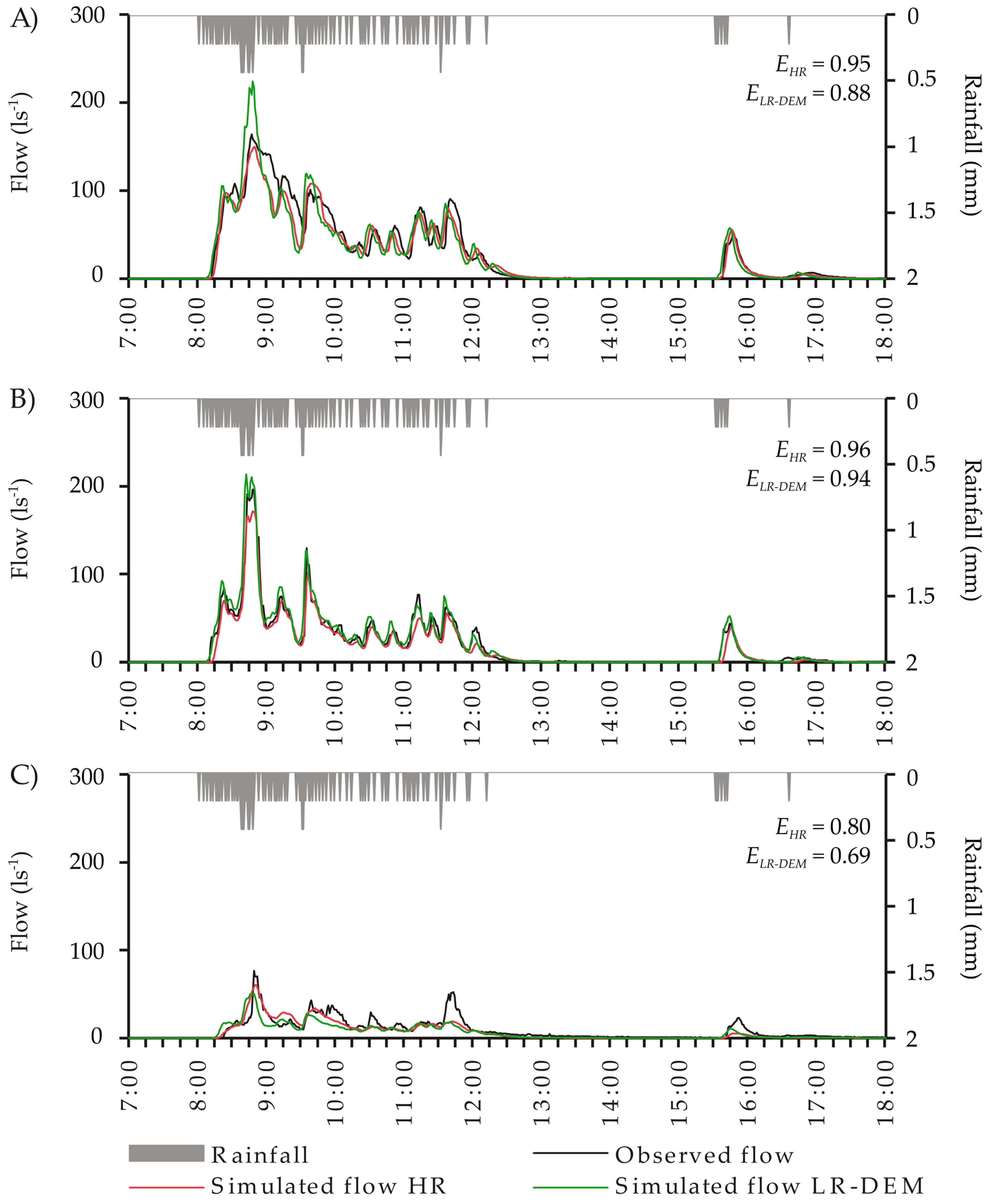
3.1. DEM Delineation

As a result of the DEM delineation, the areas of Catchments 1 and 3 decreased, while the area of Catchment 2 increased compared to the areas determined for the HR models (

Table 5. Catchment properties of the HR and LR-DEM models of the three study catchments and the overlapping and excessive surface areas.

	Unit	1		2		3
		HR	LR-DEM	HR	LR-DEM	HR	LR-DEM
Area	(ha)	5.87	5.43	6.63	6.76	12.59	11.58
TIA	(ha)	5.04	4.79	3.56	3.74	2.37	2.13
EIA	(ha)	5.03	4.79	3.23	3.74	0.93	1.23
Overlapping surface	(%)	100	80	100	97	100	89
Excessive surface	(%)	0	13	0	5	0	3
Subcatchments	(−)	690	317	784	426	821	413
Drainage basins	(−)	160	22	188	15	90	28
Drainage network	(m)	2613	637	3232	628	1722	1041

, Figure 2). While the change of area was similar for the Catchments 1 and 3 (8%) it was smaller for Catchment 2 (2%). The ability of the LR-DEM approach to correctly represent the HR catchments was further evaluated by determination of the overlapping and excessive surface. The first is defined as the fraction of the HR catchment that is included in the LR-DEM catchment and the second defines the fraction of the LR-DEM catchment that is not included in the HR catchment. The best overlap was found for Catchment 2, where 97% of the HR catchment was included in the LR-DEM catchment (i.e., 3% of the HR Catchment 2 were omitted due to the simplification implied by the automated delineation process). For the same catchment, 5% of the LR-DEM catchment surface was excessive; this area was included in the LR-DEM Catchment 2 due to the simplified delineation process. For Catchments 3 and 1 the overlap was lower at 89% and 80%, respectively, and while the excessive surface for Catchment 3 was 3% it was clearly higher (13%) for Catchment 1 (Table 5). As runoff generation in urban areas is dominated by processes on impervious surfaces, the simulated runoff volume and dynamics are not only affected by the change in catchment size, but also by the associated alteration in both TIA and EIA. The HR model of Catchment 1 had a TIA of 5.04 ha, of which most of the area was hydraulically effective (EIA 5.03 ha), while both the EIA and TIA of the LR-DEM model were lower at 4.79 ha. The fraction of hydraulically connected impervious surfaces was smaller for the HR model of Catchment 2, for which EIA and TIA were 3.23 ha and 3.56 ha, respectively. Besides the catchment area, also EIA increases for the LR-DEM model of Catchment 2 to 3.74 ha as most of the excessive catchment area comprised rooftops and street sections. For Catchment 3, the reduction in TIA is proportional to the reduction of catchment area and TIA reduces from 2.37 ha (HR model) to 2.13 ha (LR-DEM model). However, as stated above, EIA does not equal TIA for this catchment due to roof runoff routing onto adjacent green areas. The neglecting of inter-subcatchment surface flow routing in the LR-DEM model, while maintaining the original surface flow pattern for roofs (onto adjacent green areas) results in EIA of 1.23 ha consisting of streets, pavements and driveways. This corresponds to an increase of 0.3 ha (32%) in EIA compared to the HR model of Catchment 3. Roofs account for 0.9 ha in Catchment 3 and also remain hydraulically disconnected from the network in the LR-DEM model setup. The boundaries, contributing drainage areas for each inlet, and subcatchments of the three study catchments are illustrated in Figure 2.

Differences in catchment area, TIA, and EIA naturally affect the simulated catchment runoff (Figure 3,

Table 6. Model performance statistics (efficiency E, absolute peak flow error ABS PFE, and volume error VE) for the HR and LR-DEM models of the study Catchments 1, 2, and 3 for the alternative parameter sets V₁, V₂, V₃, and V_Ref and the three studied sequences of events. Performance statistics with a grey background were produced by the parameter set specifically calibrated to the study catchment. ABS PFE in the first row of each parameter set represents the mean value for the sequence events while the values given in parentheses represent the range of ABS PFE.

Sequence	Resolution	Parameter Set	E (−)			ABS PFE (%)			VE (%)
			1	2	3	1	2	3	1	2	3
CAL	HR	V1	0.88	0.93	0.71	12.4	17.1	29.2	7.0	−1.8	26.8
						(4.1–20.4)	(4.0–37.3)	(6.4–51.5)
		V2	0.86	0.97	0.73	21.3	13.1	35.4	18.7	9.3	36.1
						(10.3–33.8)	(3.3–24.9)	(4.4–56.5)
		V3	0.81	0.91	0.80	24.6	25.8	35.7	14.6	4.0	32.2
						(2.5–53.9)	(0.7–53.1)	(20.9–53.3)
		VRef	0.73	0.89	0.75	30.7	34.3	42.6	25.6	22.5	36.8
						(2.1–99.8)	(3.4–100.0)	(17.2–79.2)
	LR-DEM	V1	0.87	0.58	0.66	23.9	53.9	25.7	6.5	−29.2	31.4
						(5.9–86.7)	(19.2–77.8)	(7.9–36.3)
		V2	0.91	0.82	0.66	14.4	31.2	33.2	15.1	−19.5	38.3
						(0.3–22.6)	(5.2–51.3)	(18.7–41.5)
		V3	0.87	0.74	0.70	23.5	37.9	26.5	18.1	−18.4	32.2
						(2.2–54.6)	(24.0–49.4)	(9.0–36.3)
		VRef	0.74	0.65	0.66	38.1	53.1	45.5	26.9	1.8	38.6
						(6.5–100.0)	(26.2–100.0)	(35.3–65.9)
VAL-AP	HR	V1	0.85	0.93	0.64	8.1	10.5	3.8	6.5	8.9	5.0
						(0.0–27.6)	(1.1–30.1)	-
		V2	0.83	0.94	0.67	17.8	16.1	16.7	18.2	17.8	13.7
						(12.3–27.5)	(7.0–38.4)
		V3	0.81	0.91	0.66	26.6	22.6	29.0	13.3	12.7	16.1
						(11.8–42.0)	(1.7–43.0)	-
		VRef	0.81	0.84	0.64	21.9	24.9	27.1	21.0	29.5	23.3
						(4.7–46.5)	(9.6–39.2)	-
	LR-DEM	V1	0.81	0.79	0.40	26.0	37.3	12.2	4.5	−12.3	26.1
						(7.2–65.8)	(11.2–64.4)	-
		V2	0.86	0.90	0.54	10.6	18.5	8.6	14.5	−1.0	34.2
						(4.2–22.7)	(2.8–40.1)	-
		V3	0.85	0.92	0.56	19.3	12.9	2.1	14.2	−1.6	27.9
						(0.4–44.7)	(2.6–21.1)	-
		VRef	0.76	0.85	0.52	26.6	12.6	0.3	20.2	12.5	37.5
						(4.6–49.4)	(1.7–22.2)	-
VAL-LSB	HR	V1	0.84	0.59	0.78	13.7	16.2	26.3	3.7	−1.0	11.4
						(0.3–26.5)	(4.7–23.3)	(1.2–69.4)
		V2	0.82	0.61	0.80	30.1	21.9	37.0	16.3	9.7	24.0
						(18.7–38.0)	(2.9–34.6)	(2.7–75.2)
		V3	0.80	0.54	0.81	26.8	15.8	33.8	11.4	0.5	19.9
						(18.0–36.1)	(5.7–23.2)	(2.6–71.4)
		VRef	0.78	0.60	0.78	20.6	21.4	33.0	18.3	17.1	31.5
						(7.8–34.0)	(6.7–28.9)	(0.1–70.9)
	LR-DEM	V1	0.83	0.45	0.65	25.3	8.3	33.0	1.4	−24.6	16.4
						(0.6–46.9)	(0.2–20.6)	(11.1–96.4)
		V2	0.87	0.53	0.72	17.1	12.8	35.4	10.8	−14.9	25.4
						(2.5–32.2)	(11.5–13.8)	(10.5–67.3)
		V3	0.86	0.43	0.75	15.9	7.9	27.6	10.8	−19.9	19.0
						(2.9–35.8)	(1.0–21.2)	(1.8–64.4)
		VRef	0.79	0.49	0.73	22.6	10.9	28.3	16.7	−3.4	33.8
						(4.6–32.4)	(6.1–15.0)	(0.9–64.2)

). The effects were evaluated by comparison of LR-DEM simulated runoff for Catchments 1, 2, and 3 with HR simulated and observed runoff through visual hydrograph inspection and evaluation of model performance statistics. The smallest impact of DEM delineation on simulated runoff was found for Catchment 1, for which the LR-DEM model yielded a similar efficiency E (0.87) for the calibration sequence (CAL) than achieved with the HR model (0.88). A similar minor degradation in efficiency was found for the LSB validation sequence where the LR-DEM model achieved an efficiency of 0.83 compared to 0.84 achieved by the HR model. The degradation in model efficiency for VAL-AP was slightly larger with an efficiency of 0.81 for the LR-DEM model compared to 0.85 achieved by the HR model. In terms of simulated runoff volumes only small impacts were observed with the LR-DEM and HR model producing similar volume errors VE (3.7%–7.0% for the HR model compared to 1.4%–6.5% for the LR DEM model) for the three simulation sequences of Catchment 1. The largest impact of the lower resolution and the DEM delineation method on model performance for Catchment 1 can be seen in the peak flow errors (PFE). While the HR model absolute mean PFE for simulated events was 12.4%, 8.1%, and 13.7%, for CAL, VAL-AP, and VAL-LSB, respectively, it increased to 23.9%, 26.0%, and 25.3%, for the same sequences of Catchment 1 using the LR-DEM model.

The LR-DEM model efficiency for Catchment 2 showed a larger decrease from the HR simulations than was found for Catchment 1, especially for CAL. However, the performance remained acceptable for both CAL (E = 0.82) and VAL-AP (E = 0.90) (Table 6). The performance for VAL-LSB was lower (E = 0.53), but it should be noted that for this sequence also the HR model produced lower efficiencies (0.61), which may be explained by the relatively large distance between the LSB rainfall station and Catchment 2. With an increasing distance, the temporal dynamics of recorded rainfall and runoff show lower correspondence, which negatively affects simulation results [23]. The capability of the LR-DEM model to replicate observed peak flows in Catchment 2 was better than for Catchment 1, but it can be noted also here that PFE is the most sensitive performance criterion in terms of accurate surface flow routing. The impact of the lower resolution on the simulated runoff volume is larger for Catchment 2 compared to Catchment 1, but VE remains within acceptable limits (ranging from −1 to 19.5%) for Catchment 2.

The impact of the LR-DEM model development procedure on simulation results for Catchment 3 was comparable to that seen for Catchment 2. The LR-DEM model achieved efficiencies of 0.70 (HR model 0.80), 0.56 (0.66), and 0.75 (0.81), for CAL, VAL-AP, and VAL-LSB, respectively. It is to be noted, however, that for Catchment 3 only a single event was available for VAL-AP, due to the remote location of the catchment related to the rainfall measurement station. The change in PFE was the smallest for all three catchments except for the single AP validation event. In terms of VE, the LR-DEM and HR model performed equally well, with identical or very similar errors for CAL and VAL-LSB. Again, a larger change was found for the AP validation event.

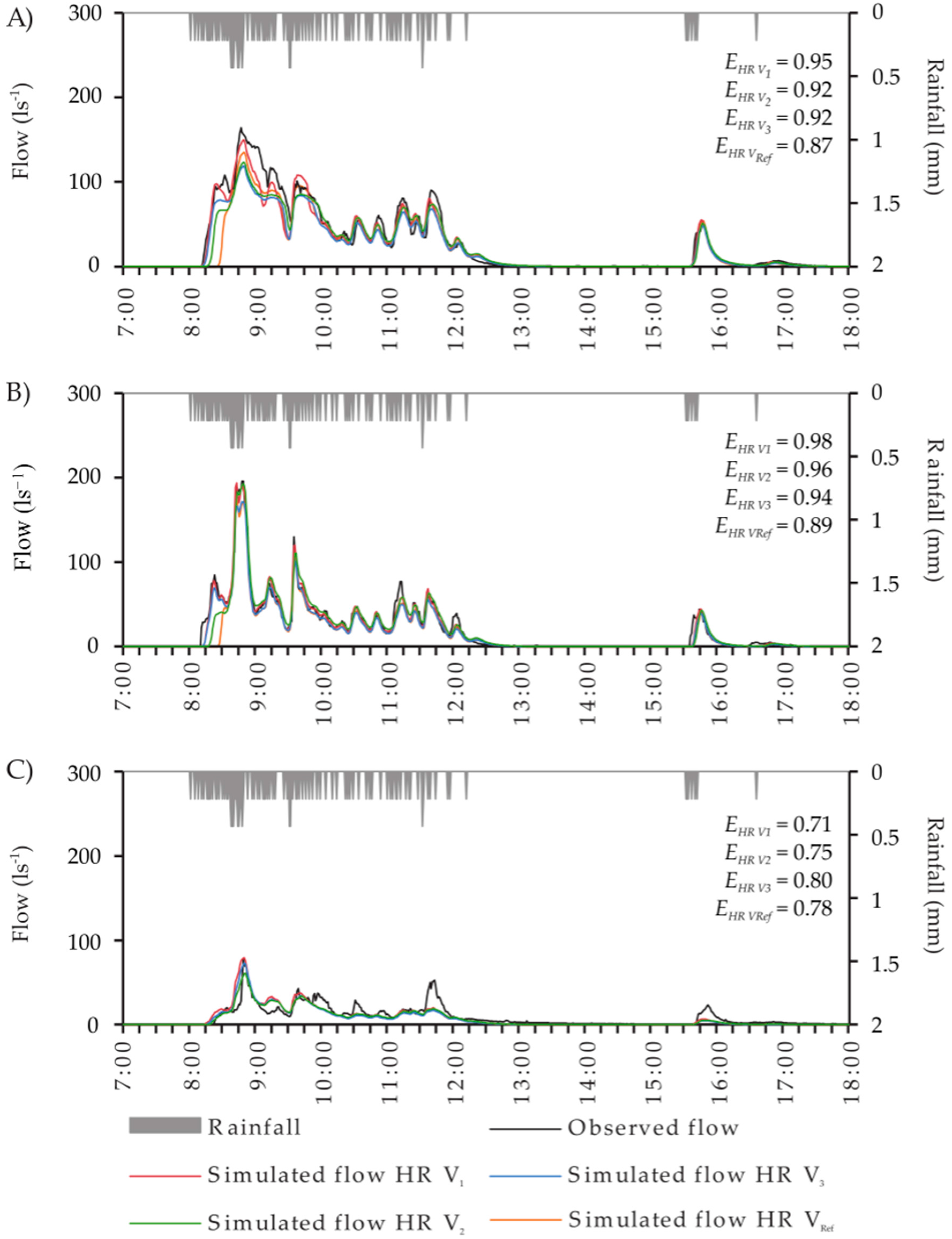
3.2. Parameter Regionalization

Application of model parameters to larger, ungauged areas necessitates that a model parameter set calibrated to one catchment also produces acceptable simulation results for other catchments within the same region. Thus, parameter sets calibrated for the HR models of Catchment 1 (V₁), 2 (V₂), and 3 (V₃) (Table 3 and Table 4) were applied to the other two catchments to evaluate the performance difference to the parameter set specifically calibrated to the catchment. Additionally, the reference parameter set V_Ref was applied to each of the study catchments. As the large-scale Vesijärvi catchment model was developed using the LR-DEM methodology the performance of regionalized parameters (V₁, V₂, V₃, and V_Ref) was furthermore investigated for the LR-DEM models of the three study catchments. The performance of parameter transfer was evaluated using events of the calibration and validation periods for each catchment investigating both the entire sequences and individual events; the impact of parameter transfer was thus evaluated for a total of 18 simulation sequences (HR and LR-DEM models for each catchment using three sequences each, Table 6) and a total of 86 simulation events.

With respect to model efficiency E, the specifically calibrated parameter set achieved the best performance for 13 of the 18 sequences; while for five sequences a transferred parameter set outperformed the specifically calibrated set, V_Ref did not achieve a higher efficiency for any of the evaluated sequences (Table 6). For the simulation events, the specifically calibrated parameter set achieved a mean efficiency E of 0.76. While the transferred parameter sets achieved a mean efficiency E of 0.70, V_Ref yielded a lower mean efficiency of 0.52. The specifically calibrated parameter set achieved the best efficiency for 62% of the events. For 35% of the simulation events a transferred parameter set achieved the highest efficiency, while V_Ref yielded the highest efficiency for 3% of the events. While the efficiency of V_Ref was inferior to both transferred sets for 70% of the simulation events, it outperformed the transferred sets for 9% of the events.

With respect to the simulated runoff volume for entire simulation sequences, a better replication of sequences was achieved by the transferred parameter sets compared to specifically calibrated parameters; while the specific parameter sets produced the most accurate volume replication for seven of the 18 sequences, nine of the sequences were best simulated by a transferred parameter set, and the volume of two sequences was best replicated using V_Ref (Table 6). The best performing parameter set concerning runoff volume was V₁, which performed best for all sequences of Catchment 1 (for which it was calibrated) as well as for all sequences of Catchment 3. It is to be noted, however, that a low VE for a sequence of events may also be achieved even though the VE for individual events is high. This would be the case if there is a balance between events with a volume underestimation and a volume overestimation. When looking at individual simulation events, the specifically calibrated parameter sets produced a lower mean absolute volume error (17.8%) compared to the performance of the transferred sets (21.9%), while V_Ref yielded a clearly larger mean volume error (33.9%). The specifically calibrated parameter set produced the smallest volume errors (VE) for 40% of the simulation events, and while for 49% of the events a transferred parameter set produced the smallest VE, V_Ref performed best for 11% of the simulation events. While V_Ref produced a larger volume error than both transferred sets for 72% of the simulation events, it outperformed the transferred sets for 13% of the events.

The performance of parameter sets concerning the simulated peak flow was similar to the performance found for the runoff volume. For six sequences the best mean PFE was achieved using the specifically calibrated parameter set, for 10 sequences the lowest mean PFE was achieved by a transferred set, and for two sequences V_Ref showed the best performance. For 11 of the 18 sequences, V_Ref produced a higher mean PFE than both transferred parameter sets, while both transferred sets were outperformed by V_Ref for four sequences. Also, the results for simulation events were similar to the ones observed for the runoff volume; for 34% of the simulation events the specifically calibrated parameter set produced the smallest PFE and while the smallest PFE was achieved for the majority of events (56%) using a transferred set, V_Ref achieved the best results for only 10% of the events. However, while concerning E and VE V_Ref was clearly inferior compared to the transferred parameter sets, the results concerning PFE were more vague; while V_Ref was inferior to the transferred sets for 38% of the simulation events, the reference parameter set performed better than both transferred parameter sets for 29% of the simulation events. Also, the difference in mean absolute PFE was smaller than for VE with 21.7% for the specifically calibrated sets compared to 24.6% for the transferred sets and 29.2% achieved by V_Ref. Figure 4 illustrates the observed and HR simulated flow with V₁, V₂, V₃, and V_Ref for an event used for all three catchments and Figure 5 illustrates the observed and LR-DEM simulated flow for all parameter sets for the same event.

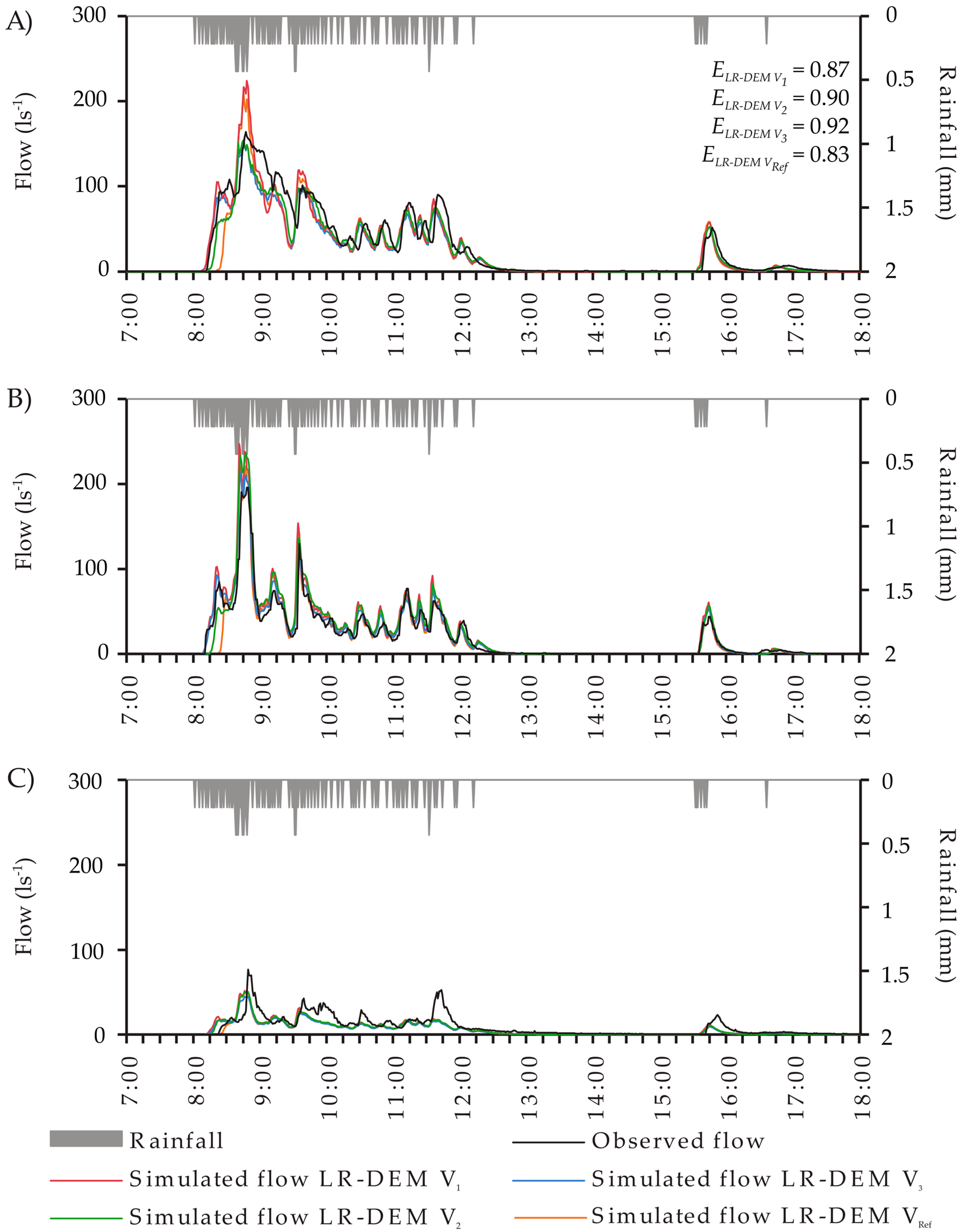
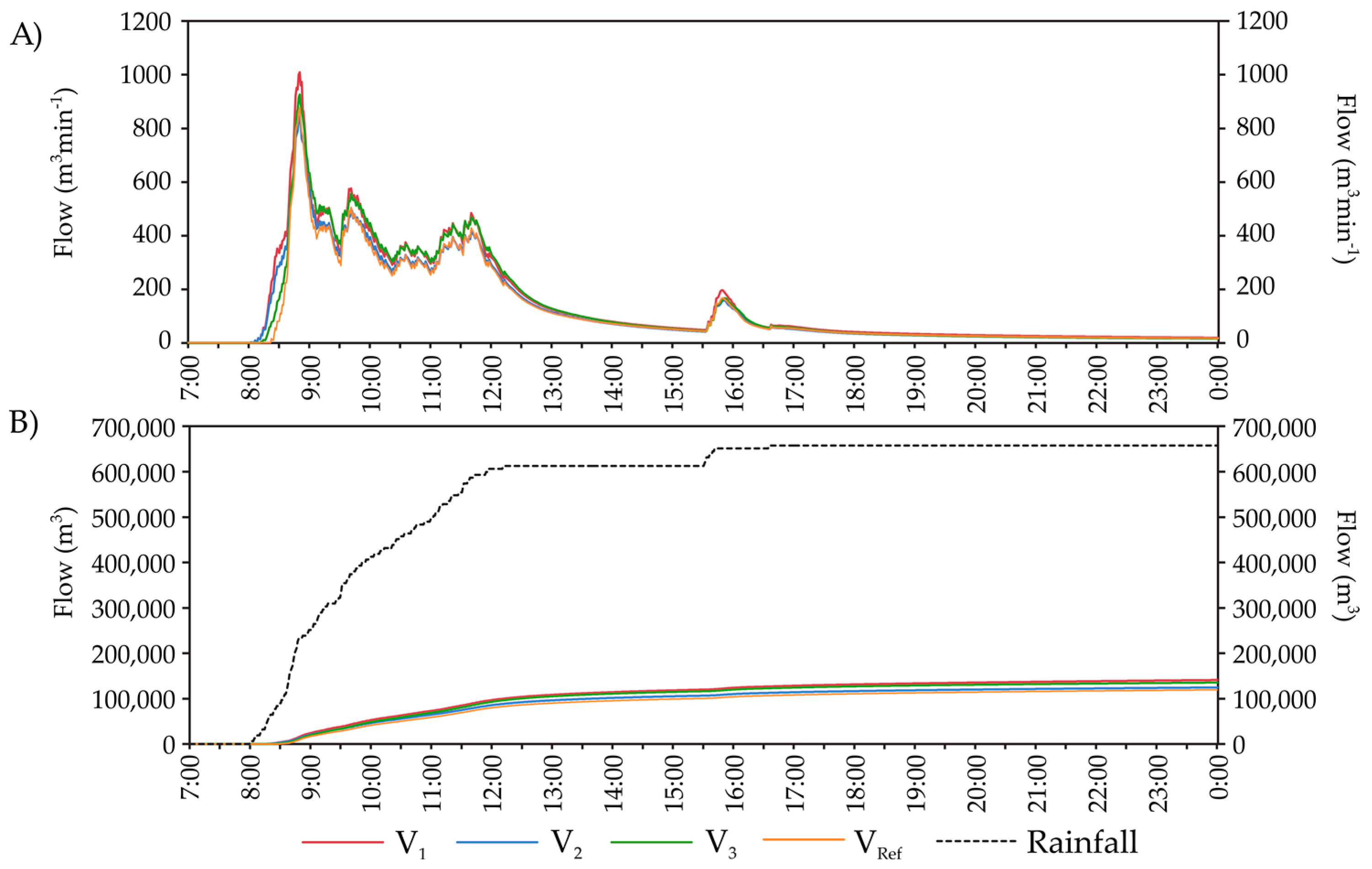
3.3. Vesijärvi Catchment Model

The entire Vesijärvi catchment of the city of Lahti was parameterized using the LR-DEM methodology and the parameter sets V₁, V₂, V₃, and V_Ref. Forested areas account for the largest fraction in the catchment (37.2% or 1108 ha), followed by other green areas (33.4% or 995 ha). The impervious cover of the catchment is 27.3%, consisting of roofs (6.8% of the total catchment area) and traffic-related surfaces (20.5%) such as streets, parking areas, and sidewalks (Table 1). The catchment discretization for the model resulted in a total of 56,037 subcatchments that are drained through a drainage network of 144.4 km. The network comprises of 115.8 km of stormwater sewers, 28.6 km of streams (Table 2), and 5574 inlet nodes. The network drains into Lake Vesijärvi via 71 outfalls that include both sewer conduit and stream outfalls into the lake. A section of the model covering a fraction of the city center is presented in Figure 6 and the total surface runoff received by Lake Vesijärvi for one event is shown in Figure 7.

4. Discussion

In this paper we complemented the methodology presented by Krebs et al. [23] by using a DEM to define contributing drainage areas for drainage network inlets rather than information acquired during on-site visits. This addition extends the applicability of the methodology to considerably larger urban areas than the small monitored catchments. The impact of DEM delineation on model performance was assessed against results of Krebs et al. [23], where catchments were delineated using information gathered during site visits.

No correlation between the degree of urbanization and the error in catchment size was observed. While for the most urbanized Catchment 1 and the least urbanized Catchment 3 the catchment area decreased by 8% and 10%, respectively, the area of the moderately urbanized Catchment 2 increased by 2%. However, the change in EIA that is induced by the negligence of inter-subcatchment surface flow routing correlated with the degree of urbanization, with the smallest impact found for Catchment 1 (−5%), followed by Catchment 2 (15%) and Catchment 3 (30%). It is noteworthy, however, that inter-subcatchment surface flow was maintained for roofs in the LR-DEM model of Catchment 3, in which, contradicting city guidelines [55], roof runoff is not routed into the drainage network but rather to adjacent pervious areas. If roofs had been hydraulically connected in Catchment 3, EIA would have increased by 129%, producing inacceptable simulation results. While not investigated in this study, the large effect of roofs on EIA in Catchment 3 indicates the potential of roof runoff disconnection as a measure for stormwater management.

Jankowfsky et al. [33] studied different automated catchment delineation methods for a 3.5 km² peri-urban catchment in France and compared them with a method where topographical data were complemented with field observations. Their study produced subcatchment area overlaps of 85%–98% depending on the automated method used and the corresponding excessive surface fractions were 1%–15%. It has to be noted, however, that the DEM used for a part of their catchment had a much lower resolution (25 m) compared to the DEM used in our study (2 m). The results produced for the study catchments in our study are in accordance with those presented by Jankowfsky et al. [33], with the lowest errors found for Catchment 2 (97% overlap and 5% excessive surface) and the highest errors found for Catchment 1 (80% overlap and 13% excessive surface). The rather large errors in both overlap and excessive surface for Catchment 1 are due to a street area in the northeast of the catchment, which, considering sewer inlets, is outside the catchment area (see Figure 2A₁,B₁). This stretch of street consists of a rather steep curve with sewer inlets located at the outer edges of the curve. As a result, street runoff actually bypasses the designated inlets connected to a sewer line outside Catchment 1 and drains into Catchment 1 instead. This reveals how the impact of small details on catchment delineation are specific to urban areas but neglected in most automated approaches, as suggested by earlier studies [22,40].

The alteration in catchment properties that is induced by the automated DEM delineation naturally affects the simulated runoff. However, both the Nash–Sutcliffe efficiency E and the volume error VE remained within acceptable limits for all catchments in the current study. The results indicate that the simulated runoff is more affected by the alteration in EIA, induced by the negligence of inter-subcatchment surface flow, rather than the DEM delineation itself. The largest change in VE was found for simulations of Catchment 2, for which also the change in EIA was the largest. For Catchments 1 and 3, the LR-DEM delineation had less effect on the runoff volume, which can be explained by smaller alterations in EIA due to the high degree of urbanization in Catchment 1 (the difference between TIA and EIA is negligible) and the routing of roof runoff in Catchment 3. For all three catchments the peak flow error PFE was most sensitive to the inaccuracies arising from the DEM-based catchment delineation. These results indicate that PFE is more sensitive to accurate catchment delineation and overland flow routing than the volume error and the Nash–Sutcliffe efficiency E. Consequently, the selection of spatial and temporal model resolution and the used accuracy for catchment delineation depend on the objective of the hydrological assessment as accurate simulations of the peak flow require a more precise model description than the simulation of runoff volume or the shape of the runoff hydrograph.

Several studies have addressed the model parameterization of ungauged areas where a direct calibration of model parameters is not possible [41,44,47,50,51]. Seibert [45] used parameter–catchment relationships for model regionalization and reported a large decrease in model efficiency. Merz and Blöschl [47] used various regionalization approaches and came to the conclusion that hydrological catchment differences need to be accounted for and a mean of calibrated parameter values as well as a single “expert judgement” produced poor simulation results. Parajka et al. [51] studied a variety of regionalization methods (such as parameter mean, spatial proximity, regression, and site-similarity) and achieved the best results with a kriging approach and a site-similarity using a donor catchment with similar hydrological properties. Kokkonen et al. [50] suggested that the mean of available calibrated parameter sets is not sufficient to properly parameterize an ungauged catchment; parameters transferred from hydrologically similar catchments produced results that were not much inferior to results achieved by locally calibrated parameter sets. In this paper, we propose a methodology to parameterize large urban catchments by a regionalization of parameters calibrated to data from high-resolution study catchments. The key basis of this approach is a surface discretization that produces subcatchments with homogenous surface properties. The surface discretization was mostly based on spatial data readily available for both the small-scale study catchments and the larger, ungauged Vesijärvi catchment. Compared to earlier work, the proposed methodology can be classified as a site-similarity approach [41,50,51]. However, the site-similarity used in our approach is independent from the actual surface structure (i.e., degree of urbanization) of both the calibrated and ungauged areas and rather created by identifying homogenous urban surface types at a high spatial resolution. This approach allows the definition of parameters that can be assigned to the corresponding surfaces (e.g., a stretch of street or a roof) in the ungauged catchment. Krebs et al. [23] showed a high correlation between parameters independently calibrated to our three study catchments, which supports the applicability to an ungauged area. In this study, three parameter sets (V₁, V₂, and V₃ based on the calibration to the three study catchments) were defined and inter-changed between the study catchments for both the HR and the proposed LR-DEM model setups.

The presented results indicate that while an overall better simulation performance was achieved by the specifically calibrated parameter sets, the performance of transferred parameter sets was not much inferior. Concerning both the shape of the hydrograph and the simulated runoff volume, transferred parameter sets performed better than the compiled reference parameter set V_Ref; transferred sets achieved a mean efficiency E of 0.70 and a mean absolute VE of 21.9% compared to E of 0.52 and VE of 33.9% for V_Ref. While a better performance of transferred sets (PFE of 24.6%) compared to V_Ref (PFE of 29.2%) was also observed for the simulated peak flow, the advantage of calibrated parameters over a parameter set based on literature suggestions was less clear. It is to be noted that while the model efficiency E was used as an objective function during calibration, neither the runoff volume nor the peak flow rate were optimized during calibration. Therefore, while the site-specific parameter sets clearly outperformed the transferred sets with respect to model efficiency, the results concerning the runoff volume and peak flow rate are less clear. Of the evaluated objectives, the peak flow error was found to be the most sensitive evaluation criterion to the transfer of model parameter values. While earlier regionalization studies reported varying success, the surface type-based model regionalization approach produced overall good results. However, none of the earlier studies were explicitly focusing on urban areas. Runoff processes in urban areas are dominated by impervious surfaces whose high fraction together with an efficient drainage system make the rainfall–runoff response more straightforward than in natural catchments. Regionalization of hydrological model parametrizations is likely to be easier in the urban setting, where the runoff response is easier to describe as long as the input rainfall data have sufficiently high temporal resolution and accuracy.

Several studies have shown that a high spatial resolution can improve simulation results and reduce the number of calibration parameters [9,22,54,58]. However, a high spatial resolution can also produce a large number of calibration parameters implying a model over-parameterization. In other words, the impact of an inappropriate parameter value is compensated by an inappropriate value of another parameter, resulting in poor predictive model capability [59] and affecting the model reliability and robustness [60]. While the methodology presented in this paper uses a high spatial resolution, the number of calibration parameters, due to the use of surface type subcatchments with homogeneous hydrological properties, is relatively low (8–25 calibration parameters depending on the catchment) considering the detailed description of the surface and drainage network. Furthermore, the identifiability of parameter values is indicated by (i) similar calibrated parameter values for same surfaces in the three study catchments despite the independent calibration; (ii) good performance of transferred parameter sets in all three catchments despite the differences in catchment characteristics (e.g., imperviousness as well as the composition of the impervious cover); and (iii) good model performance for a large number of rainfall events with varying rainfall depth, intensity, and duration. The same observations also indicate that the model calibrations produced reliable parameter sets. As stated above, two rainfall stations were available for the hydrological assessments in this study. In particular, the distances between Catchment 3 and the AP station (4.9 km) and Catchment 2 and the LSB station (2.7 km) are relatively large. With increasing distance between the measurement stations the recorded rainfall and runoff become less consistent, i.e., the measured rainfall differs from the rainfall that generated the measured runoff. This might lead to a model calibration that compensates for an inadequate rainfall input rather than producing a robust parameter set. However, the stated observations show that the measured rainfall was, despite the partly relatively large distance, sufficiently similar to the rainfall that generated the monitored runoff.

The methodology proposed in this paper to parameterize a large, ungauged, urban area, was applied to the Vesijärvi catchment of the city of Lahti to test the feasibility of the approach. Despite the reduction in the data requirement manual work remained necessary to conceptualize the catchment. However, the work load required remained acceptable considering the size of the catchment (30 km²) and the spatial detail used for the surface description. This detail allows for an explicit spatial description of LID tools also in the city-scale modeling studies. While it is acknowledged that the hydrological evaluation of various LID scenarios requires an explicit and spatially highly distributed modeling approach [19], LID assessments are still commonly simulated by alteration of lumped parameters [25]. Besides for assessments of LID strategies, the proposed methodology is also suited for assessing the hydrological effects of urban land-cover changes, such as urban densification or the construction of new sites. The large Vesijärvi catchment model parameterized in this study allows urban planners and engineers to evaluate potential LID benefits on the city scale, concerning both the optimal placement and the types of LID tools, especially in the light of a given financial budget.

5. Concluding Remarks

Based on the presented results, we conclude that:

• while the simplifications induced by the automated, DEM-based delineation process affect the simulated urban runoff, the simulation results remain acceptable;
• a transfer of parameter values that were calibrated to high-resolution study catchments to ungauged areas is preferable to a parameterization using the available literature;
• simulation results for three different urban catchments and a large number of rainfall events with varying characteristics show that the proposed catchment discretization produces identifiable model parameters; and
• the detailed surface discretization allows for the explicit spatial description of various LID scenarios (e.g., green roofs, pervious pavers, or disconnection of impervious surfaces), supporting the evaluation of alternative urban water management strategies.

References

1. Schueler, T.R. The importance of imperviousness. Watershed Prot. Tech. 1994, 1, 100–111. [Google Scholar]
2. Arnold, C.L., Jr.; Gibbons, C.J. Impervious surface coverage: The emergence of a key environmental indicator. J. Am. Plan. Assoc. 1996, 62, 243–258. [Google Scholar] [CrossRef]
3. Bannerman, R.T.; Owens, D.W.; Dodds, R.B.; Hornewer, N.J. Sources of pollutants in Wisconsin stormwater. Water Sci. Technol. 1993, 28, 241–259. [Google Scholar]
4. Beighley, E.; Kargar, M.; He, Y. Effects of impervious area estimation methods on simulated peak discharges. J. Hydrol. Eng. 2009, 14, 388–398. [Google Scholar] [CrossRef]
5. Booth, D.B.; Jackson, C.R. Urbanization of aquatic systems: Degradation thresholds, stormwater detection, and the limits of mitigation. J. Am. Water Resour. Assoc. 1997, 33, 1077–1090. [Google Scholar] [CrossRef]
6. Brabec, E.A. Imperviousness and land-use policy: Toward an effective approach to watershed planning. J. Hydrol. Eng. 2009, 14, 425–433. [Google Scholar] [CrossRef]
7. Guan, M.; Sillanpää, N.; Koivusalo, H. Modelling and assessment of hydrological changes in a developing urban catchment. Hydrol. Process. 2015, 29, 2880–2894. [Google Scholar] [CrossRef]
8. Haase, D. Effects of urbanisation on the water balance-A long-term trajectory. Environ. Impact Assess. Rev. 2009, 29, 211–219. [Google Scholar] [CrossRef]
9. Lee, J.G.; Heaney, J.P. Estimation of urban imperviousness and its impacts on storm water systems. J. Water Resour. Plan. Manag. 2003, 129, 419–426. [Google Scholar] [CrossRef]
10. Ruth, O. The effects of de-icing in Helsinki urban streams, Southern Finland. Water Sci. Technol. 2003, 48, 33–43. [Google Scholar] [PubMed]
11. Maksimovic, C. General overview of urban drainage principles and practice. In Urban Drainage in Specific Climates, Volume 2: Urban Drainage in Cold Climates; Saegrov, S., Milina, J., Thorolfsson, S., Eds.; UNESCO: Paris, France, 2000; pp. 1–21. [Google Scholar]
12. The United States Environmental Protection Agency (US EPA). Low Impact Development (LID)—A Literature Review; US EPA Office of Water: Washington, DC, USA, 2000.
13. Roy, A.H.; Wenger, S.J.; Fletcher, T.D.; Walsh, C.J.; Ladson, A.R.; Shuster, W.D.; Thurston, H.W.; Brown, R.R. Impediments and solutions to sustainable, watershed-scale urban stormwater management: Lessons from Australia and the United States. Environ. Manag. 2008, 42, 344–359. [Google Scholar] [CrossRef] [PubMed]
14. Butler, D.; Davies, J.W. Urban Drainage, 3rd ed.; Spon Press: Oxon, UK, 2011. [Google Scholar]
15. Cheng, M.-S.; Coffman, L.S.; Clar, M.L. Low-impact development hydrologic analysis. In Proceedings of the Specialty Symposium Held in Conjunction with the World Water and Environmental Resources Congress, Orlando, FL, USA, 20–24 May 2001; Brashear, R.W., Maksimovic, C., Eds.; ASCE: Orlando, FL, USA, 2001; pp. 659–681. [Google Scholar]
16. Huber, W.C.; Dickinson, R.E. Storm Water Management Model Manual Version 4: User’s Manual; US EPA: Athens, GA, USA, 1988.
17. Rossman, L.A. Storm Water Management Model User’s Manual Version 5; US EPA National Risk Management Research Laboratory: Cincinnati, OH, USA, 2010.
18. Elliott, A.H.; Trowsdale, S.A. A review of models for low impact urban stormwater drainage. Environ. Model. Softw. 2007, 22, 394–405. [Google Scholar] [CrossRef]
19. Amaguchi, H.; Kawamura, A.; Olsson, J.; Takasaki, T. Development and testing of a distributed urban storm runoff event model with a vector-based catchment delineation. J. Hydrol. 2012, 420–421, 205–215. [Google Scholar] [CrossRef]
20. Rodriguez, F.; Andrieu, H.; Creutin, J.-D. Surface runoff in urban catchments: morphological identification of unit hydrographs from urban databanks. J. Hydrol. 2003, 283, 146–168. [Google Scholar] [CrossRef]
21. Cantone, J.P.; Schmidt, A.R. An innovative approach for modeling large urban hydrologic systems. In Proceedings of the World Environmental and Water Resources Congress, Kansas City, MO, USA, 17–21 May 2009; ASCE: Reston, VA, USA, 2009; Volume 342, pp. 824–839. [Google Scholar]
22. Gironás, J.; Niemann, J.D.; Roesner, L.A.; Rodriguez, F.; Andrieu, H. Evaluation of methods for representing Urban Terrain in storm-water modeling. J. Hydrol. Eng. 2010, 15, 1–14. [Google Scholar] [CrossRef]
23. Krebs, G.; Kokkonen, T.; Valtanen, M.; Setälä, H.; Koivusalo, H. Spatial resolution considerations for urban hydrological modelling. J. Hydrol. 2014, 512, 482–497. [Google Scholar] [CrossRef]
24. Jacqueminet, C.; Kermadi, S.; Michel, K.; Béal, D.; Gagnage, M.; Branger, F.; Jankowfsky, S.; Braud, I. Land cover mapping using aerial and VHR satellite images for distributed hydrological modelling of periurban catchments: Application to the Yzeron catchment (Lyon, France). J. Hydrol. 2013, 485, 68–83. [Google Scholar] [CrossRef]
25. Eric, M.; Fan, C.; Joksimovic, D.; Li, J.Y.; Walters, M. Urban hydrological response units for modelling low impact developments. In Proceedings of the Annual Conference of Canadian Society for Civil Engineering 2012: Leadership in Sustainable Infrastructure (1), Edmonton, AB, Canada, 6–9 June 2012; Curran Associates: Edmonton, AB, Canada, 2012; Volume 1, pp. 665–674. [Google Scholar]
26. Palla, A.; Berretta, C.; Lanza, L.G.; La Barbera, P. Modelling storm water control operated by green roofs at the urban catchment scale. In Proceedings of the 11th International Conference on Urban Drainage (ICUD), Edinburgh, Scotland, UK, 31 August–5 September 2008; Oldenbourg Industrieverlag: Munich, Germany, 2008; pp. 1–10. [Google Scholar]
27. Carter, T.; Jackson, C.R. Vegetated roofs for stormwater management at multiple spatial scales. Landsc. Urban Plan. 2007, 80, 84–94. [Google Scholar] [CrossRef]
28. Mentens, J.; Raes, D.; Hermy, M. Green roofs as a tool for solving the rainwater runoff problem in the urbanized 21st century? Landsc. Urban Plan. 2006, 77, 217–226. [Google Scholar] [CrossRef]
29. Montalto, F.; Behr, C.; Alfredo, K.; Wolf, M.; Arye, M.; Walsh, M. Rapid assessment of the cost-effectiveness of low impact development for CSO control. Landsc. Urban Plan. 2007, 82, 117–131. [Google Scholar] [CrossRef]
30. Versini, P.-A.; Jouve, P.; Ramier, D.; Berthier, E.; de Gouvello, B. Use of green roofs to solve storm water issues at the basin scale-Study in the Hauts-de-Seine County (France). Urban Water J. 2016, 13, 372–381. [Google Scholar] [CrossRef]
31. Versini, P.-A.; Ramier, D.; Berthier, E.; de Gouvello, B. Assessment of the hydrological impacts of green roof: From building scale to basin scale. J. Hydrol. 2015, 524, 562–575. [Google Scholar] [CrossRef] [Green Version]
32. Smith, M.B.; Vidmar, A. Data set derivation for GIS-based urban hydrological modeling. Photogramm. Eng. Remote Sens. 1994, 60, 67–76. [Google Scholar]
33. Jankowfsky, S.; Branger, F.; Braud, I.; Gironás, J.; Rodriguez, F. Comparison of catchment and network delineation approaches in complex suburban environments: Application to the Chaudanne catchment, France. Hydrol. Process. 2013, 27, 3747–3761. [Google Scholar] [CrossRef]
34. Brown, J.D.; Spencer, T.; Moeller, I. Modeling storm surge flooding of an urban area with particular reference to modeling uncertainties: A case study of Canvey Island, United Kingdom. Water Resour. Res. 2007, 43, W06402. [Google Scholar] [CrossRef]
35. Daniel, E.B.; Camp, J.V.; le Boeuf, E.J.; Penrod, J.R.; Abkowitz, M.D.; Dobbins, J.P. Watershed modeling using GIS technology: A critical review. J. Spat. Hydrol. 2010, 10, 13–28. [Google Scholar]
36. Fewtrell, T.J.; Bates, P.D.; Horritt, M.; Hunter, N.M. Evaluating the effect of scale in flood inundation modelling in urban environments. Hydrol. Process. 2008, 22, 5107–5118. [Google Scholar] [CrossRef]
37. Mason, D.C.; Horritt, M.S.; Hunter, N.M.; Bates, P.D. Use of fused airborne scanning laser altimetry and digital map data for urban flood modelling. Hydrol. Process. 2007, 21, 1436–1447. [Google Scholar] [CrossRef]
38. Neal, J.C.; Bates, P.D.; Fewtrell, T.J.; Hunter, N.M.; Wilson, M.D.; Horritt, M.S. Distributed whole city water level measurements from the Carlisle 2005 urban flood event and comparison with hydraulic model simulations. J. Hydrol. 2009, 368, 42–55. [Google Scholar] [CrossRef]
39. Fewtrell, T.J.; Duncan, A.; Sampson, C.C.; Neal, J.C.; Bates, P.D. Benchmarking urban flood models of varying complexity and scale using high resolution terrestrial LiDAR data. Phys. Chem. Earth 2011, 36, 281–291. [Google Scholar] [CrossRef]
40. Sampson, C.C.; Fewtrell, T.J.; Duncan, A.; Shaad, K.; Horritt, M.S.; Bates, P.D. Use of terrestrial laser scanning data to drive decimetric resolution urban inundation models. Adv. Water Resour. 2012, 41, 1–17. [Google Scholar] [CrossRef]
41. Kay, A.L.; Jones, D.A.; Crooks, S.M.; Kjeldsen, T.R.; Fung, C.F. An investigation of site-similarity approaches to generalisation of a rainfall-runoff model. Hydrol. Earth Syst. Sci. 2007, 11, 500–515. [Google Scholar] [CrossRef]
42. Rodriguez, F.; Cudennec, C.; Andrieu, H. Application of morphological approaches to determine unit hydrographs of urban catchments. Hydrol. Process. 2005, 19, 1021–1035. [Google Scholar] [CrossRef]
43. Rodriguez, F.; Bocher, E.; Chancibault, K. Terrain representation impact on periurban catchment morphological properties. J. Hydrol. 2013, 485, 54–67. [Google Scholar] [CrossRef]
44. Sefton, C.E.M.; Howarth, S.M. Relationships between dynamic response characteristics and physical descriptors of catchments in England and Wales. J. Hydrol. 1998, 211, 1–16. [Google Scholar] [CrossRef]
45. Seibert, J. Regionalisation of parameters for a conceptual rainfall-runoff model. Agric. For. Meteorol. 1999, 98–99, 279–293. [Google Scholar] [CrossRef]
46. Andréassian, V.; Hall, A.; Chahinian, N.; Schaake, J. Introduction and Synthesis: Why should hydrologists work on a large number of basin data sets? In Large Sample Basin Experiments for Hydrological Model Parameterization: Results of the Model Parameter Experiment-MOPEX; Andréassian, V., Hall, A., Chahinian, N., Schaake, J., Eds.; IAHS Red Books: Wallingford, UK, 2006; pp. 1–5. [Google Scholar]
47. Merz, R.; Blöschl, G. Regionalisation of catchment model parameters. J. Hydrol. 2004, 287, 95–123. [Google Scholar] [CrossRef]
48. Blöschl, G.; Sivapalan, M. Scale issues in hydrological modelling: A review. Hydrol. Process. 1995, 9, 251–290. [Google Scholar] [CrossRef]
49. Götzinger, J.; Bárdossy, A. Comparison of four regionalisation methods for a distributed hydrological model. J. Hydrol. 2007, 333, 374–384. [Google Scholar] [CrossRef]
50. Kokkonen, T.S.; Jakeman, A.J.; Young, P.C.; Koivusalo, H.J. Predicting daily flows in ungauged catchments: Model regionalization from catchment descriptors at the Coweeta Hydrologic Laboratory, North Carolina. Hydrol. Process. 2003, 17, 2219–2238. [Google Scholar] [CrossRef]
51. Parajka, J.; Merz, R.; Blöschl, G. A comparison of regionalisation methods for catchment model parameters. Hydrol. Earth Syst. Sci. 2005, 9, 157–171. [Google Scholar] [CrossRef]
52. Valtanen, M.; Sillanpää, N.; Setälä, H. Effects of land use intensity on stormwater runoff and its temporal occurrence in cold climates. Hydrol. Process. 2014, 28, 2639–2650. [Google Scholar] [CrossRef]
53. Valtanen, M.; Sillanpää, N.; Setälä, H. The effects of urbanization on runoff pollutant concentrations, loadings and their seasonal patterns under cold climate. Water. Air. Soil Pollut. 2014, 225, 1–16. [Google Scholar] [CrossRef]
54. Krebs, G.; Kokkonen, T.; Valtanen, M.; Koivusalo, H.; Setälä, H. A high resolution application of a stormwater management model (SWMM) using genetic parameter optimization. Urban Water J. 2013, 10, 394–410. [Google Scholar] [CrossRef]
55. Lahti Aqua OY Vesihuollon Yleiset Toimitusehdot. Available online: http://www.lahtiaqua.fi/Asiakaspalvelu/Lahti/Asiakkaalle/Hinnastot%20sek%C3%A4%20sopimus-%20ja%20toimitusehdot (accessed on 18 January 2016).
56. Nash, J.E.; Sutcliffe, J.V. River flow forecasting through conceptual models part I-A discussion of principles. J. Hydrol. 1970, 10, 282–290. [Google Scholar] [CrossRef]
57. Huong, H.T.L.; Pathirana, A. Urbanization and climate change impacts on future urban flooding in Can Tho city, Vietnam. Hydrol. Earth Syst. Sci. 2013, 17, 379–394. [Google Scholar] [CrossRef]
58. Zhou, Y.; Wang, Y.; Gold, A.J.; August, P.V. Modeling watershed rainfall-runoff relations using impervious surface-area data with high spatial resolution. Hydrogeol. J. 2010, 18, 1413–1423. [Google Scholar] [CrossRef]
59. Petrucci, G.; Bonhomme, C. The dilemma of spatial representation for urban hydrology semi-distributed modelling: Trade-offs among complexity, calibration and geographical data. J. Hydrol. 2014, 517, 997–1007. [Google Scholar] [CrossRef]
60. Perrin, C.; Michel, C.; Andréassian, V. Does a large number of parameters enhance model performance? Comparative assessment of common catchment model structures on 429 catchments. J. Hydrol. 2001, 242, 275–301. [Google Scholar] [CrossRef]
Figure 1. The Vesijärvi catchment of the city of Lahti, the drainage network (conduits with a diameter ≥300 mm and open channels), and the outfalls of the system to the receiving water bodies. The monitored study Catchments 1, 2, and 3 along with their outfalls and the two rainfall stations (AP and LSB) are shown.
Water 08 00443 g001
Figure 2. (A1,A2,A3) Surface discretization for the HR model and (B1,B2,B3) the boundaries based on DEM delineation and the surface discretization for the LR-DEM model for Catchments 1, 2, and 3.
Water 08 00443 g002
Figure 3. Observed and simulated (HR and LR-DEM) flow for (A) Catchment 1; (B) Catchment 2; and (C) Catchment 3, and the model efficiency E (event rainfall depth 22.0 mm, peak intensity 1.73 mm/5 min).
Water 08 00443 g003
Figure 4. Observed and simulated (HR) flow for (A) Catchment 1; (B) Catchment 2; and (C) Catchment 3, and the model efficiency E for the parameter sets V1, V2, V3, and VRef (event rainfall depth 22.0 mm, peak intensity 1.73 mm/5 min).
Water 08 00443 g004
Figure 5. Observed and simulated (LR-DEM) flow for (A) Catchment 1; (B) Catchment 2; and (C) Catchment 3, and the model efficiency E for the parameter sets V1, V2, V3, and VRef (event rainfall depth 22.0 mm, peak intensity 1.73 mm/5 min).
Water 08 00443 g005
Figure 6. A section of the Vesijärvi catchment showing the surface discretization, the drainage network, and inlets along with their corresponding drainage areas (black boundary lines).
Water 08 00443 g006
Figure 7. Simulated (A) flow time series and (B) flow accumulation for the Vesijärvi catchment for the parameter sets V1, V2, V3, and VRef (Event rainfall depth 22.0 mm, peak intensity 1.73 mm/5 min).
Water 08 00443 g007