An Hourly Streamflow Forecasting Model Coupled with an Enforced Learning Strategy

Abstract

Floods, one of the most significant natural hazards, often result in loss of life and property. Accurate hourly streamflow forecasting is always a key issue in hydrology for flood hazard mitigation. To improve the performance of hourly streamflow forecasting, a methodology concerning the development of neural network (NN) based models with an enforced learning strategy is proposed in this paper. Firstly, four different NNs, namely back propagation network (BPN), radial basis function network (RBFN), self-organizing map (SOM), and support vector machine (SVM), are used to construct streamflow forecasting models. Through the cross-validation test, NN-based models with superior performance in streamflow forecasting are detected. Then, an enforced learning strategy is developed to further improve the performance of the superior NN-based models, i.e., SOM and SVM in this study. Finally, the proposed flow forecasting model is obtained. Actual applications are conducted to demonstrate the potential of the proposed model. Moreover, comparison between the NN-based models with and without the enforced learning strategy is performed to evaluate the effect of the enforced learning strategy on model performance. The results indicate that the NN-based models with the enforced learning strategy indeed improve the accuracy of hourly streamflow forecasting. Hence, the presented methodology is expected to be helpful for developing improved NN-based streamflow forecasting models.

1. Introduction

Floods caused by heavy rainfall often lead to loss of life and property damage. For flood damage mitigation, the development of flood warning systems has been recognized as an important task. In most flood warning systems, accurate and reliable forecasts of flow are essential information. Therefore, providing accurate and reliable forecasts of flow is always a major issue in flood management. However, it is difficult to develop a fully physically based forecasting model because of the high variability in space and time, and the complex mechanisms involved in the rainfall-runoff process during storm events. It is also difficult to construct a statistically based model using traditional regression techniques owing to the highly nonlinear influence of heavy rainfall on floods.

In recent years, neural networks (NNs) have been suggested as a promising alternative to the physically based models. Due to the powerful capability to deal with highly complicated problems and to model nonlinear systems without explicit physical consideration, NNs have found increasing applications for modeling hydrological processes. General introductions of NNs and comprehensive reviews of their applications in various aspects of hydrology have been presented by American Society of Civil Engineers (ASCE) Task Committee on Application of Artificial Neural Networks in Hydrology [1,2], Govindaraju and Rao [3], and Maier and Dandy [4]. Moreover, Maier et al. [5] present a review of using NNs for the prediction of water resource variables in river systems. In various kinds of NNs, the most commonly used in hydrology are back propagation neural networks (BPNs), radial basis function neural networks (RBFNs), self-organizing maps (SOMs), and support vector machines (SVMs). Hence, in this paper, these four familiar NNs are adopted to develop NN-based flow forecasting models. A brief review of using these four NNs to forecast flows is presented below.

Huang et al. [6] used a BPN to forecast the river flow in the Apalachicola River. Their results indicated that the BPN provides better accuracy in forecasting river flow than the ARIMA model. Chau et al. [7] proposed a genetic algorithm-based NN for water level forecasting. Lin and Chen [8] constructed a BPN-based rainfall-runoff model with a systematic input determination approach for providing improved flow forecasts. Cheng et al. [9] proposed an NN daily runoff forecasting model with a heuristic training technique, and indicated that much better forecast accuracy and efficiency can be achieved. More relevant studies are available in the literature (e.g., [10,11,12,13,14,15,16,17]). Dawson et al. [18] used RBFN to forecast flows in the Yangtze River, China. Their results showed that the RBFN performs the best when compared to several existing time-series forecasting models. Lin and Chen [19] used RBFN to construct the rainfall-runoff relation for providing the 1- to 3-h ahead forecasts of streamflow. Lin and Wu [20] proposed an RBFN-based mode with a two-step learning algorithm to successfully yield 6-h ahead forecasts of inflow. Related works can also be found in the literature (e.g., [21,22,23,24,25]). Liong and Sivapragasam [26] used SVM to forecast the 1- to 7-day ahead flood stages. Their results concluded that SVM appears to be a very promising forecasting tool. Wu et al. [27] compared the potential of different NN-based techniques in river stage prediction and indicated the distributed SVM with optimal parameters can provide the most satisfying results. Wu et al. [28] used SVM equipped with a data analysis technique to successfully provide the improved 1- to 3-h ahead forecasts of streamflow. Recent relevant studies can also be found in the literature (e.g., [29,30,31,32,33,34,35,36]). As to the use of SOM for rainfall-runoff estimation and forecasting, Hsu et al. [37] provided a self-organizing linear output map (SOLO) and applied this in streamflow forecasting. Their results indicated the SOLO can provide features that facilitate insight into the underlying processes as well as satisfying results. More relevant works can be found in the literature (e.g., [38,39,40,41,42]).

As mentioned by ASCE Task Committee on Application of Artificial Neural Networks in Hydrology [1], the quality and the quantity of data available will influence the success of NN applications. NNs are data-driven techniques and therefore their performance intimately hinges on the data used for learning. Usually, NNs require larger data sets for better learning. However, no clearly theoretical guideline exists for deciding the length of hydrologic record for NN learning. Generally, a longer time series of training data containing more events of different types will improve the generalization ability of NN-based models. This condition cannot be easily satisfied because many hydrologic records do not go back far enough. Quite often, the quantity of data is very limited even when long historic records are available. For example, the peak flows, which are the most valuable part in constructing flow forecasting models, are always rare. Due to the insufficient data of peak streamflow in size, NN-based models are usually unable to yield satisfactory solutions of extreme values in the streamflow [43]. To overcome this problem, studies that are attempted to improve the quality and the quantity of training data of NN-based models are available in the literature (e.g., [28,40,44,45,46]). Hence, in a similar manner, an enforced learning strategy is proposed in this paper. By quickly improving the quality and the quantity of data used in the training of NN-based models, the performance of NN-based models is expected to be improved.

The purpose of this paper is to propose improved NN-based models for providing more accurate forecasts of streamflow. To reach this aim, a modeling methodology is presented herein. Firstly, four familiar NNs, namely BPN, RBFN, SOM and SVM, are used to construct flow forecasting models. Then, these NN-based models are evaluated through the cross-validation test for detecting the models with superior performance. Moreover, to further improve the forecasting performance of these superior NN-based models, an enforced learning strategy is proposed. Finally, the proposed flow forecasting model is developed. This paper is organized as follows. An introduction is given firstly. Then, brief descriptions of the proposed methodology including the NNs used to construct flow forecasting models and the enforced learning strategy are presented in the second section. In the third section, the statement of the study area and data is described. Results of actual application are also provided in this section. Additionally, the forecasting performances of these NN-based models are compared and the effect of the enforced learning strategy on NN-based models is investigated. Finally, conclusions are summarized in the fourth section.

2. The Proposed Methodology

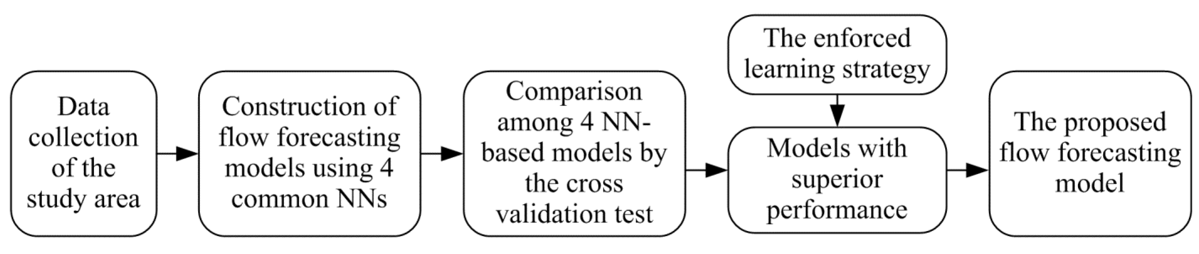
In this paper, to improve the hourly streamflow forecasting, a modeling methodology concerning the development of NN-based models with the enforced learning strategy is proposed. A flowchart of the development of the proposed NN-based flow forecasting model is presented in Figure 1.

Figure 1. Flowchart of the development of the proposed flow forecasting model.

Figure 1. Flowchart of the development of the proposed flow forecasting model.

2.1. Neural Networks

As shown in Figure 1, four NNs, which are commonly used for hydrological forecasting, are adopted to construct NN-based flow forecasting models in this study. Brief introductions of these NNs, namely BPN, RBFN, SOM and SVM, are provided below.

2.1.1. Back Propagation Neural Network

Back propagation neural network proposed by Rumelhart et al. [47] is the most commonly used for hydrological forecasting. The network typically consists of an input layer, one or more hidden layers of computation neurons, and an output layer. During the learning step, the input signals proceed through the network in a forward direction, and the error signal back propagates from the output layer toward the input layer. The objective of learning is to minimize the error function $F$:

$$F=\frac{1}{2}{\displaystyle {\sum }_{l=1}^L{(d_l-y_l)}^2}$$

(1)

where $d_l$ and $y_l$ are respectively the desired and the actual outputs for the lth sample. L is the total number of samples in the training data set. Mathematically, the $y_l$ resulting from a three-layer network with I input neurons, J hidden nodes, and one output neurons can be expressed as:

$$y_l=f\left({\displaystyle {\sum }_{j=1}^J{w}_j^{ho}f\left({\displaystyle {\sum }_{i=1}^I{w}_{ij}^{ih}{x}_{il}}\right)}\right)$$

(2)

where $x_{il}$ is the lth sample input to the ith neuron of the input layer, $w_{ij}^{ih}$ is the connection weight between the ith neuron of the input layer and the jth neuron of the hidden layer, $w_j^{ho}$ is the connection weight between the jth neuron of the hidden layer and the neuron of the output layer, and $f$ is the activation function. The most common form of $f$, i.e., the sigmoid function, is adopted herein. By using the back-propagation learning method, the connection weights are iteratively adjusted until the error function $F$ converges to an acceptable value. In this study, the network with one hidden layer is adopted. The number of hidden neurons is varied from one to 10 to select the most appropriate network architecture. For each number of hidden neurons, 30 different sets of initial connection weights are tried during the training process. The learning rate and the maximum training epoch are set to 0.8 and 10,000, respectively.

2.1.2. Radial Basis Function Neural Network

The radial basis function neural network developed by Broomhead and Lowe [48] has been widely employed in non-linear system identification and time series prediction because of its powerful ability of universal function approximation. An RBF network consists of an input layer, a hidden layer with a number of neurons, and an output layer. The hidden layer transforms data from the input space to the hidden space using a nonlinear function. The nonlinear function of hidden units is symmetric in the input space, and the output of each hidden neuron depends only on the radial distance between the input and the hidden neuron. The response of each hidden neuron is scaled by its connecting weight to the output neuron and then summed to produce the overall network output. Therefore, the output of RBFN is written as:

$$\widehat{y}=w_0+{\displaystyle {\sum }_{j=1}^M{w}_j{h}_j(x)}$$

(3)

where $w_j$ is the connecting weight between the jth hidden neuron and the output neuron, and $w_0$ is the bias. The values of $w_j$ and $w_0$ are estimated using the least mean square algorithm. $M$ is the number of hidden neurons. The $h_j(x)$ is the output of the jth hidden neuron given by:

$$h_j(x)=\exp \left(\frac{-1}{2{\text{ρ}}^2}{\Vert x-c_j\Vert }^2\right),j=1,2,\cdots ,M$$

(4)

where $\left|\right|\cdot \left|\right|$ denotes the Euclidean norm, $x$ is the input vector, $c_j$ is the center vector of the jth hidden neuron, and $\text{ρ}$ is the width of the hidden neurons. The value of $\text{ρ}$ can be calculated as $d_{\max }/\sqrt{2M}$, in which $d_{\max }$ is the maximum distance between two hidden neurons. As to the determination of the center vector of hidden neuron $c_j$, relevant works can be found in the literature (e.g., [19,20,24,49,50,51]). In this study, a simple method is applied. That is, the number of hidden neurons is set to 30 and the center vectors of these hidden neurons are selected randomly from the training data set. Moreover, to avoid the local optimal problem, a total of 30 sets of different selections of the center vectors are tried.

2.1.3. Support Vector Machine

Support vector machine, which is a novel kind of NN, is developed by Vapnik [52]. SVM is constructed based on both the structural risk minimization principle and the empirical risk minimization principle. This enables SVM to generalize well. Hence, SVM has emerged as an alternative tool in many conventional NNs dominated fields, especially for hydrological forecasting. Herein, a brief introduction of SVM is presented. More mathematical details can be found in several textbooks [52,53,54]. Based on $N_d$ training data, the objective of the SVM learning is to find a non-linear regression function to yield the output $\widehat{y}$, which is the best approximation of the desired output $y$ with an error tolerance of $\text{ε}$. The regression function that relates the input vector $x$ to the output $\widehat{y}$ can be written as:

$$f(x)=w^{\text{T}}\text{φ}(x)+b=\widehat{y}$$

(5)

where $\text{φ}(x)$ is a non-linear function mapping input vector $x$ to a high-dimensional feature space. w and $b$ are weights and bias, respectively, and can be estimated by minimizing the following structural risk function:

$$R=\frac{1}{2}{w}^{\text{T}}w+C{\displaystyle \sum _{i=1}^{N_d}{L}_{\text{ε}}({\widehat{y}}_i)}$$

(6)

where $C$ is a user-defined parameter representing the trade-off between the model complexity and the empirical error, and $L_{\text{ε}}$ is the Vapnik’s $\text{ε}$-insensitive loss function. Vapnik [52] transformed the SVM problem as an optimization problem:

$$\begin{array}{l}\text{Maximize }{\displaystyle \sum _{i=1}^{N_d}{y}_i({\alpha }_i-{{\alpha }^{\prime }}_i)}-\epsilon {\displaystyle \sum _{i=1}^{N_d}({\alpha }_i+{{\alpha }^{\prime }}_i)-}\frac{1}{2}{\displaystyle \sum _{i=1}^{N_d}{\displaystyle \sum _{j=1}^{N_d}({\alpha }_i-{{\alpha }^{\prime }}_i)({\alpha }_j-{{\alpha }^{\prime }}_j)\phi {(x_i)}^{\text{T}}}\phi (x_j)}\hfill \\ \text{subject to }{\displaystyle \sum _{i=1}^{N_d}({\alpha }_i-{{\alpha }^{\prime }}_i)=0}\hfill \\ \text{ 0}\le {\alpha }_i,{{\alpha }^{\prime }}_i\le C,i=1,2,\mathrm{...},N_d\hfill \end{array}$$

(7)

where $\text{α}$ and ${\alpha }^{\prime }$ are the dual Lagrange multipliers. The solution to Equation (7) is guaranteed to be unique and globally optimal because the objective function is a convex function. The optimal Lagrange multipliers ${\text{α}}^{*}$ are solved by the standard quadratic programming algorithm. Then, the regression function can be rewritten as:

$$f(x)={\displaystyle \sum _{i=1}^{N_d}{\alpha }_i^{*}\phi {(x_i)}^{\text{T}}\phi (x)+b}={\displaystyle \sum _{i=1}^{N_d}{\alpha }_i^{*}K(x_i,x)+b}$$

(8)

where $K(x_i,x)$ is the kernel function. The most used kernel function, i.e., the radial basis function, is adopted herein. Some of solved Lagrange multipliers $(\text{α}-{\alpha }^{\prime })$ are zero and should be eliminated from the regression function. The regression function involves the nonzero Lagrange multipliers and the corresponding input vectors of the training data, which are called the support vectors. The final regression function can be rewritten as:

$$f(x)={\displaystyle \sum _{k=1}^{N_{\text{sv}}}{\text{α}}_{k}K(x_k,x)+b}$$

(9)

where $x_k$ denotes the $k$th support vector and $N_{\text{sv}}$ is the number of support vectors. Herein, the parameter $C$, which means the trade-off between the model complexity and the empirical error, is set to 1. That means the model complexity is as important as the empirical error. In addition, it is acceptable to set the error tolerance $\text{ε}$ to 1% for flow forecasting.

2.1.4. Self-Organizing Map

The self-organizing map proposed by Kohonen is a special class of NN. In an unsupervised manner, the learning of SOM is to define the weights so that the mapping is ordered and descriptive of the distribution of input data [55]. Therefore, the SOM is capable of clustering, classification, estimation, and data mining. Additionally, the SOM can provide features that facilitate insight into the hydrological processes and has been used for hydrological forecasting. An SOM network consists of one input layer and one output layer, i.e., the Kohonen layer, with numerous neurons. Each neuron of the Kohonen layer has a synaptic weight vector having the same dimension as the input vector.

In this paper, the self-organizing linear output map (SOLO) proposed by Hsu et al. [37] is adopted to develop a flow forecasting model. The development of SOLO includes two steps: to classify the inputs using SOM and then to map the inputs into the outputs using multivariate linear regressions. In other words, SOLO uses piecewise linear regression functions to descript the nonlinear relationships between inputs and outputs. For example, if a $N\times N$ SOM is used to analyze the input data, then the input-output function mapping is therefore accomplished by a set of $N\times N$ piecewise linear regression functions that cover the entire input domain. For a certain input data $x$ belonging to the $i$th neuron, the output of SOLO is:

$$\widehat{y}=f_i(x)={\displaystyle \sum a^{i}x}+b_0^i,i=1,\mathrm{...},N\times N$$

(10)

where $a$ is the vector of regression parameters and $b_0$ is the bias. As reported by Hsu et al. [34], the structure of SOLO has been designed for rapid, precise, and inexpensive estimation of network parameters and system outputs. In this study, to reach a just conclusion, different dimensions ($N\times N,N=2,\text{ 3, 4, 5}$) are tried. The parameters of Equation (10) are decided by the least mean square algorithm.

2.2. Enforced Learning Strategy

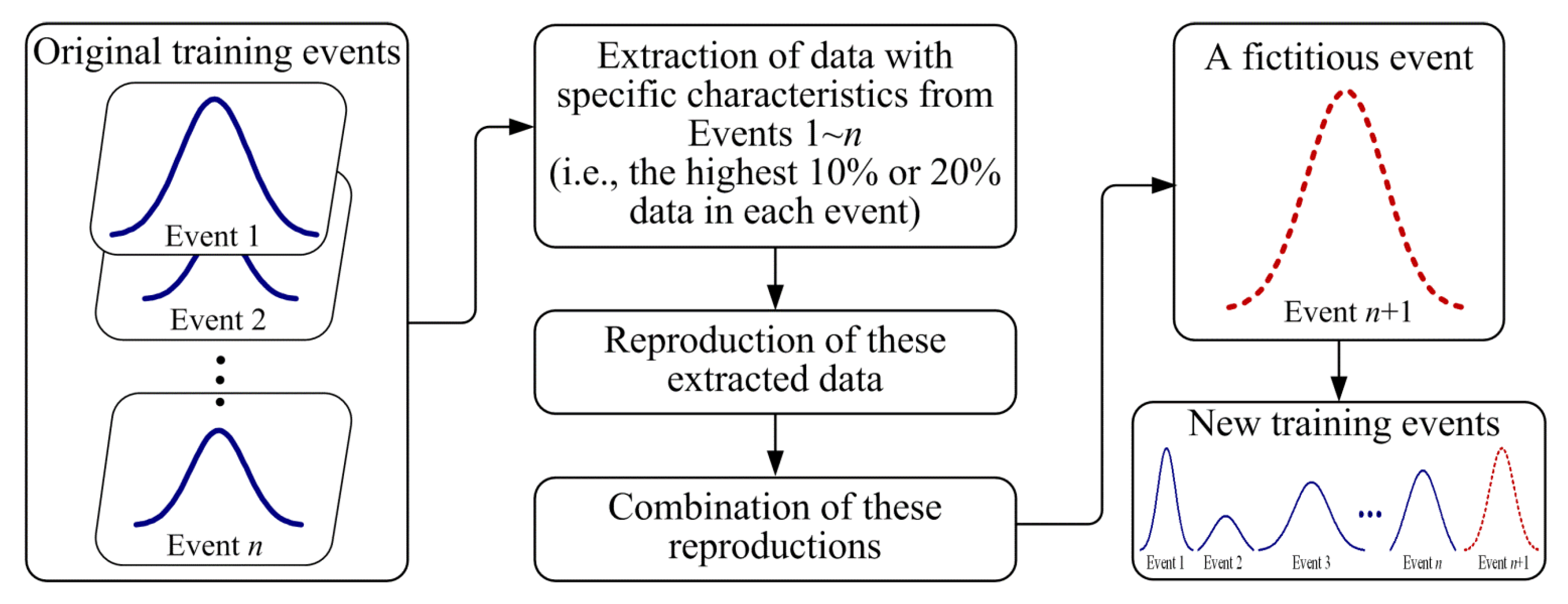
In order to improve the performance of NN-based forecasting models, an enforced learning strategy is proposed herein. Because NNs are nonlinear data-driven techniques, both the quantity and the quality of data available have great influence on the modeling performance [1]. During the training of NNs, the weights are adjusted iteratively to minimize the overall error between the desired and the actual outputs. Owing to the fact that the data of peak flow are insufficient in size, NN-based models are usually unable to yield satisfactory solutions of extreme values in the river flow [43]. The idea to increase the rate of the data with specific characteristics in the entirety of the learning data is applied. This idea is close to the human learning process. When we try to grasp specific and important information, we tend to practice repeatedly for better results [45,56]. Hence, in this study, a simple and quick data processing procedure is used. Firstly, the data with special characteristics, i.e., high-flow data herein, are extracted. At the present stage, based on authors’ experience, the highest 10% or 20% of data in each event are regarded as the data with specific characteristics. For a certain training event, if the peak flow is relatively high among all events, the highest 20% of all flow data in this event are extracted. Otherwise, the highest 10% of flow data are extracted. Second, these extracted high-flow data are directly reproduced. The corresponding rainfall data are also reproduced. Then, a fictitious event is generated by recombining these reproductions in a manner similar to the ranking method commonly used in the construction of design hyetographs [57]. This event is regarded as a new event and finally involved in the original training data for constructing NN-based models. An illustration of the aforementioned description is presented in Figure 2. It should be noted that the enforced learning strategy is used to process the original training data. By means of the enforced learning strategy, the training events are enhanced. The inputs, the original structure, and the parameters of NNs are not changed. The effectiveness of the enforced learning strategy can finally be drawn by comparing the NN-based models with and without the enforced learning strategy.

Figure 2. Graphical illustration of the enforced learning strategy.

Figure 2. Graphical illustration of the enforced learning strategy.

3. Application and Result Discussion

3.1. The Study Area and Data

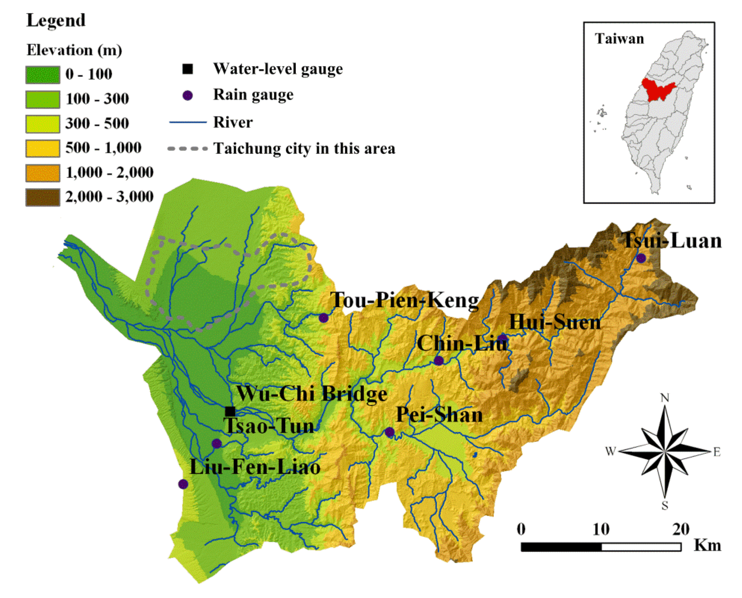
The study area of this paper is the Wu River basin located in central Western Taiwan. The lengths of the Wu River basin are 52 km in the north-south direction and 84 km in the east-west direction. The basin, with an area of 2026 km², ranks 4th in Taiwan. The length of the main river is 119 km, and the average slope is 1/92. In this basin, floods caused by heavy rainfalls are quite common. The metropolis of Taichung, which is a major city with a population of about three million in central Taiwan, is located downstream in the study area. Therefore, an accurate, efficient and robust flow forecasting model is needed for the study area.

As shown in Figure 3, there are seven rain gauges (Liu-Fen-Liao, Pei-Shan, Tsao-Tun, Chin-Liu, Hui-Suen, Tsui-Luan and Tou-Pien-Keng) and one water-level gauge (Wu-Chi Bridge) in the study area.

Figure 3. The study area and locations of rainfall and water level gauging stations.

Figure 3. The study area and locations of rainfall and water level gauging stations.

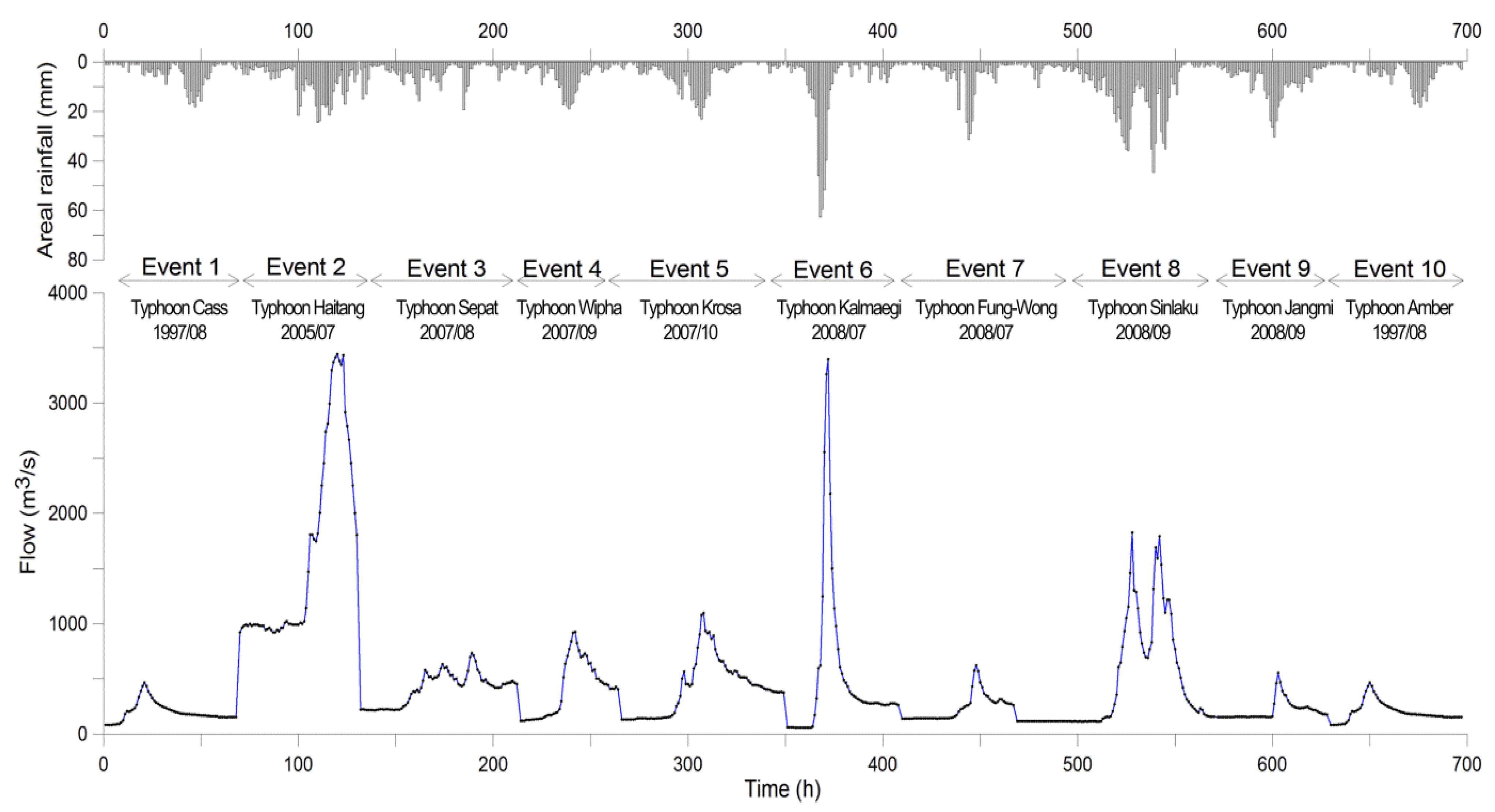
The observed rainfall and flow data are collected from the computer archives of the Water Resources Agency, Taiwan. These data are hourly values. Heavy rainfall events with rainfall and flow data available simultaneously are collected. Moreover, events under the condition that the basin is without any extensive development or land cover change are suggested. Hence, a total of 10 typhoon events with a length of approximately 700 hourly data are used in this study. In Figure 4, the areal rainfall and the corresponding flows, as well as the information of these 10 typhoon events are presented.

Figure 4. The areal rainfall and flow data used in this study.

Figure 4. The areal rainfall and flow data used in this study.

3.2. Input Design and Parameter Setting of NN-Base Models

In the construction of NN-based models, the input determination is critical. Generally, the inputs of NN-based flow forecasting models are antecedent flow and rainfall. Therefore, in this study these two hydrological variables are used and the work of input design is to select the best lag length in this study area. Herein, the canonical correlation analysis is adopted. The correlation between input and output time-series data is calculated using the Pearson product-moment correlation coefficient written as:

$$\rho =\frac{\mathrm{cov}(x,y)}{{\text{σ}}_x{\text{σ}}_y}$$

(11)

where $x$ and $y$ are the input and output time-series data, respectively. The larger value of $\text{ρ}$ means the higher correlation between $x$ and $y$. It is expected that the input, which has a higher correlation with the output, is helpful for forecasting the output. The $\text{ρ}$ between the antecedent rainfall with different time lags and the flow with a lead time of 1 h are calculated. The result summarized in Table 1 shows the $Q_{t+1}$ (where $t$ is the current time) has the highest correlation with $R_{t-2}$. This indicates the concentration time of the study area is about 3 h. Hence, the forecasting lead-time should not exceed 3 h in this study. Additionally, it is observed that the $Q_{t+1}$ has the highest correlation with $Q_t$ and $Q_{t-1}$. Therefore, according to Table 1, the best inputs of the NN-based model are decided and can then be written in a general form as:

$$Q_{t+i}=f(R_{t+i-3},Q_t,Q_{t-1}),i=1,2,3$$

(12)

where $R_{t+i-3}$ is the areal rainfall at time $t+i-3$, $Q_t$, $Q_{t-1}$ and $Q_{t+i}$ are flow at time $t$, $t-1$ and $t+i$, respectively. It should be noted that herein the best inputs mean the best lag length of input variables, which is influenced by the hydrological environment of the study area. Therefore, in this study, inputs of four NN-based flow forecasting models are all the same.

Table 1. Values of Pearson product-moment correlation coefficient.

Lag Length $j$	Pearson Product-Moment Correlation Coefficient $\text{ρ}$
	Between $Q_{t+1}$ and $R_{t-j}$	Between $Q_{t+1}$ and $Q_{t-j}$
0	0.48	0.95
1	0.55	0.88
2	0.58	0.80
3	0.56	0.72
4	0.52	0.65
5	0.46	0.58

Table 1. Values of Pearson product-moment correlation coefficient.

Lag Length $j$	Pearson Product-Moment Correlation Coefficient $\text{ρ}$
	Between $Q_{t+1}$ and $R_{t-j}$	Between $Q_{t+1}$ and $Q_{t-j}$
0	0.48	0.95
1	0.55	0.88
2	0.58	0.80
3	0.56	0.72
4	0.52	0.65
5	0.46	0.58

After the determination of model inputs, the parameter setting is then proceeded by trial and error. Finally, the BPN with one hidden layer included two neurons, the RBFN with 30 hidden neurons, and the SOM of the dimension of 3 × 3 are adopted in this study. To avoid the overtraining problem, the cross-validation test is adopted to evaluate the overall performance of NNs in this manuscript. Besides, a total of 30 repeats of NN learning are performed. Each NN is evaluated based on the mean performance of these 30 repeats, instead of the performance of only one learning. Hence, in this manner, the effect of overtraining on the training performance should be reduced and a just conclusion can be reached.

3.3. Cross Validation and Performance Measures

During the construction of NN-based models, the collected data are usually partitioned into two parts: training and testing. Training data are used to determine the architectures of NNs and adjust the weights of NN-based models. The performance of the trained NN-based models is then tested by the remaining data (i.e., testing data) that are not used in the training step. However, different selections of training and testing events may yield different results and sometimes lead to different conclusions. To reach just conclusions, cross validations are conducted herein. That is, each single event is used in turn as the testing event and the remaining events are used as training events. Thus, a total of 10 tests corresponding to 10 heavy rainfall events will be performed.

To evaluate the forecasting performance of each test, four performance measures are employed. Firstly, the relative root mean square error (RRMSE) is used. For a single event, the RRMSE is defined as:

$$RRMSE=\sqrt{\frac{1}{n}{\displaystyle {\sum }_{t=1}^n{\left(\frac{{\widehat{Q}}_t-Q_t}{Q_t}\right)}^2}}$$

(13)

where ${\widehat{Q}}_t$ and $Q_t$ are the forecasted and observed flows at time t, respectively, and n is the number of data points. For a total of N testing events, the mean RRMSE (MRRMSE) is then calculated. Second, the coefficient of efficiency (CE) is used [58,59]. For a single event, the CE is written as:

$$CE=1-\frac{{\displaystyle {\sum }_{t=1}^n{(Q_t-{\widehat{Q}}_t)}^2}}{{\displaystyle {\sum }_{t=1}^n{(Q_t-\overline{Q})}^2}}$$

(14)

where $\overline{Q}$ is the average of observed flow. The CE is often used to assess the forecasting ability of hydrological models. If the forecasts are perfect, the CE value is equal to one. For N testing events, the mean CE (MCE) is calculated. Third, the error of time to peak flow (ET_p) is used. For a single typhoon event, the ET_p is written as:

$$E{T}_P=\text{abs}({\widehat{T}}_p-T_p)$$

(15)

where ${\widehat{T}}_p$ and $T_P$ are the time to peak for forecasted and observed flows, respectively, and $\text{abs}()$ denotes the absolute value. For N typhoon events, the mean ET_p (MET_p) is calculated. Moreover, the percentage error of peak flow (EQ_p) is used. For a single typhoon event, the EQ_p is written as:

$$E{Q}_P=\text{abs}({\widehat{Q}}_p-Q_p)/Q_p\times 100$$

(16)

where ${\widehat{Q}}_p$ and $Q_P$ are the forecasted and observed peak flows, respectively. For N typhoon events, the mean EQ_p (MEQ_p) is calculated.

These four criteria adopted herein are the most commonly used in hydrology for assessing the forecasting performance. The RRMSE represents the relative error between the observed and forecasted flows. The CE, namely the Nash-Sutcliffe efficiency, represents the forecasting efficiency. The above two criteria are used to assess the overall forecasting performance. As to the specific fragment, the ET_p, and EQ_p are used to measure the forecasting error related to the peak values. Moreover, since the cross-validation test is used in this paper, the mean values of these four criteria (i.e., MRRMSE, MCE, MET_p, and MEQ_p) are further used to compare the forecasting performance of different NNs. Hence, based on the use of these criteria, a just conclusion is expected to be reached.

3.4. Performance Comparisons among Four NN-Based Models

Firstly, we focus on the accuracy of four NN-based models. Four performance measures are calculated and presented in Table 2. As shown in Table 2, the MRRMSE, MET_p, and MEQ_p values increase with increasing forecast lead time, and the MCE values decrease with increasing forecast lead time. It is observed that the SOLO and the SVM models yield lower MRRMSE values and higher CE values than the BPN and the RBFN models for 1- to 3-h ahead forecasting. The results indicate the SOLO and the SVM models perform better than the BPN and the RBFN models. As to the comparison between the SOLO and the SVM models, the SOLO model performs better than the SVM model for 1-h ahead forecasting. For 2-h ahead forecasting, these two models perform equally well, and for 3-h ahead forecasting the SVM model performs better than the SOLO model. It may be speculated that for 1-h ahead forecasting the relation between rainfall and flow is slightly nonlinear, and hence the piecewise linear model (i.e., SOLO) quickly captures the relationship hidden in the training data and yields better forecasts as compared to the nonlinear model (i.e., SVM). For 3-h ahead forecasting the relation between rainfall and flow is very complicated and highly nonlinear, and therefore the SVM model performs better than the SOLO model. As to the MET_p and MEQ_p values, the SOLO model yields the lowest MET_p, while the SVM gives the lowest MEQ_p. Overall, it is concluded that the forecasts resulting from the SOLO and the SVM models are more accurate than those from the other two models in this study. Among these four models, the forecasting performance of the RBFN model is the worst. For 3-h ahead forecasting, the CE value from the RBFN model is even negative. That indicates the observed mean is a better forecast than the output of the RBFN model. Maybe the random selection procedure used herein cannot effectively obtain the best center vectors of RBFN hidden neurons.

Table 2. Results of four NN-based flow forecasting models.

Model	MRRMSE (%)			MCE			METp (h)			MEQP (%)
	1-h ahead	2-h ahead	3-h ahead	1-h ahead	2-h ahead	3-h ahead	1-h ahead	2-h ahead	3-h ahead	1-h ahead	2-h ahead	3-h ahead
BPN	26.5	32.2	44.5	0.83	0.57	0.15	2.1	2.8	3.9	10.6	18.2	28.1
RBFN	15.4	32.0	42.2	0.87	0.48	−0.11	2.2	2.8	4.5	9.9	24.6	37.7
SOLO	9.1	19.0	28.8	0.94	0.72	0.34	0.7	1.3	2.2	8.8	16.5	23.1
SVM	12.1	18.8	27.5	0.90	0.72	0.47	2.1	2.8	2.7	7.2	12.9	18.6

Notes: MRRMSE is the mean relative root mean square error; MCE is the mean coefficient of efficiency; MET_p is the mean error of time to peak flow; MEQ_p is the mean error of peak flow.

Table 2. Results of four NN-based flow forecasting models.

Model	MRRMSE (%)			MCE			METp (h)			MEQP (%)
	1-h ahead	2-h ahead	3-h ahead	1-h ahead	2-h ahead	3-h ahead	1-h ahead	2-h ahead	3-h ahead	1-h ahead	2-h ahead	3-h ahead
BPN	26.5	32.2	44.5	0.83	0.57	0.15	2.1	2.8	3.9	10.6	18.2	28.1
RBFN	15.4	32.0	42.2	0.87	0.48	−0.11	2.2	2.8	4.5	9.9	24.6	37.7
SOLO	9.1	19.0	28.8	0.94	0.72	0.34	0.7	1.3	2.2	8.8	16.5	23.1
SVM	12.1	18.8	27.5	0.90	0.72	0.47	2.1	2.8	2.7	7.2	12.9	18.6

Notes: MRRMSE is the mean relative root mean square error; MCE is the mean coefficient of efficiency; MET_p is the mean error of time to peak flow; MEQ_p is the mean error of peak flow.

Second, we focus on the robustness of these four NN-based models. To construct a robust NN-based model that can yield reliable forecasts, a robust weight optimization algorithm is important. For a robust optimization algorithm, the obtained optimal weights should slightly be influenced by the selections of initial weights. On the contrary, the optimization algorithm is less robust if obtained optimal weights are highly dependent on the initial weights. To demonstrate the robustness of these four models, an experiment that 30 repeats of each model under the same model inputs and architecture is executed herein. Hence, 30 MCE values are obtained for each model. Then, the lack of robustness can be evaluated by the variation in MCE values. The coefficient of variation (CV), which is calculated by dividing the standard deviation with the mean, is used herein. A higher CV value of MCE represents the higher variation in MCE and also indicates that the performance of the corresponding model is less reliable. The CV values listed in Table 3 are calculated from a data set of 30 MCE values. As shown in Table 3, the CV values resulting from the SOLO and SVM models are zero. That is, SOLO and SVM models yield a constant MCE value in 30 runs. As to the RBFN and BPN models, different initial weights lead to different MCE values even when the same training and testing data are used. Table 3 clearly shows that the robustness of the SOLO and SVM models are better than that of RBFN and BPN models. The obtained optimal weights of the SOLO and SVM models are not influenced by the selections of initial weights. The forecasts resulting from the SOLO and SVM models are more reliable than those from the RBFN and BPN models. Hence, according to the model accuracy and the model robustness (i.e., the results in Table 2 and Table 3), it is concluded that the SOLO and SVM models are the best two among the four NN-based models in this study. Consequently, the SOLO and SVM models are then used in the following section to evaluate the effect of the enforced learning strategy on NN-based models for developing the proposed flow forecasting models.

Table 3. CV values resulting from various NN-based models.

Lead Time (h)	CV (%)
	BPN	RBFN	SOLO	SVM
1	0.1	2.4	0	0
2	0.3	23.1	0	0
3	16.1	−151.7	0	0

Note: Coefficient of variation (CV) is calculated from a data set of 30 CE values resulting from each model trained with 30 different sets of initial weights.

Table 3. CV values resulting from various NN-based models.

Lead Time (h)	CV (%)
	BPN	RBFN	SOLO	SVM
1	0.1	2.4	0	0
2	0.3	23.1	0	0
3	16.1	−151.7	0	0

Note: Coefficient of variation (CV) is calculated from a data set of 30 CE values resulting from each model trained with 30 different sets of initial weights.

3.5. Effects of the Enforced Learning Strategy on NN-Based Models

For further improving the performance of SOLO and SVM, which are the superior NN-based forecasting models in this study, the enforced learning strategy is involved in the development of the SOLO and the SVM models. The comparisons of NN-based models with and without the enforced learning strategy are then executed to assess the effect of the enforced learning strategy on the NN-based models. It should be noted that the inputs, the architecture, and the parameter of these NN-based model are unchanged. Only the data used in the training step are different. By means of the enforced learning strategy, a fictitious event is added in the original training data for constructing the NN-based models. Additionally, in this section the enforced learning strategy is applied during the construction of two different NN-based models. Hence, a just conclusion regarding the effect of enforced learning strategy on NN-based models is expected to be reached.

3.5.1. Comparison of the SOLO Models with and without the Enforced Learning Strategy

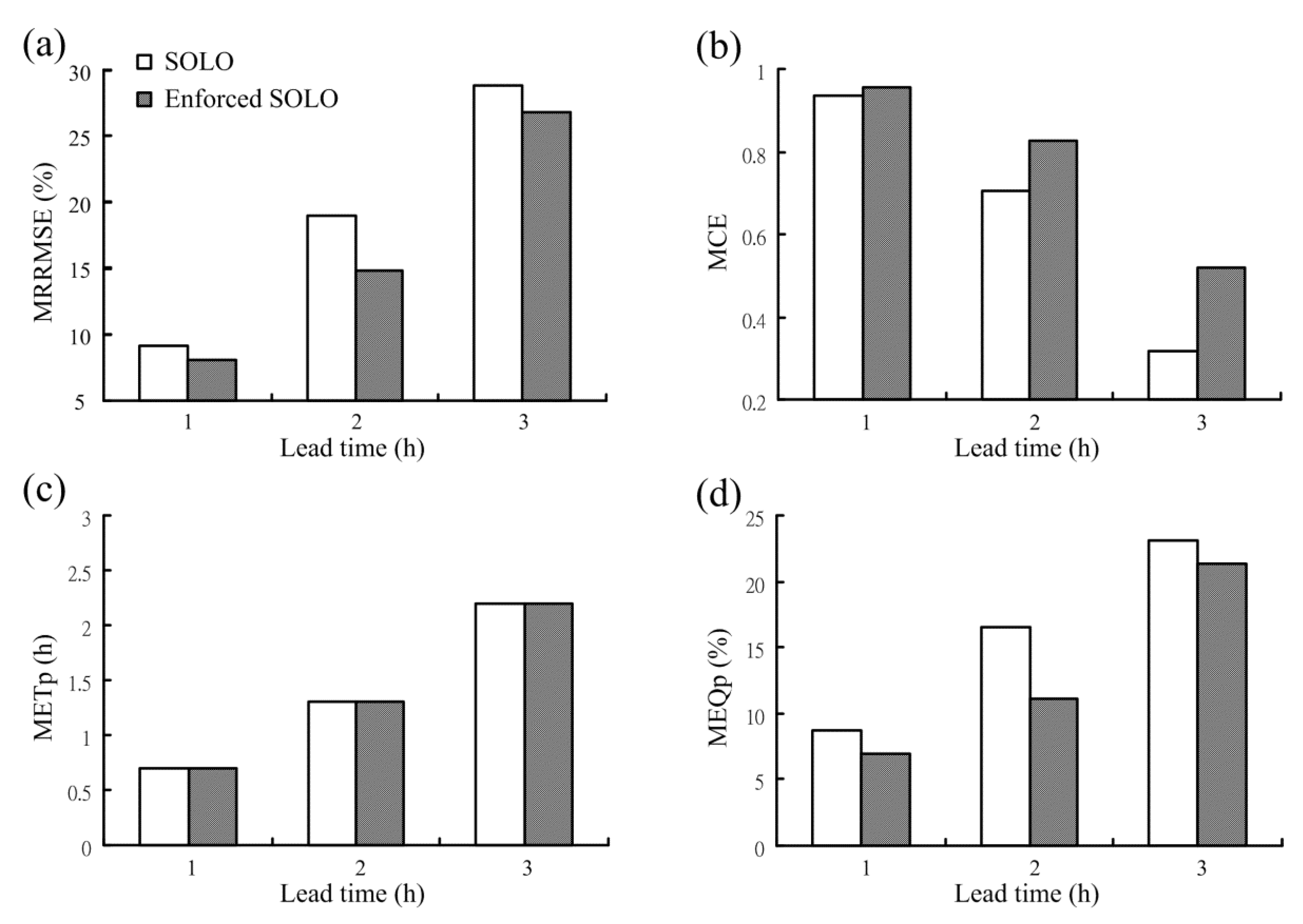
In this subsection, the influence of the enforced learning strategy on the SOLO model is discussed. In contrast to the SOLO model constructed earlier, the SOLO model constructed with the enforced learning strategy is named the enforced SOLO model hereafter. The enforced SOLO model is also applied to forecast the streamflow with a lead time of 1- to 3-h. The bar charts corresponding to four performance measures from the SOLO and the enforced SOLO models are presented in Figure 5. As shown in Figure 5, the enforced SOLO model yielded lower MRRMSE and higher MCE values than the SOLO model. That is, the enforced SOLO model provides more accurate forecasts as compared to the SOLO model. As to the peak flow forecasting, the MEQ_p values from the enforced SOLO model are lower than those from the SOLO model. As to MET_p, the performance of the SOLO and the enforced SOLO models are the same. That is, the enforced SOLO model also provides more accurate forecasts for the peak flow.

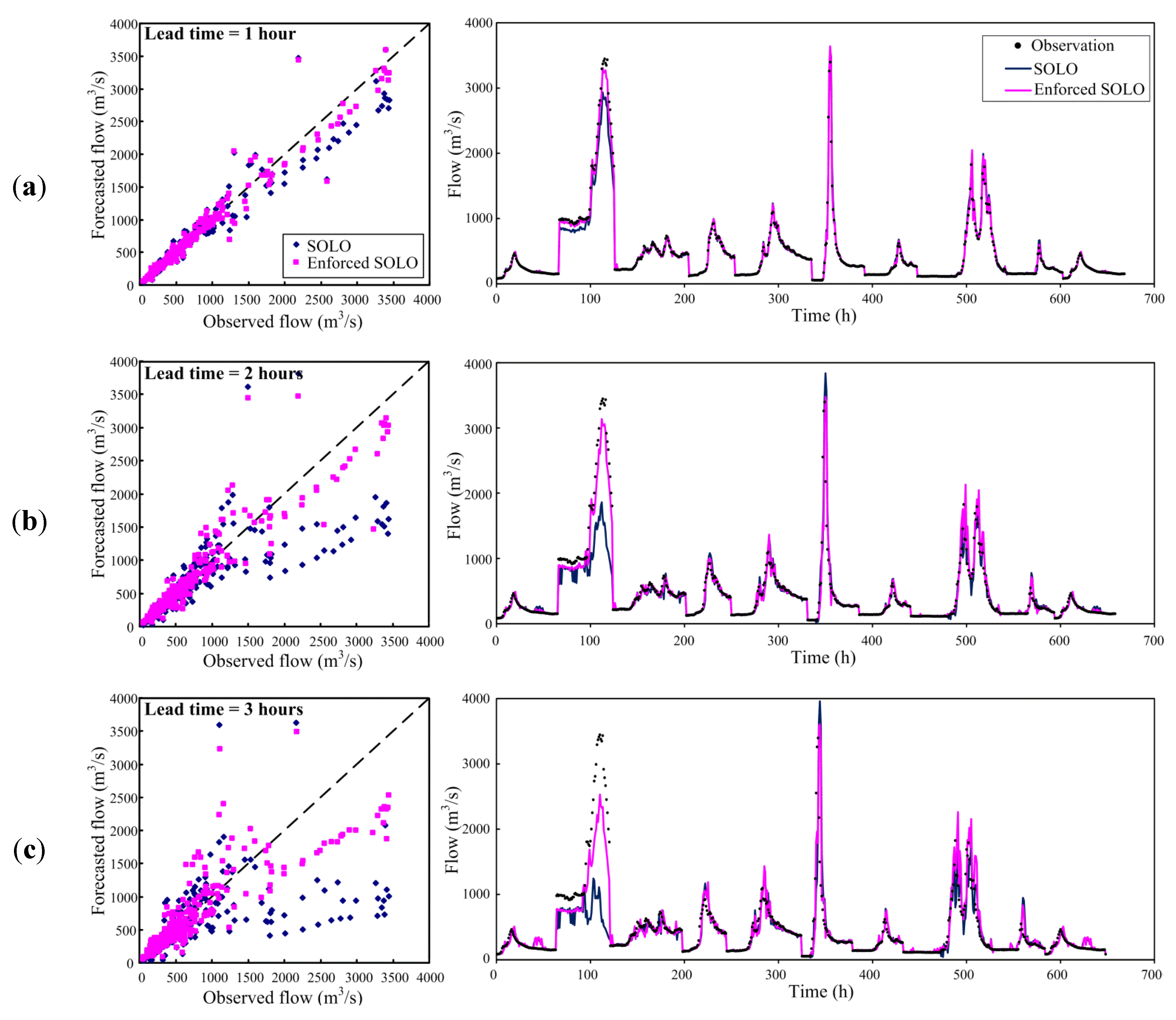
Moreover, the observed flows versus corresponding forecasts resulting from the SOLO and from the enforced SOLO models are presented. The scatter plots and the forecasted hydrographs for 1- to 3-h ahead forecasting are shown in Figure 6. It is observed that the forecasts from the enforced SOLO are in better agreement with the observations as compared to those from the SOLO. Therefore, Figure 6 again confirms that the enforced SOLO model indeed provides improved forecasts as compared to the SOLO model. Furthermore, to show the superiority of the enforced SOLO model more clearly the events (Events 2 and 6), which yielded the maximum peak flows in our used data are highlighted. On average, the EQ_P values of the SOLO model are 12%, 27% and 55% for 1- to 3-h ahead forecasting. By using the enforced SOLO model, these corresponding EQ_P values are 6%, 11% and 37%. A significant improvement in reducing the error of peak flow forecasting is clearly observed. Hence, according to the comparison results above, it is clearly concluded that the improved streamflow forecasts are indeed obtained by the enforced SOLO model (i.e., the SOLO model with the enforced learning strategy).

Figure 5. Performance comparison of the SOLO and the enforced SOLO models: (a) MRRMSE; (b) MCE; (c) MET_p and (d) MEQ_p.

Figure 5. Performance comparison of the SOLO and the enforced SOLO models: (a) MRRMSE; (b) MCE; (c) MET_p and (d) MEQ_p.

3.5.2. Comparison of the SVM Models with and without the Enforced Learning Strategy

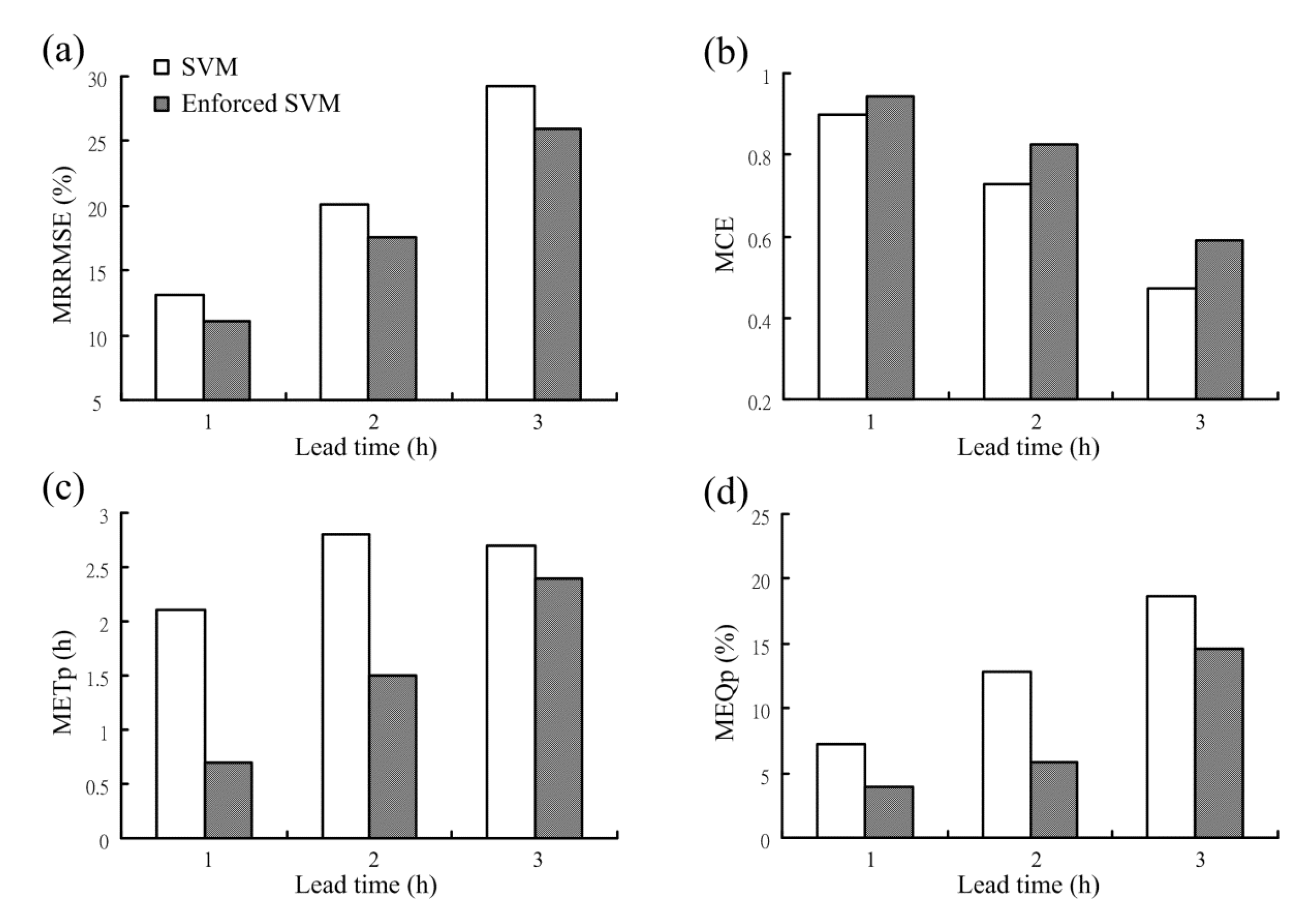
In this subsection, the influence of the enforced learning strategy on another NN-based model, i.e., the SVM model, is discussed. The SVM model with the enforced learning strategy is named the enforced SVM model hereafter. Four performance measures resulting from the SVM and the enforced SVM models are graphically displayed in Figure 7. The results in Figure 7 show that as compared to the SVM model, the enforced SVM model provides the forecasts with lower MRRMSE values and the higher MCE values. Moreover, the MET_p and MEQ_p values from the enforced SVM model are lower than those from the SVM model. It is concluded that the enforced SVM model indeed improves the forecasts of overall flows as well as the peaks, and the enforced learning strategy successfully improves the forecasting performance of the SVM model.

Figure 6. Observed flows versus corresponding forecasts resulting from the SOLO and the enforced SOLO models: (a) 1-h ahead; (b) 2-h ahead and (c) 3-h ahead.

Figure 6. Observed flows versus corresponding forecasts resulting from the SOLO and the enforced SOLO models: (a) 1-h ahead; (b) 2-h ahead and (c) 3-h ahead.

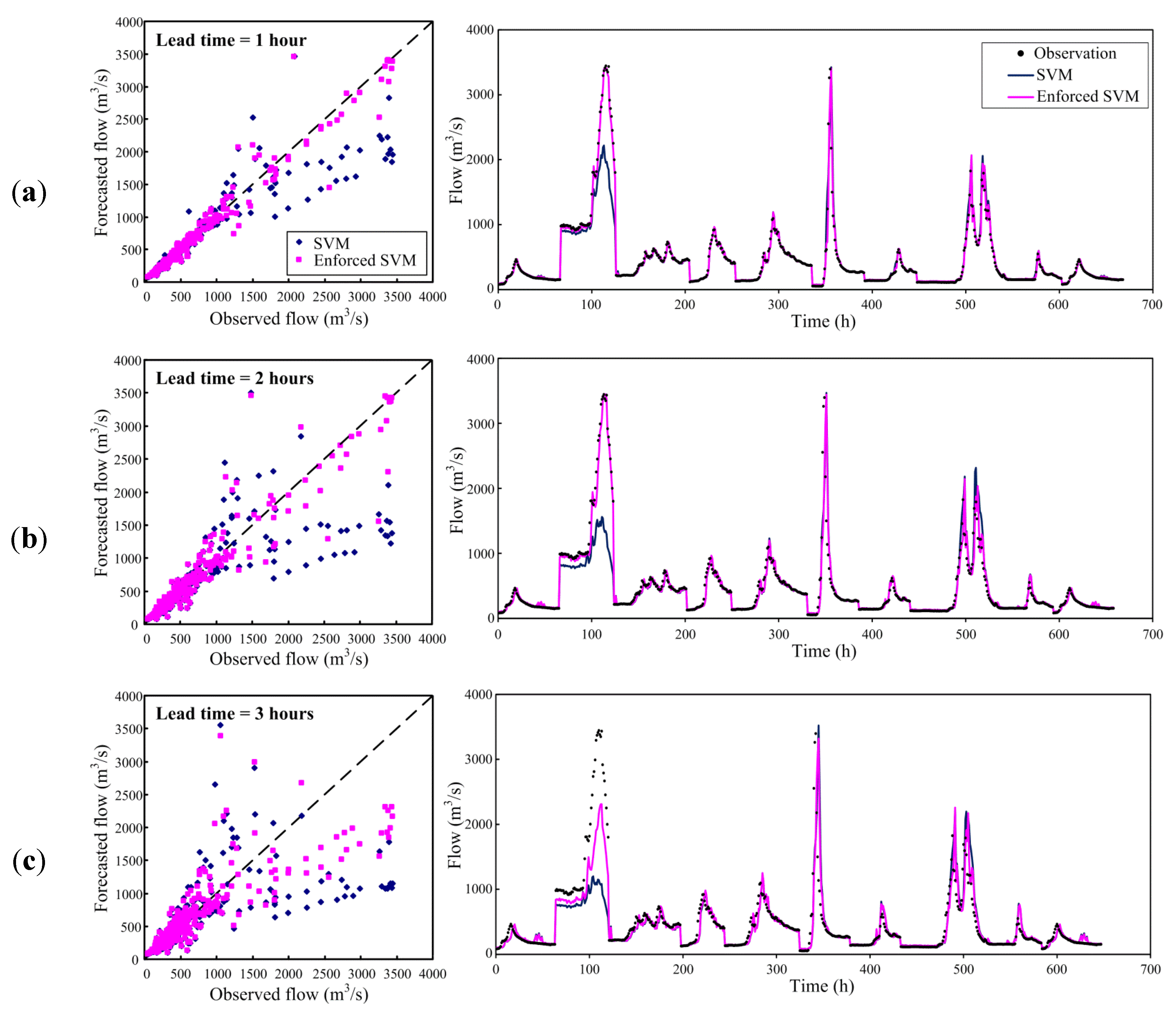
Figure 8 shows the observed flow versus corresponding forecasts from the SVM and the enforced SVM models. Again, Figure 8 confirms the enforced SVM model indeed provides improved forecasts of flows due to the better agreement between the observations and forecasts. Furthermore, the events that yielded the maximum peak flows in our data are focused to show the superiority of the enforced SVM model. On average, the EQ_P values of the SVM model are 30%, 49% and 58% for 1- to 3-h ahead forecasting. Those are reduced to 6%, 16% and 42% by means of the enforced SVM. Again, a significant improvement in reducing the error of peak flow forecasting is clearly observed. Hence, based on the results above, it is concluded that the improved forecasts are indeed obtained by using the enforced SVM model (i.e., the SVM model with the enforced learning strategy).

Due to the results concerning the comparison between the SOLO and the enforced SOLO and the comparison between the SVM and the enforced SVM, the use of the enforced learning strategy indeed let both the SOM and SVM provide improved forecasts. More accurate forecasts of overall streamflow as well as the peaks are obtained. That is, the enforced learning strategy is indeed helpful for improving the forecasting performance of NNs, even when different NNs are used.

Figure 7. Performance comparison of the SVM and the enforced SVM models: (a) MRRMSE; (b) MCE; (c) MET_p; and (d) MEQ_P.

Figure 7. Performance comparison of the SVM and the enforced SVM models: (a) MRRMSE; (b) MCE; (c) MET_p; and (d) MEQ_P.

Figure 8. Observed flows versus corresponding forecasts resulting from the SVM and the enforced SVM models: (a) 1-h ahead; (b) 2-h ahead and (c) 3-h ahead.

Figure 8. Observed flows versus corresponding forecasts resulting from the SVM and the enforced SVM models: (a) 1-h ahead; (b) 2-h ahead and (c) 3-h ahead.

4. Conclusions

To improve the performance of hourly flow forecasting, a methodology concerning the development of NN-based models with the enforced learning strategy is presented. Firstly, four common NNs (namely, BPN, BFN, SOLO and SVM) are used to construct NN-based flow forecasting models. Through the cross-validation test, it is observed that SOLO and SVM provide better and more robust forecasts than BPN and RBFN in our study. To further improve the performance of NN-based models, the enforced learning strategy is proposed. Therefore, the data with special characteristics (i.e., the peak flows herein) are reproduced and recombined to be a fictitious event. This event is regarded as new training data and used for constructing the SOLO and the SVM models. Comparisons between NN-based models with and without the enforced learning strategy are performed. The results show that the improved forecasts are obtained through the enforced NN-based models (i.e., the NN-based models constructed with the enforced learning strategy). Hence, it is confirmed that the enforced learning algorithm successfully improves the forecasting performance of the NN-based flow forecasting models. In conclusion, the proposed enforced NN-based model is recommended as an alternative to the existing NN-based models for flow forecasting. The presented methodology is also expected to be helpful for developing an NN-based forecasting model. Nevertheless, more applications of the methodology in different hydrologic environments should be conducted to further assess the methodology’s potential. Additionally, further study on improving the enforced learning strategy such as the objective determination of the data with special characteristics is still required in future research.

References

- ASCE Task Committee on Application of Artificial Neural Networks in Hydrology. Artificial Neural Networks in Hydrology, part I: Preliminary concepts. J. Hydrol. Eng. 2000, 5, 115–123. [Google Scholar] [CrossRef]
- ASCE Task Committee on Application of Artificial Neural Networks in Hydrology. Artificial Neural Networks in Hydrology, part II: Hydrologic applications. J. Hydrol. Eng. 2000, 5, 124–137. [Google Scholar] [CrossRef]
- Govindaraju, R.S.; Rao, A.R. Artificial Neural Networks in Hydrology; Kluwer: Alphen aan den Rijn, The Netherlands, 2000. [Google Scholar]
- Maier, H.R.; Dandy, G.C. Neural networks for the prediction and forecasting of water resources variables: A review of modelling issues and applications. Environ. Model. Softw. 2000, 15, 101–124. [Google Scholar] [CrossRef]
- Maier, H.R.; Jain, A.; Dandy, G.C.; Sudheer, K.P. Methods used for the development of neural networks for the prediction of water resource variables in river systems: Current status and future directions. Environ. Model. Softw. 2010, 25, 891–909. [Google Scholar] [CrossRef]
- Huang, W.; Xu, B.; Chan-Hilton, A. Forecasting flows in Apalachicola River using neural networks. Hydrol. Process. 2004, 18, 2545–2564. [Google Scholar] [CrossRef]
- Chau, K.W.; Wu, C.L.; Li, Y.S. Comparison of several flood forecasting models in Yangtze River. J. Hydrol. Eng. 2005, 10, 485–491. [Google Scholar] [CrossRef]
- Lin, G.F.; Chen, G.R. A systematic approach to the input determination for neural network rainfall-runoff models. Hydrol. Process. 2008, 22, 2524–2530. [Google Scholar] [CrossRef]
- Cheng, C.T.; Niu, W.J.; Feng, Z.K.; Shen, J.J.; Chau, K.W. Daily reservoir runoff forecasting method using artificial neural network based on quantum-behaved particle swarm optimization. Water 2015, 7, 4232–4246. [Google Scholar] [CrossRef]
- Xu, Z.X.; Li, J.Y. Short-term inflow forecasting using an artificial neural network model. Hydrol. Process. 2002, 16, 2423–2439. [Google Scholar] [CrossRef]
- Coulibaly, P.; Haché, M.; Fortin, V.; Bobée, B. Improving daily reservoir inflow forecasts with model combination. J. Hydrol. Eng. 2005, 10, 91–99. [Google Scholar] [CrossRef]
- Wu, C.L.; Chau, K.W. A flood forecasting neural network model with genetic algorithm. Int. J. Environ. Pollut. 2006, 28, 261–273. [Google Scholar] [CrossRef]
- Muluye, G.V.; Coulibaly, P. Seasonal reservoir inflow forecasting with low-frequency climatic indices: A comparison of data-driven methods. Hydrol. Sci. J. 2007, 52, 508–522. [Google Scholar] [CrossRef]
- Tayfur, G.; Moramarco, T.; Singh, V.P. Predicting and forecasting flow discharge at sites receiving significant lateral inflow. Hydrol. Process. 2007, 21, 1848–1859. [Google Scholar] [CrossRef]
- Lin, G.F.; Huang, P.Y.; Chen, G.R. Using typhoon characteristics to improve the long lead-time flood forecasting of a small watershed. J. Hydrol. 2010, 380, 450–459. [Google Scholar] [CrossRef]
- Taormina, R.; Chau, K.W. Neural network river forecasting with multi-objective fully informed particle swarm optimization. J. Hydroinform. 2015, 17, 99–113. [Google Scholar] [CrossRef]
- Wang, Y.; Guo, S.; Xiong, L.; Liu, P.; Liu, D. Daily runoff forecasting model based on ANN and data preprocessing techniques. Water 2015, 7, 4144–4160. [Google Scholar] [CrossRef]
- Dawson, C.W.; Harpham, C.; Wilby, R.L.; Chen, Y. Evaluation of artificial neural network techniques for flow forecasting in the River Yangtze, China. Hydrol. Earth Syst. Sci. 2002, 6, 619–626. [Google Scholar] [CrossRef]
- Lin, G.F.; Chen, L.H. A non-linear rainfall-runoff model using radial basis function network. J. Hydrol. 2004, 289, 1–8. [Google Scholar] [CrossRef]
- Lin, G.F.; Wu, M.C. An RBF network with a two-step learning algorithm for developing a reservoir inflow forecasting model. J. Hydrol. 2011, 405, 439–450. [Google Scholar] [CrossRef]
- Sahoo, G.B.; Raya, C. Flow forecasting for a Hawaii stream using rating curves and neural networks. J. Hydrol. 2006, 317, 63–80. [Google Scholar] [CrossRef]
- Sudheer, K.P.; Srinivasan, K.; Neelakantan, T.R.; Srinivas, V.V. A nonlinear data-driven model for synthetic generation of annual streamflows. Hydrol. Process. 2008, 22, 1831–1845. [Google Scholar] [CrossRef]
- Mutlu, E.; Chaubey, I.; Hexmoor, H.; Bajwa, S.G. Comparison of artificial neural network models for hydrologic predictions at multiple gauging stations in an agricultural watershed. Hydrol. Process. 2008, 22, 5097–106. [Google Scholar] [CrossRef]
- Chang, L.C.; Chang, F.J.; Wang, Y.P. Auto-configuring radial basis function networks for chaotic time series and flood forecasting. Hydrol. Process. 2009, 23, 2450–2459. [Google Scholar] [CrossRef]
- Lin, G.F.; Wu, M.C.; Chen, G.R.; Tsai, F.Y. An RBF-based model with an information processor for forecasting hourly reservoir inflow during typhoons. Hydrol. Process. 2009, 23, 3598–3609. [Google Scholar] [CrossRef]
- Liong, S.Y.; Sivapragasam, C. Flood stage forecasting with support vector machines. J. Am. Water Resour. Assoc. 2002, 38, 173–186. [Google Scholar] [CrossRef]
- Wu, C.L.; Chau, K.W.; Li, Y.S. River stage prediction based on a distributed support vector regression. J. Hydrol. 2008, 358, 96–111. [Google Scholar] [CrossRef]
- Wu, M.C.; Lin, G.F.; Lin, H.Y. Improving the forecasts of extreme streamflow by support vector regression with the data extracted by self organizing map. Hydrol. Process. 2014, 28, 386–397. [Google Scholar] [CrossRef]
- Yu, X.Y.; Liong, S.Y.; Babovic, V. EC-SVM approach for real-time hydrologic forecasting. J. Hydroinform. 2004, 6, 209–223. [Google Scholar]
- Sivapragasam, C.; Liong, S.Y. Flow categorization model for improving forecasting. Nordic Hydrol. 2005, 36, 37–48. [Google Scholar]
- Yu, X.Y.; Liong, S.Y. Forecasting of hydrologic time series with ridge regression in feature space. J. Hydrol. 2007, 332, 290–302. [Google Scholar] [CrossRef]
- Wang, W.C.; Chau, K.W.; Cheng, C.T.; Qiu, L. A comparison of performance of several artificial intelligence methods for forecasting monthly discharge time series. J. Hydrol. 2009, 374, 294–306. [Google Scholar] [CrossRef]
- Lin, G.F.; Chen, G.R.; Huang, P.Y.; Chou, Y.C. Support vector machine-based models for hourly reservoir inflow forecasting during typhoon-warning periods. J. Hydrol. 2009, 372, 17–29. [Google Scholar] [CrossRef]
- Lin, G.F.; Chen, G.R.; Huang, P.Y. Effective typhoon characteristics and their effects on SVM-based hourly reservoir inflow forecasting models. Adv. Water Resour. 2010, 33, 887–898. [Google Scholar] [CrossRef]
- Noori, R.; Karbassi, A.R.; Moghaddamnia, A.; Han, D.; Zokaei-Ashtiani, M.H.; Farokhnia, A.; Gousheh, M.G. Assessment of input variables determination on the SVM model performance using PCA, Gamma test, and forward selection techniques for monthly stream flow prediction. J. Hydrol. 2011, 401, 177–189. [Google Scholar] [CrossRef]
- Lin, G.F.; Chou, Y.C.; Wu, M.C. Typhoon flood forecasting using integrated two-stage support vector machine approach. J. Hydrol. 2013, 486, 334–342. [Google Scholar] [CrossRef]
- Hsu, K.L.; Gupta, H.V.; Gao, X.; Sorooshian, S.; Imam, B. Self-organizing linear output map (SOLO): An artificial neural network suitable for hydrologic modeling and analysis. Water Resour. Res. 2002, 38, 10–26. [Google Scholar] [CrossRef]
- Moradkhani, H.; Hsu, K.L.; Gupta, H.V.; Sorooshian, S. Improved streamflow forecasting using self-organizing radial basis function artificial neural networks. J. Hydrol. 2004, 295, 246–262. [Google Scholar] [CrossRef]
- Hong, Y.; Hsu, K.; Sorooshian, S.; Gao, X. Self-organizing nonlinear output (SONO): A neural network suitable for cloud patch-based rainfall estimation at small scales. Water Resour. Res. 2005, 41. [Google Scholar] [CrossRef]
- Chang, F.J.; Chang, L.C.; Wang, Y.S. Enforced self-organizing map neural networks for river flood forecasting. Hydrol. Process. 2007, 21, 741–749. [Google Scholar] [CrossRef]
- Yang, C.C.; Chen, C.S. Application of integrated back-propagation network and self-organizing map for flood forecasting. Hydrol. Process. 2009, 23, 1313–1323. [Google Scholar] [CrossRef]
- Kim, S.; Singh, V.P. Spatial disaggregation of areal rainfall using two different artificial neural networks models. Water 2015, 7, 2707–2727. [Google Scholar] [CrossRef]
- Sudheer, K.P.; Nayak, P.C.; Ramasastri, K.S. Improving peak flow estimates in artificial neural network river flow models. Hydrol. Process. 2003, 17, 677–686. [Google Scholar] [CrossRef]
- Venkatasubramanian, V. Drowning in data: Informatics and modeling challenges in a data-rich networked world. AICHE J. 2009, 55, 2–8. [Google Scholar] [CrossRef]
- Fu, L.T.; Kara, L.B. Neural network-based symbol recognition using a few labeled samples. Comput. Graph. UK 2011, 35, 955–966. [Google Scholar] [CrossRef]
- Chen, S.T. Mining informative hydrologic data by using support vector machines and elucidating mined data according to information entropy. Entropy 2015, 17, 1023–1041. [Google Scholar] [CrossRef]
- Rumelhart, D.E.; Hinton, G.E.; Williams, R.J. Learning Internal Representations by Error Propagation; MIT Press: Cambridge, MA, USA, 1986. [Google Scholar]
- Broomhead, D.S.; Lowe, D. Multivariable function interpolation and adaptive networks. Complex Syst. 1988, 2, 321–355. [Google Scholar]
- Lin, G.F.; Chen, L.H. Time series forecasting by combining the radial basis function network and the self-organizing map. Hydrol. Process. 2005, 19, 1925–1937. [Google Scholar] [CrossRef]
- Jayawardena, A.W.; Xu, P.C.; Tsang, F.L.; Li, W.K. Determining the structure of a radial basis function network for prediction of nonlinear hydrological time series. Hydrol. Sci. J. 2006, 51, 21–44. [Google Scholar] [CrossRef]
- Lin, C.L.; Wang, J.F.; Chen, C.Y.; Chen, C.W.; Yen, C.W. Improving the generalization performance of RBF neural networks using a linear regression technique. Expert Syst. Appl. 2009, 36, 12049–12053. [Google Scholar] [CrossRef]
- Vapnik, V.N. The Nature of Statistical Learning Theory; Springer: Berlin, Germany, 1995. [Google Scholar]
- Vapnik, V.N. Statistical Learning Theory; John Wiley: New York, NY, USA, 1998. [Google Scholar]
- Cristianini, N.; Shaw-Taylor, J. An Introduction to Support Vector Machines and Other Kernel-Based Learning Methods; Cambridge University Press: New York, NY, USA, 2000. [Google Scholar]
- Kohonen, T. Self-Organizing Maps; Springer-Verlag: Berlin, Germany, 2001. [Google Scholar]
- Tserng, H.P.; Lin, G.F.; Tsai, L.K.; Chen, P.C. An enforced support vector machine model for construction contractor default prediction. Autom. Constr. 2011, 20, 1242–1249. [Google Scholar] [CrossRef]
- Kimura, N.; Tai, A.; Chiang, S.; Wei, H.P.; Su, Y.F.; Cheng, C.T.; Kitoh, A. Hydrological flood simulation using a design hyetograph created from extreme weather data of a high-resolution atmospheric general circulation model. Water 2014, 6, 345–366. [Google Scholar] [CrossRef]
- Nash, J.E.; Sutcliffe, J.V. River flow forecasting through conceptual models, Part 1: A discussion of principles. J. Hydrol. 1970, 10, 282–290. [Google Scholar] [CrossRef]
- Gupta, H.V.; Kling, H.; Yilmaz, K.K.; Martinez, G.F. Decomposition of the mean squared error and NSE performance criteria: Implications for improving hydrological modeling. J. Hydrol. 2009, 377, 80–91. [Google Scholar] [CrossRef]
© 2015 by the authors; licensee MDPI, Basel, Switzerland. This article is an open access article distributed under the terms and conditions of the Creative Commons Attribution license (http://creativecommons.org/licenses/by/4.0/).
Share and Cite
MDPI and ACS Style
Wu, M.-C.; Lin, G.-F. An Hourly Streamflow Forecasting Model Coupled with an Enforced Learning Strategy. Water 2015, 7, 5876-5895. https://doi.org/10.3390/w7115876
AMA Style
Wu M-C, Lin G-F. An Hourly Streamflow Forecasting Model Coupled with an Enforced Learning Strategy. Water. 2015; 7(11):5876-5895. https://doi.org/10.3390/w7115876
Chicago/Turabian StyleWu, Ming-Chang, and Gwo-Fong Lin. 2015. "An Hourly Streamflow Forecasting Model Coupled with an Enforced Learning Strategy" Water 7, no. 11: 5876-5895. https://doi.org/10.3390/w7115876