A Special Ordered Set of Type 2 Modeling for a Monthly Hydropower Scheduling of Cascaded Reservoirs with Spillage Controllable

Abstract

This study introduces a novel approach for optimizing the monthly hydropower scheduling of cascaded reservoirs by employing a special ordered set of type 2 (SOS2) formulation within a mixed integer linear programming (MILP) model. The proposed method linearizes the relationships between hydropower output, spillage, storage, and outflow, enabling controllable spillage. The objective is to minimize spillage, maximize firm hydropower output, and maximize energy production, all in priority while considering complex constraints such as reservoir storage and discharge bounds, upstream–downstream relationship, and water balance. The approach is applied to four cascaded reservoirs on the Lancang River. Results indicate that the SOS2 formulation effectively minimizes spillage, maximizes hydropower generation, and ensures maximum firm power output. Comparisons across different gridding resolutions reveal that more grid points yield greater benefits but with a longer solution time. Furthermore, a comparison with the Successive Quadratic Programming (SQP) method highlights the superior performance of the SOS2 model in terms of objective improvement and solution efficiency. This research offers valuable insights into optimizing monthly hydropower scheduling for cascaded reservoir systems, enhancing operational efficiency and decision-making in water resources management.

1. Introduction

Hydropower scheduling is a crucial and effective method for achieving optimal allocation of water resources from reservoirs, significantly mitigating regional droughts and floods, and realizing sustainable water resource strategies [1]. Monthly scheduling of hydropower generation for cascaded reservoirs is widely used to maximize power generation benefits, develop power generation plans, and preserve reservoir ecology.

The hydro scheduling of cascaded reservoirs presents a complex optimization problem characterized by an extensive system scale, diverse objectives, high dimensionality, and varying regulation performance of reservoirs [2]. Additionally, it requires accounting for nonlinearities with a dynamic water head, stochastic inflow, and upstream–downstream relationship between upstream and downstream hydropower plants [3]. Hence, it is very important to have an effective and efficient approach or methodology to tackle the monthly hydropower scheduling problem, which aims to maximize comprehensive benefits while considering various boundary conditions and constraints [4].

Numerous methods have been explored to solve the problem of monthly hydropower operation. Little was the first to apply dynamic programming (DP) to reservoir operation in 1955, who used the Markov chain to describe the inflow process [5]. Ahmed [6] used principal component analysis and stochastic dynamic programming (SDP) to address the challenge of the uncertainty of the inflow. Further, incremental dynamic programming (IDP) [7], differential dynamic programming (DDP) [8], discrete differential dynamic programming (DDDP) [9], and Sequential Quadratic Programming (SQP) [10] have been constantly put forward to solve this problem. Recently, heuristic algorithms, also known as intelligent algorithms, have been widely used, including Differential Evolution (DE) [11], genetic algorithm (GA) [12,13], artificial neural network (ANN) [14,15], particle swarm optimization (PSO) [16,17,18], ant colony optimization (ACO) [19,20], Zoutendijk algorithm (ZA) [21], etc. Amongst these methods, mixed integer linear programming (MILP) has advantages due to its exceptional ability to handle intricate constraints and maintain a systematic approach to attaining the optimal solution [22]. MILP excels in linearizing nonlinear functions accurately by introducing additional binary variables and leveraging robust commercial solvers. However, it is worth noting that the stability of MILP’s performance may be compromised when dealing with the problem with a large number of binary variables.

From an alternative standpoint, the modeling of reservoir scheduling is undergoing rapid evolution, with distinct objectives and constraints associated with each model. Wang et al. conducted reservoir scheduling with flood control as the primary objective, quantifying flood losses and exploring the relationship between the minimum duration of disasters and the maximum peak clipping criterion [23]. Ai et al. developed a model with the maximum comprehensive utilization benefit as the objective function, which includes economic, social, and ecological benefits [24]. Zhang et al. proposed a reservoir adaptive scheduling rule based on the DS theory to maximize the weighted average power generation of multiple scenarios over many years [25]. Zhong et al. developed a multiobjective optimal scheduling model for the Xiluodu-Xiangjiaba cascade, intending to maximize the total power generation while minimizing the degree of ecological change [26]. Power generation, spillage, and firm output are three critical objectives in monthly hydropower scheduling. In consideration of the objective of reliability and vulnerability as two performance indicators, Chen et al. proposed a stochastic linear programming (SLP) model based on the assumption that inflows can be described as a Markov chain [27].

Beale and Tomlin [28] were the first to propose a special ordered set of type 2 (SOS2) for approximating one-dimensional nonlinear functions by selecting two consecutive weighted variables in the branch-and-bound algorithm. Subsequently, Beale [29] extended the SOS2 technique to multidimensional functions. The SOS2 constraint divides the feasible domain into a grid of rectangles, and restricts the target variable to a corresponding variable grid using two separate auxiliary variables. Kang et al. [30] first introduced the SOS2 constraint to handle the nonlinear three-dimensional hydropower generation function in the optimization scheduling of hydropower reservoirs.

This work sets the targets to minimize spillage, maximize power generation, and stabilize stable output. And the MILP is selected as the solution technology, in which the spillage and the hydropower output are linearized with SOS2 by introducing integer variables, allowing both the spillage and hydropower output to be controllable and be determined under only two decision variables: the storage and outflow of a reservoir. By innovatively using the SOS2 method to deal with the nonlinear characteristics of the hydropower output function, and keeping the spillage controllable at the same time, this work transforms the optimal scheduling problem of a cascaded reservoir into an MILP problem, so as to obtain a more efficient solution process and more accurate solution results.

The main objective of this work is to obtain scientific and optimal scheduling plans through the proposal of an SOS2 model with spillage controllable. The present work is structured as follows: Section 2 provides the formulation for monthly hydropower scheduling, Section 3 outlines the methodology for expressing nonlinear constraints in the scheduling formulation using SOS2 equations, Section 4 presents a comprehensive validation of the model and methods through a detailed case study, and Section 5 concludes the essential findings and contributions of this study.

2. Problem Formulation

The paramount objective lies in the minimization of spillages when scheduling cascaded hydropower reservoirs, as this can address concerns regarding fairness among individual hydropower plants and prevent the unnecessary waste of valuable renewable hydropower resources. Additionally, power grids anticipate an increase in firm power, which refers to the dependable generating capacity intended to be consistently available throughout a planning horizon. Furthermore, there is a growing demand for higher hydropower production to reduce reliance on thermal generation sources [31]. Thus, the problem is formulated to minimize spillages first and then maximize the firm power output and energy production sequentially during a planning horizon, expressed as

$$\min {\mathrm{W}}_1\cdot {\displaystyle \sum _{i=1}^N[{\eta }_i^{QP}{\displaystyle \sum _{t=0}^{T-1}sp{l}_{it}}}]-{\mathrm{W}}_2\cdot F-{\mathrm{W}}_3\cdot {\displaystyle \sum _{i=1}^N{\displaystyle \sum _{t=0}^{T-1}{P}_{it}}}$$

(1)

where, $W_1$, $W_2$, and $W_3$ are weights with $W_1\gg W_2\gg W_3$ to prioritize the spillage over the firm power output (F) over the energy production; i and t are subscripts for reservoirs and the time-step, respectively; P_it is the power output in MW in time t; ${\eta }_i^{QP}$ is the coefficient estimated for hydropower plant i to convert discharge in m³/s to power in MW.

Constraints include:

The water balance:

$$V_{i,t+1}=V_{it}+({\displaystyle \sum _{j\in \Omega (i)}{Q}_{jt}}+I_{it}-Q_{it})\cdot \frac{\Delta t\cdot 24\times 3600}{1000,000}$$

(2)

with

$$\left\{\begin{array}{l}{V}_{i,0}=V_i^{\mathrm{ini}}\\ V_{i,T}=V_i^{\mathrm{end}}\end{array}\right.$$

(3)

and

$$sp{l}_{it}+q_{it}=Q_{it}$$

(4)

where V_it demonstrates storage in hm³ of reservoir i at the beginning of time t; $\Omega (i)$ means the set of reservoirs immediately upstream of reservoir i; Q_it is the outflow in m³/s in time t from reservoir i; I_it represents local inflow in m³/s into reservoir i in time t; $\Delta t$ is the number of days in time t; V_iⁱⁿⁱ and V_i^end denote initial and target storages in hm³ at the beginning and end of the planning horizon, respectively; spl_it means the spillage in m³/s in time t from reservoir i; q_it is generating discharge in m³/s in time t from plant i.

Upper and lower bounds on storage or release:

$$\left\{\begin{array}{l}{V}_i^{\mathrm{dead}}\le V_{it}\le V_{it}^{\max }\\ Q_i^{\min }\le Q_{it}\le Q_i^{\max }\end{array}\right.$$

(5)

where $V_i^{\mathrm{dead}}$ represents dead storage in hm³ of reservoir i; correspondingly, $V_{it}^{\max }$ represents the upper bound on the storage in hm³ at the beginning of t of reservoir I, which equals the flood control’s limited storage during flooding seasons and the normal storage during dry seasons; Q_i^min and Q_i^max demonstrate lower and upper bounds on the release from reservoir i in time t.

Firm hydropower output:

$${\displaystyle \sum _{i=1}^N{P}_{it}}\ge F$$

(6)

where N means number of hydropower plants or reservoirs.

Hydropower output and the capacity of generating discharge:

$$P_{it}=A_i\cdot q_{it}\cdot h_{it}$$

(7)

$$q_{it}\le G_i^{\max }(h_{it})$$

(8)

with

$$h_{it}=Z_i^{\mathrm{u}}({\overline{V}}_{it})-Z_i^{\mathrm{d}}(Q_{it})$$

(9)

$${\overline{V}}_{it}=\frac{V_{it}+V_{i,t+1}}{2}$$

(10)

where A_i is the power-generating efficiency in MW.s/m⁴; h_it demonstrates water head in time t of hydropower plant i; G_i^max (.) represents the capacity of generating discharge of I, which is a function of water head; Z_i^u (.) and Z_i^d (.) represent forebay and tailwater elevations, respectively, dependent of the water storage and release of reservoir i.

3. Solution Techniques

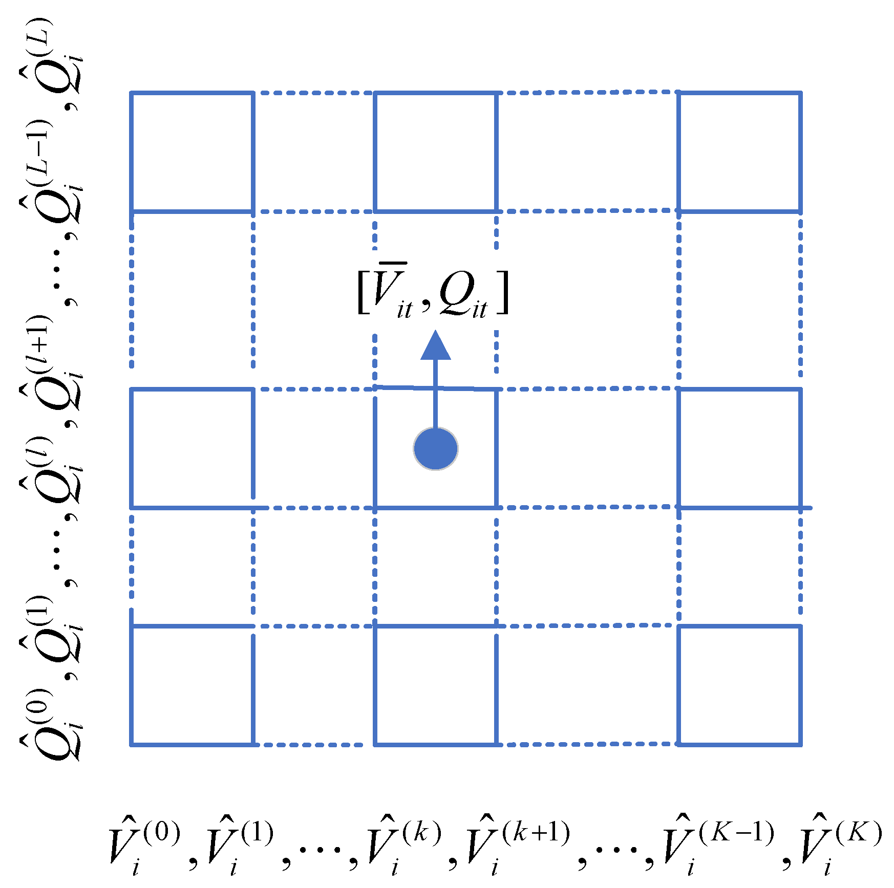
3.1. Spillage as a Nonlinear Function

The decision variables, q_it and h_it, only appear in constraints (4) and (7)–(9), where (7) and (8) are all the nonlinear constraints involved in the problem. From (4) and (8), we have

$$q_{it}\le \min [Q_{it},G_i^{\max }(h_{it})]$$

(11)

which, at the optimum, must be

$$q_{it}=\min [Q_{it},G_i^{\max }(h_{it})]$$

(12)

since this will violate no constraints but can help improve the objective by reducing the spillage and increasing the generating discharge that, according to (7), will increase the hydropower production.

The generating capacity (8) can be replaced with (12), which, along with (9), will help remove the decision variables (q_it and h_it) from the problem by replacing (4) and (7) with

$$\begin{array}{ll}sp{l}_{it}& =sp{l}_i({\overline{V}}_{it},Q_{it})\\ & =Q_{it}-\min \{Q_{it},G_i^{\max }[Z_i^{\mathrm{u}}({\overline{V}}_{it})-Z_i^{\mathrm{d}}(Q_{it})]\}\end{array}$$

(13)

$$\begin{array}{ll}{P}_{it}& =P_i({\overline{V}}_{it},Q_{it})\\ & =A_i\cdot \min \{Q_{it},G_i^{\max }[Z_i^{\mathrm{u}}({\overline{V}}_{it})-Z_i^{\mathrm{d}}(Q_{it})]\}\cdot [Z_i^{\mathrm{u}}({\overline{V}}_{it})-Z_i^{\mathrm{d}}(Q_{it})]\end{array}$$

(14)

which are nonlinear functions in an equivalent problem that has objective (1) subject to constraints: (2), (3), (5), (6), (10), (13), and (14).

3.2. SOS2 Formulation

The nonlinear functions (13) and (14) will be linearized with a special ordered set of type 2 (SOS2) formulation. A SOS2 is a set of consecutive variables in which no more than two adjacent members can be non-zero in a feasible solution. Knowing that a variable is part of a set and that it is ordered helps the branch and bound algorithm speed up the search procedure more intelligently.

As illustrated in Figure 1, the domain of storage (${\overline{V}}_{it}$) and outflow/release ($Q_{it}$) of a reservoir can be divided into rectangular grids by discrete values within their lower and upper bounds, denoted as:

$$V_i^{\mathrm{dead}}={\widehat{V}}_i^{(0)}<{\widehat{V}}_i^{(1)}<\cdots <{\widehat{V}}_i^{(k)}<\cdots <{\widehat{V}}_i^{(K)}=\underset{1\le t\le T}{\max }(\frac{V_{it}^{\max }+V_{i,t+1}^{\max }}{2})$$

(15)

$$Q_i^{\min }={\widehat{Q}}_i^{(0)}<{\widehat{Q}}_i^{(1)}<\cdots <{\widehat{Q}}_i^{(l)}<\cdots <{\widehat{Q}}_i^{(L)}=Q_i^{\max }$$

(16)

which determine a sample of spillages and storages at the corners of grids:

$$\left\{\begin{array}{l}s\widehat{p}{l}_i^{(k,l)}=sp{l}_{it}[{\widehat{V}}_i^{(k)},Q_i^{(l)}]\\ {\widehat{P}}_i^{(k,l)}=P_{it}[{\widehat{V}}_i^{(k)},Q_i^{(l)}]\end{array}\right.$$

(17)

Apparently, any point [${\overline{V}}_{it},Q_{it}$] can be covered by a convex combination of the grid corners:

$$\left\{\begin{array}{l}[{\overline{V}}_{it},Q_{it}]={\displaystyle \sum _{(k,l)}{\lambda }_{it}^{(k,l)}\cdot [{\widehat{V}}_i^{(k)},{\widehat{Q}}_i^{(l)}]}\\ {\displaystyle \sum _{(k,l)}{\lambda }_{it}^{(k,l)}}=1\end{array}\right.$$

(18)

where the spillage and hydropower output can be estimated as

$$sp{l}_{it}={\displaystyle \sum _{(k,l)}[{\lambda }_{it}^{(k,l)}\cdot s\widehat{p}{l}_i^{(k,l)}]}$$

(19)

$$P_{it}={\displaystyle \sum _{(k,l)}[{\lambda }_{it}^{(k,l)}\cdot {\widehat{P}}_i^{(k,l)}]}$$

(20)

in which ${\lambda }_{it}^{(k,l)}$ is the weight at the grid corner (k, l) for reservoir i. Particularly, enforcing that only the weights at the four corners of the grid where the point [${\overline{V}}_{it},Q_{it}$] is located can be non-zero will increase the linearization accuracy. To achieve this, let

$$a_{it}^{(k)}={\displaystyle \sum _{l=0}^L{\lambda }_{it}^{(k,l)}}$$

(21)

$$b_{it}^{(l)}={\displaystyle \sum _{k=0}^K{\lambda }_{it}^{(k,l)}}$$

(22)

And, as shown in

Table 1. Weights at corners of grids.

V	Q
	${\widehat{\mathit{Q}}}^{(0)}:{\mathit{x}}^{(0)}$	${\widehat{\mathit{Q}}}^{(1)}:{\mathit{x}}^{(1)}$	…	${\widehat{\mathit{Q}}}^{(\mathit{l})}:{\mathit{x}}^{(\mathit{l})}$	${\widehat{\mathit{Q}}}^{(\mathit{l}+1)}:{\mathit{x}}^{(\mathit{l}+1)}$	…	${\widehat{\mathit{Q}}}^{(\mathit{L})}:{\mathit{x}}^{(\mathit{L})}$
${\widehat{V}}^{(0)}:y^{(0)}$	${\lambda }^{(0,0)}$		…	${\lambda }^{(0,l)}$	${\lambda }^{(0,l+1)}$	…	${\lambda }^{(0,L)}$
${\widehat{V}}^{(1)}:y^{(1)}$	${\lambda }^{(1,0)}$		…	${\lambda }^{(1,l)}$	${\lambda }^{(1,l+1)}$	…	${\lambda }^{(1,L)}$
$⋮$	$⋮$	$⋮$	$\ddots$	$⋮$	$⋮$	$\ddots$	$⋮$
${\widehat{V}}^{(k)}:y^{(k)}$	${\lambda }^{(k,0)}$		…	${\lambda }^{(k,l)}$	${\lambda }^{(k,l+1)}$	…	${\lambda }^{(k,L)}$
${\widehat{V}}^{(k+1)}:y^{(k+1)}$	${\lambda }^{(k+1,0)}$		…	${\lambda }^{(k+1,l)}$	${\lambda }^{(0,l+1)}$	…	${\lambda }^{(k+1,L)}$
$⋮$	$⋮$	$⋮$	$\ddots$	$⋮$	$⋮$	$\ddots$	$⋮$
${\widehat{V}}^{(K)}:y^{(K)}$	${\lambda }^{(K,0)}$		…	${\lambda }^{(K,l)}$	${\lambda }^{(K,l+1)}$	…	${\lambda }^{(K,L)}$

, binary variables, $x_{it}^{(k)}$ and $y_{it}^{(l)}$, are introduced to decide whether the weights in the kth row and lth column can be greater than zero, respectively. If only two adjacent rows, rows k and k + 1 for instance, as well as two adjacent columns, columns l and l + 1 for instance, can have weights greater than zero, then it must be and can only be the four corners of the grid (k, l) that will have weights greater than zero and be active in estimating the functional values of spillage and hydropower output at any point located in this grid.

That only two adjacent rows can have non-zero weights can be ensured with

$$\left\{\begin{array}{l}{a}_{it}^{(k)}\le x_{it}^{(k)}\\ x_{it}^{(k)}\le x_{it}^{(k-1)}+x_{it}^{(k+1)}\le x_{it}^{(k)}+1\\ x_{it}^{(-1)}=0\\ x_{it}^{(K+1)}=0\\ {\displaystyle \sum _{k=0}^K{x}_{it}^{(k)}}=2\end{array}\right.$$

(23)

And similarly, for columns:

$$\left\{\begin{array}{l}{b}_{it}^{(l)}\le y_{it}^{(l)}\\ y_{it}^{(l)}\le y_{it}^{(l-1)}+y_{it}^{(l+1)}\le y_{it}^{(l)}+1\\ y_{it}^{(-1)}=0\\ y_{it}^{(L+1)}=0\\ {\displaystyle \sum _{l=0}^L{y}_{it}^{(l)}}=2\end{array}\right.$$

(24)

which ensures that when a binary variable ($y_{it}^{(l)}$) is equal to 1, then it must have one and only one of its adjacent binary variables [$y_{it}^{(l-1)}$ and $y_{it}^{(l+1)}$] equal to 1. The variables ($a_{it}^{(k)}$ and $b_{it}^{(l)}$) that satisfy constraints (23) and (24), respectively, are called the special ordered sets of type two (SOS2) and can be represented with:

$$SOS2\left(a_{it}^{(0)},a_{it}^{(1)},\cdots ,a_{it}^{(K)}\right)$$

(25)

$$SOS2\left(b_{it}^{(0)},b_{it}^{(1)},\cdots ,b_{it}^{(L)}\right)$$

(26)

which can be readily handled by a commercial LP solver.

Eventually, the original problem is equivalent to the one that has objective (1) subject to constraints: (2), (3), (5), (6), (10), (18)–(22), (25), and (26), which is a mixed integer linear Programming (MILP) that can be solved with an LP solver.

4. Case Studies

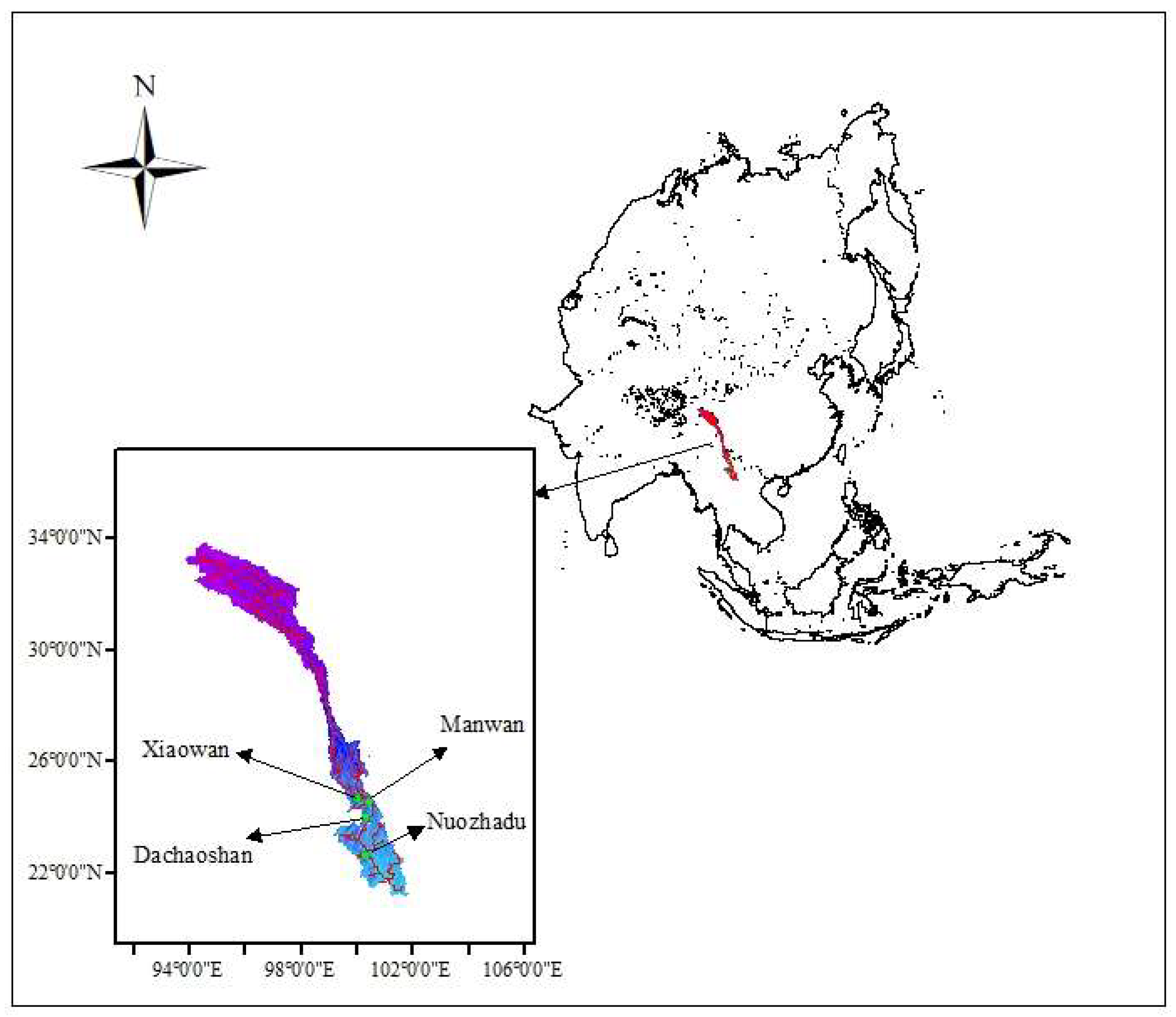
4.1. Engineering Background

The primary focus of this study revolves around the application of models and solution techniques specifically designed for the optimization of four cascaded reservoirs situated along the Lancang River, which, predominantly located within China, spans an extensive distance of 2161 km. The basin covers a vast area of 190,000 square kilometers, with China’s territory accounting for 167,400 square kilometers. The annual runoff depth in the basin is measured at 450.2 mm. The average yearly flow, an important reference point, is 2180 cubic meters per second. With the objective of this study in mind, four hydropower stations located within the basin are selected: Xiaowan, Manwan, Dachaoshan, and Nuozhadu. Each of them exhibits distinct regulation characteristics. Consequently, it becomes necessary to jointly schedule these four reservoirs to achieve the maximum benefit.

Table 2. Basic parameters of cascaded reservoirs.

Name	Installed Capacity (MW)	Storage Capacity (108 m3)	Dam Height (m)	Water Level (m)			Operability
				Flood	Normal	Dead
Xiaowan	4200	149.14	294.5	1232	1240	1166	Annual
Manwan	1670	5.02	132	994	994	988	Seasonal
Dachaoshan	1350	9.40	111	899	899	887	Seasonal
Nuozhadu	5850	126.70	261.5	804	812	765	Over-year

provides an overview of the four selected hydropower stations.

Figure 2 shows the location of the Lancang River basin in Asia, depicting the hydraulic connections of Xiaowan, Manwan, Dachaoshan, and Nuozhadu.

The Lancang River Basin is rich in water resources, where the hydropower stations usually have large reservoir capacity and good operability, which makes them have great research potential in controlling abandoned water. The four selected hydropower stations: Xiaowan, Manwan, Dachaoshan, and Nuozhadu are arranged in a certain hydrological order and height difference to form a cascade structure with different regulation ability: over-year regulation, annual regulation, and seasonal regulation, respectively.

The data in case studies are derived from inherent parameters and historical materials given by the hydropower stations. (Huaneng Lancang River Hydropower Inc., Yunnan Province, China. https://www.hnlcj.cn/, accessed on 20 August 2023).

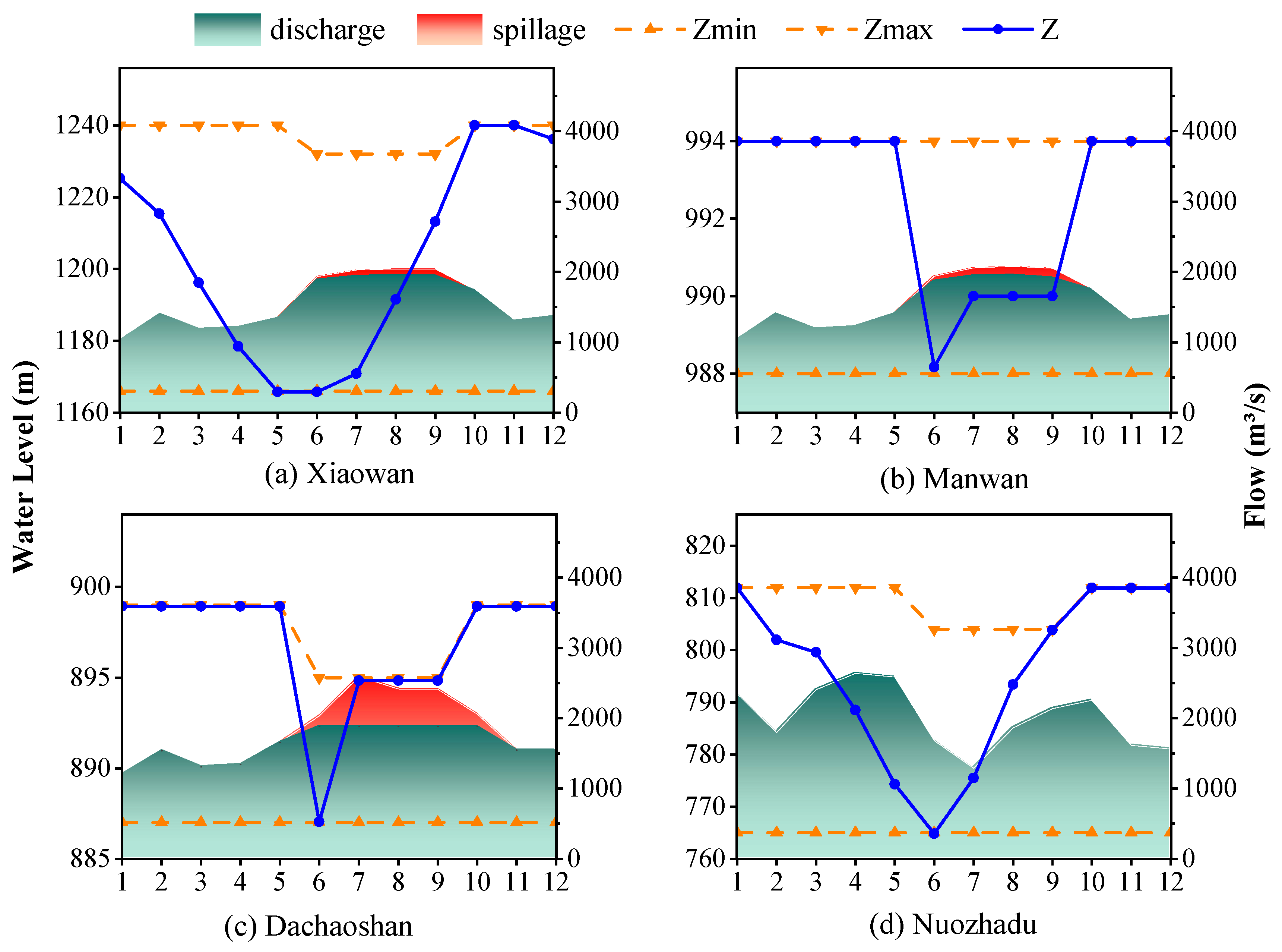
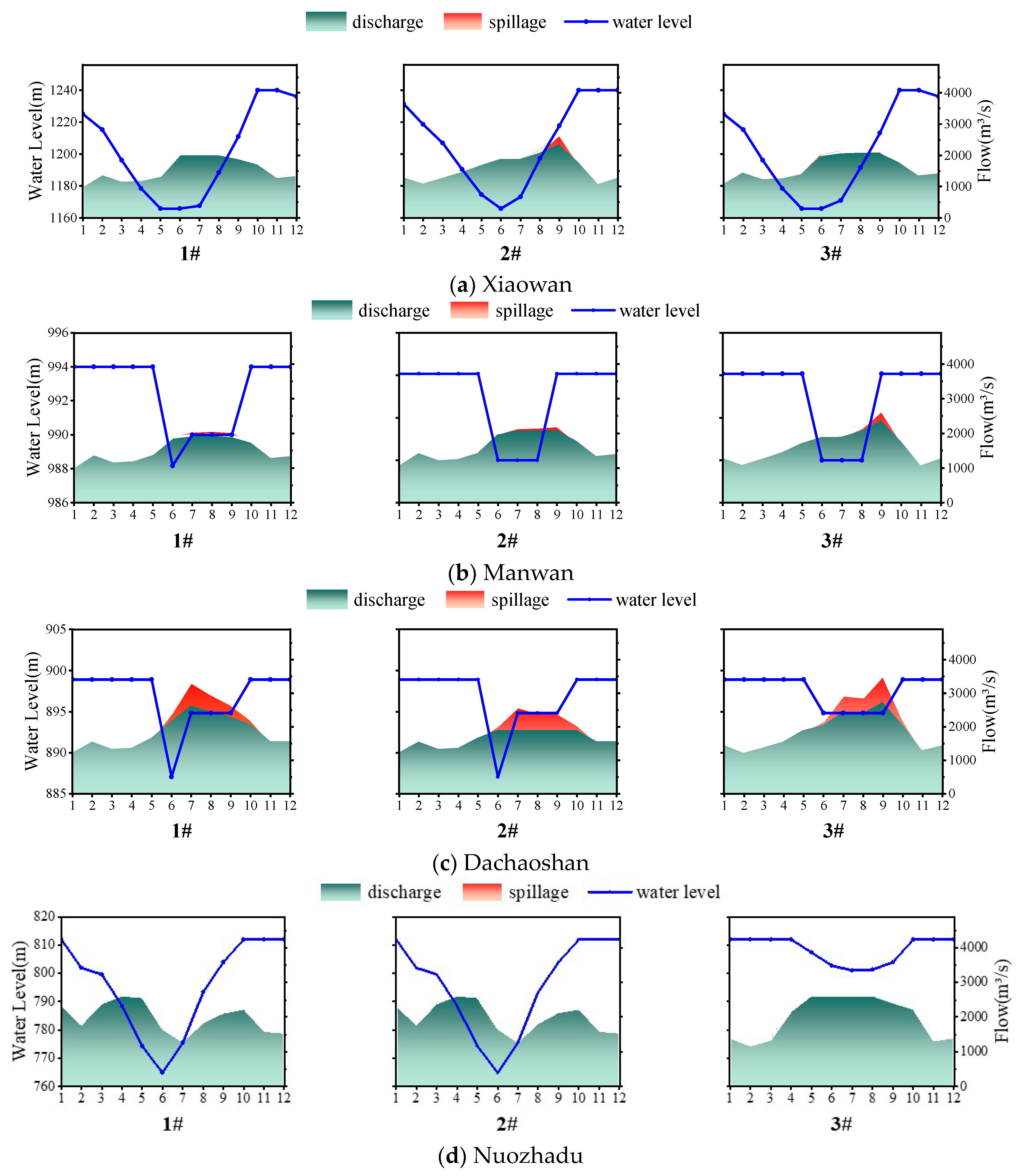
4.2. Detailed Results of Four Cascaded Hydropower Plants

The models and procedures were implemented in Python and executed on an Intel Core i7-8750H computer. Gurobi 9.5.2 was employed as the solver. This case occurs in a wet year (2020, with an average inflow of 1557.25 m³/s) and provides detailed results of the optimal scheduling process for the four cascaded hydropower reservoirs on the Lancang River, shown in Figure 3. Zmin means the lowest water level during the scheduling, which generally refers to the dead water level. Likewise, Zmax is the highest water level, which refers to the normal water lever in non-flood seasons and the flood-control water level during the flood seasons, respectively. Z denotes the water level for the current time period in the model. Despite lacking upstream reservoirs for assistance, Xiaowan, renowned for its robust regulating capacity, experiences a limited degree of spillage during the flood season, typically between June and September. Owing to its limited regulation capability, Manwan has spillages that occurred during the flood season. At all hydropower plants, the observed monthly water levels exhibit a consistent pattern characterized by increased water levels during dry seasons and a subsequent decrease during flood seasons. This pattern aims to minimize spillage and maximize hydroelectric generation, ensuring optimal utilization of water resources. During the flood months of July, August, and September, the Dachaoshan reservoir dedicates a portion of its storage capacity to fulfill the essential flood control requirements. This strategic allocation ensures that the reservoir can effectively manage and mitigate flood-related challenges during this specific period.

During the flood season, the Xiaowan and Manwan reservoirs still produce a small amount of spillage even when the water level does not reach its maximum capacity. This is because, although flood control requirements are met, power output limitations and reservoir scheduling strategies need to be considered. On the one hand, hydropower stations are subject to constraints imposed by generator capacity, preventing the complete utilization of the available flow for power generation, resulting in the generation of a small amount of spillage. On the other hand, hydropower stations generate spillage in the early stage so that they can avoid a large amount of spillage in the later period when the inflow is large.

Table 3. Summary of model results.

Station		Starting Conditions	Jan	Feb	Mar	Apr	May	Jun	Jul	Aug	Sept	Oct	Nov	Dec
Xiaowan	Local Inflow (m3/s)		433	394	434	780	1350	2098	2844	3147	3781	1747	1037	642
	Storage (mcm)	11,937.09	10,380.27	7761.05	5785.14	4642	4642	5073.75	7194.42	10,054.05	14,557	14,557	13,841.62	11,937.09
	Qspl (m3/s)		0	0	0	0	0	36.02	76.14	83.75	89.67	0	0	0
	Qhp (m3/s)		1033.63	1404.5	1196.31	1221.02	1350	1895.41	1949.70	1960	1954.08	1747	1313.00	1376.77
	Power (MW)		2160.69	2742.34	2137.16	2007.89	2133.77	3018.06	3342.26	3739.61	4168.22	3939.98	2950.53	2999.469
	Energy (GWh)		1607.55	1908.67	1590.05	1445.68	1587.53	2173.01	2486.64	2782.27	3001.12	2931.34	2124.381	2231.61
Manwan	Local Inflow (m3/s)		1038.63	1408.5	1201.31	1229.02	1364	1953.43	2055.84	2076.75	2083.75	1765	1324.00	1383.77
	Storage (mcm)	372	372	372	372	372	249	284.1	284.1	284.1	372	372	372	372
	Qspl (m3/s)		0	0	0	0	0	56.40	102.61	110.94	120.02	0	0	0
	Qhp (m3/s)		1038.63	1408.5	1201.31	1229.02	1411.45	1883.48	1953.23	1965.81	1929.82	1765	1324	1383.77
	Power (MW)		821.59	1103.93	945.78	966.94	1073.60	1385.82	1448.42	1457.18	1465.22	1376.05	1039.43	1085.05
	Energy (GWh)		611.27	768.34	703.66	696.19	798.76	997.79	1077.62	1084.14	1054.96	1023.78	748.39	807.28
Dachaoshan	Local Inflow (m3/s)		1200.63	1537.5	1309.31	1338.02	1547.45	2099.87	2591.84	2416.75	2448.84	2060	1546	1540.77
	Storage (mcm)	740	740	740	740	740	465	637	637	637	740	740	740	740
	Qspl (m3/s)		0	0	0	0	0	150.53	708.84	533.75	526.1	177	0	0
	Qhp (m3/s)		1200.63	1537.5	1309.31	1338.02	1653.55	1883	1883	1883	1883	1883	1546	1540.77
	Power (MW)		859.72	1076.78	929.52	947.95	1073.61	1169.65	1195.14	1206.40	1241.09	1294.89	1082.35	1078.92
	Energy (GWh)		639.63	749.44	691.57	682.53	798.76	842.15	889.19	897.56	893.59	963.40	779.29	802.72
Nuozhadu	Local Inflow (m3/s)		1200.63	1537.5	1323.31	1447.02	1895.549	2461.53	2852.84	2957.75	3069.1	2254	1614	1563.77
	Storage (mcm)	21,749	18,776.28	18,109.63	15,296.7	12,203.22	10,414	12,441.58	16,500.31	19,337	21,749	21,749	21,749	21,749
	Qspl (m3/s)		0	0	0	0	0	0	0	0	0	0	0	0
	Qhp (m3/s)		2347.51	1794.7	2408.55	2640.5	2585.83	1679.28	1286.97	1863.35	2138.54	2254	1614	1563.77
	Power (MW)		4257.04	3175.99	4086.57	4176.26	3818.06	2525.50	2113.22	3262.11	3906.89	4187.95	3026.73	2935.59
	Energy (GWh)		3167.24	2210.49	3040.41	3006.91	2840.64	1818.36	1572.23	2427.01	2812.96	3115.84	2179.24	2184.08

provides a comprehensive summary of the entire model results, encompassing the inflow, reservoir capacity, spillage, power generation flow rate, power generation, and energy for the four power stations over 12 time steps.

4.3. Solution Efficiency of SOS2 Modeling

Table 4. Model Results under Different Grid Densities.

	4 × 4	8 × 8	15 × 15	20 × 20	25 × 25
Spillage (m3/s)	30,731.2	13,799.8	2431.4	2128.3	1951.4
F (MW)	5,511,737.2	7,067,768.6	8,042,369.1	8,097,267.3	8,093,758.3
P (MW)	72,789,359.6	90,731,379.7	103,268,755.2	103,975,851.6	104,052,755.0
Obj	25,146,663.1	6,641,342.9	−5,714,286.2	−6,072,947.9	−6,246,391.5
Number of variables	1495	4183	12,583	21,181	32,462
CPU time (s)	0.14	0.68	4.70	10.00	31.59

summarizes model results under different gridding resolutions for five cases. As the grid density increases, all components of the objectives become superior, indicating that higher grid density leads to a better scheduling solution. However, an increase in grid density leads to a significant increase in the number of variables, which explains the growth of CPU time.

The term “Obj” in Table 4 refers to the optimal value of Equation (1):

$$\min {\mathrm{W}}_1\cdot {\displaystyle \sum _{i=1}^N[{\eta }_i^{QP}{\displaystyle \sum _{t=0}^{T-1}sp{l}_{it}}}]-{\mathrm{W}}_2\cdot F-{\mathrm{W}}_3\cdot {\displaystyle \sum _{i=1}^N{\displaystyle \sum _{t=0}^{T-1}{P}_{it}}}$$

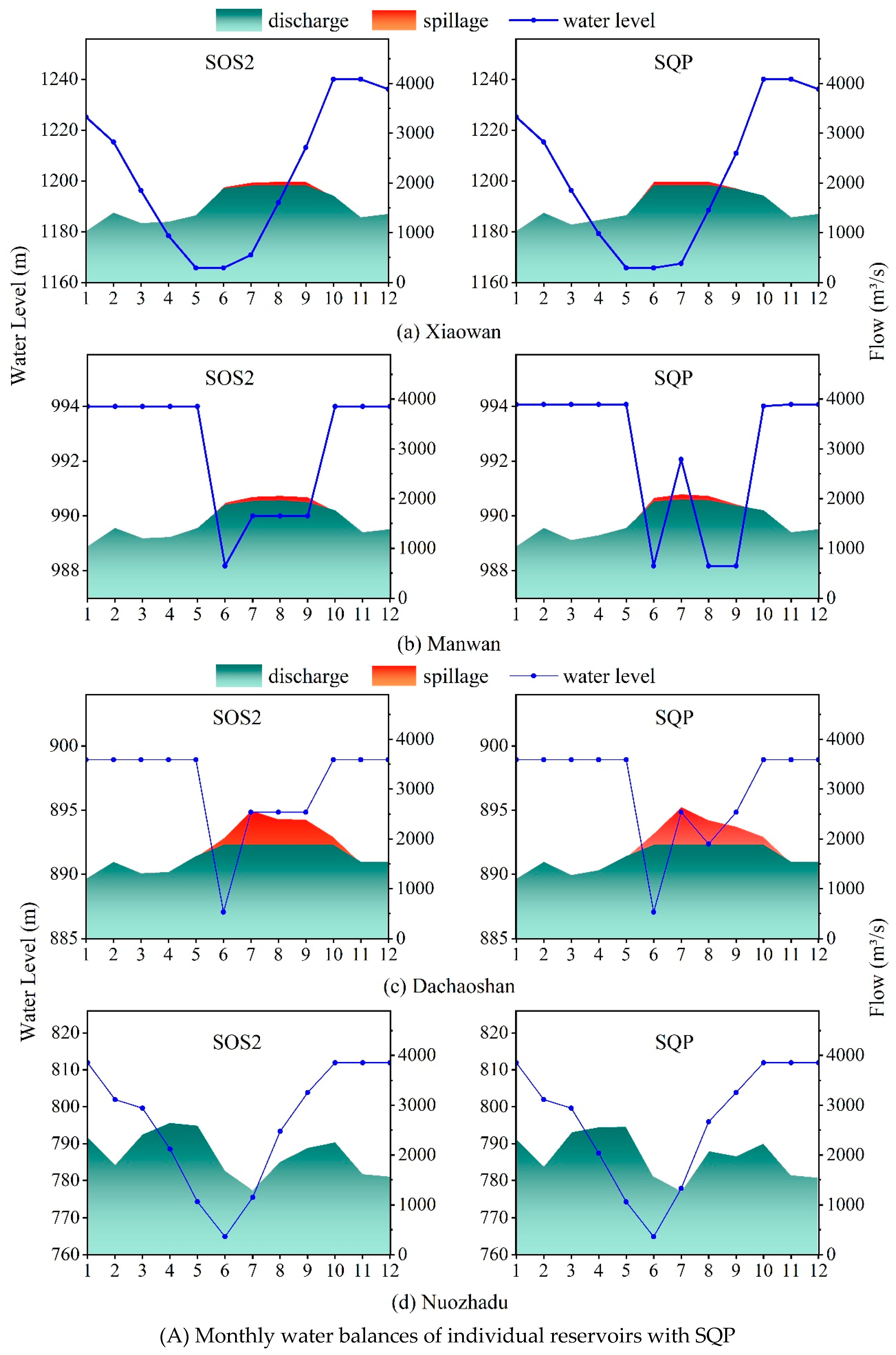
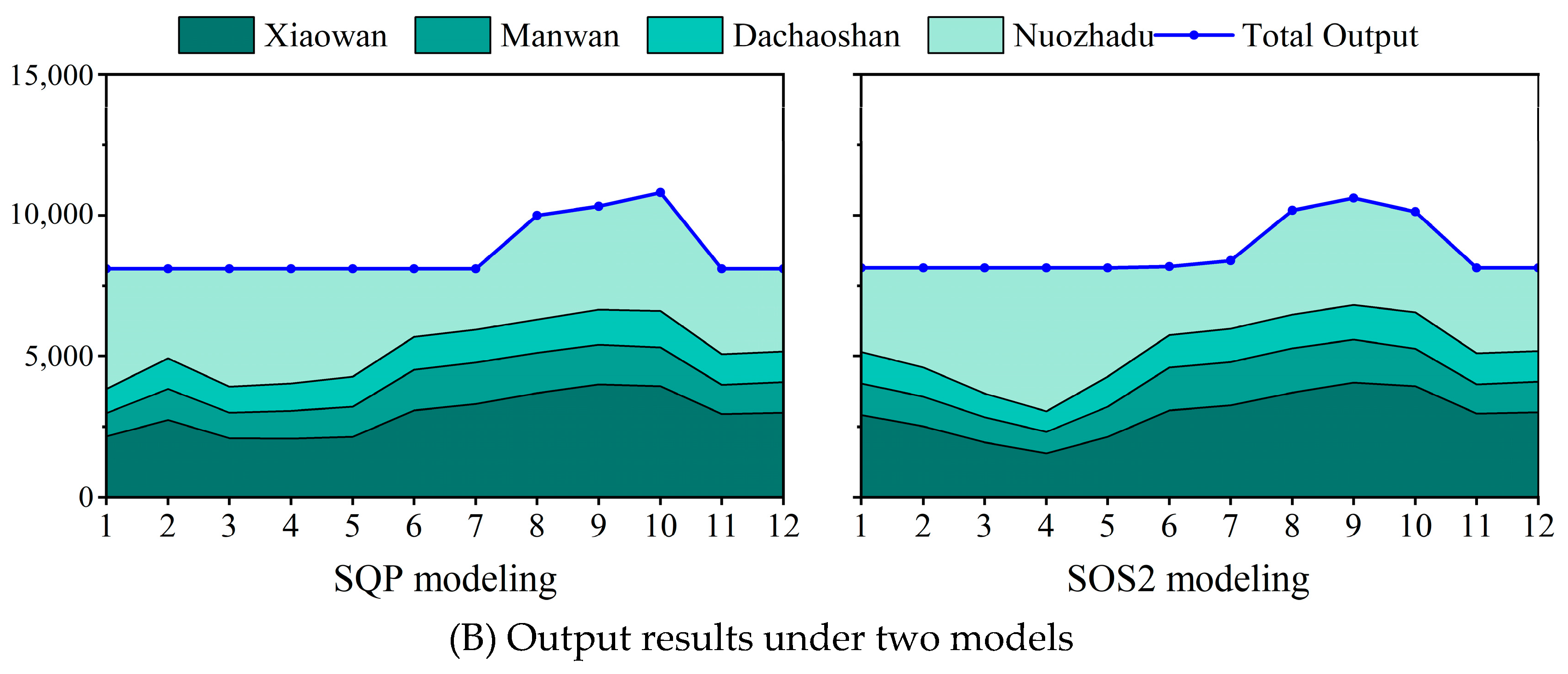
4.4. Comparisons with SQP

This work comprehensively compared the SOS2 modeling and the SQP (Successive Quadratic Programming) method to validate the superiority of the proposed model.

Table 5. Model Results under Different Grid Densities.

	∑Spillage (m3/s)	F (GW)	∑P (GW)	Obj (MW)	Number of Variables	CPU Time (s)
SOS2	2734.58	8.09	104.05	−6246.39	32,462	31.59
SQP	2750.66	8.04	104.00	−6074.57	725	100.19
	0.58% ↓	0.62% ↑	0.05 ↑	2.83% ↓	-	0.68% ↓

shows detailed comparisons of the results of the two methods for the same scheduling problem. ↓ means that the proportion by which the SOS2 model reduces the specific target value compared to the SQP model within that target value. ↑ means that the proportion by which the SOS2 model enhances the specific target value relative to the SQP model in that target value.

Both the SQP and SOS2 belong to mathematical optimization methods, which are suitable for solving optimization problems with constraints and continuous nonlinear objective functions. The comparison between the two makes more sense. The theory and implementation of SQP are relatively mature, and have a wide range of applications in long-term scheduling problems. In contrast, the performance of the SOS2 model can be evaluated, which can not only verify the experimental results, but also illuminate its advantages and limitations.

Overall, the SOS2 model outperforms the SQP model regarding both solution efficiency and objective benefits. Specifically, the SOS2 modeling reduces water spillage by 0.58%, increases firm output by 0.62%, and improves power generation by 0.05% compared to the SQP model. Additionally, the SOS2 model achieves these improvements while reducing the CPU time by about 67 s.

Figure 4 displays the monthly outcomes of the two models, showcasing a comparison of water balances and hydropower outputs. Notably, Xiaowan and Dachaoshan, renowned for their superior regulation capacities within the cascade system, exhibit a similar water balance pattern across both models. Conversely, Manwan and Dachaoshan in the SQP model show a sudden surge in water levels during July. However, the monthly hydropower outputs remain relatively consistent and closely aligned between the two models.

4.5. Impacts on Results by Prioritizing the Objectives in Different Ways

To illustrate the impact of different allocations of objectives,

Table 6. Results when assigning different priorities to objectives.

Experiments	Weights			Spillage	Firm Output	Total Output
	W1	W2	W3	(hm3)	(MW)	(GW)
1#	1000	1	0.001	6318.709	7914.266	104.053
2#	0.001	1000	1	6355.715	8138.426	104.237
3#	0.001	1	1000	6601.307	6917.175	107.122

provides the results of the weights W1, W2, and W3 under different priority orders, which are assigned to spillage, firm output, and total output, respectively. The objective function minimizes spillage while maximizing firm hydropower and power output. It is evident that increasing the priority weight will improve the corresponding objective, while the remaining two objectives will decrease sequentially.

Also, as shown in Figure 5, the obtained results indicate that assigning priority to minimizing spillage and achieving firm hydropower output yields more closely aligned outcomes than prioritizing energy production. This finding suggests a certain degree of consistency between minimizing spillage and maximizing firm hydropower output. On the other hand, maximizing hydropower production tends to maintain higher water levels in downstream reservoirs such as Dachaoshan and Manwan. The findings of this analysis can provide valuable insights for companies to balance and evaluate various scheduling options during critical periods effectively. By considering the trade-offs between minimizing spillage, maximizing firm hydropower output, and optimizing energy production, companies can make informed decisions to optimize their operational strategies and achieve a balanced approach to managing water resources and power generation.

5. Conclusions

This work utilizes SOS2 modeling to address a monthly hydropower scheduling problem. By employing interpolation within a gridding domain defined by storage and outflow, the hydropower output and spillage become controllable and linearized, enabling efficient optimization of the scheduling process. The model and method were applied to four cascaded hydropower plants on the Lancang River, and the case studies suggest the following.

The presented SOS2 modeling approach proves to be highly applicable and yields reliable results for the monthly scheduling of cascaded reservoirs.

Higher grid density improves scheduling solutions. The proposed SOS2 model outperformed the SQP model in solution efficiency and objective benefits, reducing CPU time by approximately 67 s. However, practical application in large-scale hydropower systems may be limited by increasing computation time with more grid points, requiring more efficient computational methods to improve feasibility.

The model proposed in this work still has significant room for further improvement.

Consideration of uncertainty: Many factors affecting reservoir operation are uncertain, such as inflow, electricity demand, and future climate conditions. The introduction of uncertainty modeling and robust optimization techniques can improve the resilience and reliability of the system and make it more adaptable to changes in the real world.

Consideration of practical constraints: The actual hydropower system usually faces various operational constraints, environmental regulations, and social problems. Future research should consider these factors to ensure that the analysis model is still practical and applicable in practical applications.

Certainly, due to the limitations of the incomplete consideration during the modeling process, the proposed model in this study possesses certain limitations.

Linearization error: The use of SOS2 for nonlinear linearization may introduce approximation errors, resulting in a suboptimal solution relative to the solution to the original nonlinear problem. Researchers should carefully evaluate the trade-off between linearization error and computational efficiency.

Using months as the time steps may not be optimal for minimizing reservoir spills, primarily attributable to the relatively flat shape of monthly inflow hydrographs in comparison to those derived from weekly time steps. Researchers discovered that the elevated spills observed in weekly simulations as opposed to monthly simulations can be solely attributed to the distinct hydrograph shapes between the two time step resolutions [32]. In future work, further reductions in the time step will be explored.

References

1. Wang, H.; Wang, X.; Lei, X.; Liao, W.; Wang, C.; Wang, J. The development and prospect of key techniques in the cascade reservoir operation. J. Hydraul. Eng. 2019, 50, 25–37. [Google Scholar]
2. Ming, B.; Huang, Q.; Wang, Y.; Wei, J.; Tian, T. Search space reduction method and its application to hydroelectric operation of multi-reservoir systems. J. Hydroelectr. Eng. 2015, 34, 51–59. [Google Scholar]
3. Zheng, H.; Feng, S.; Chen, C.; Wang, J. A new three-triangle based method to linearly concave hydropower output in long-term reservoir operation. Energy 2022, 250, 123784. [Google Scholar] [CrossRef]
4. Zhuang-zhi, G.U.O.; Jie-kang, W.U.; Fan-nie, K.; Yu-nan, Z.H.U. Long-Term Optimization Scheduling Based on Maximal Storage Energy Exploitation of Cascaded Hydro-plant Reservoirs. Proc. Chin. Soc. Electr. Eng. 2010, 30, 20–26. [Google Scholar]
5. Little, J.D.C. The Use of Storage Water in a Hydroelectric System. J. Oper. Res. Soc. Am. 1955, 3, 187–197. [Google Scholar] [CrossRef]
6. Ahmed, J.A.; Sarma, A.K. Genetic Algorithm for Optimal Operating Policy of a Multipurpose Reservoir. Water Resour. Manag. 2005, 19, 145–161. [Google Scholar] [CrossRef]
7. Guo, X.; Qin, T.; Lei, X.; Jiang, Y.; Wang, H. Advances in derivation method for multi-reservoir joint operation policy. J. Hydroelectr. Eng. 2016, 35, 19–27. [Google Scholar]
8. Denham, W. Differential dynamic programming. IEEE Trans. Autom. Control 1971, 16, 389–390. [Google Scholar] [CrossRef]
9. Shi, Y.; Peng, Y.; Xu, W. Optimal operation model of cascade reservoirs based on grey discrete differential dynamic programming. J. Hydroelectr. Eng. 2016, 35, 35–44. [Google Scholar]
10. Liu, S.; Luo, J.; Chen, H.; Wang, Y.; Li, X.; Zhang, J.; Wang, J. Third-Monthly Hydropower Scheduling of Cascaded Reservoirs Using Successive Quadratic Programming in Trust Corridor. Water 2023, 15, 716. [Google Scholar] [CrossRef]
11. Jothiprakash, V.; Arunkumar, R. Optimization of Hydropower Reservoir Using Evolutionary Algorithms Coupled with Chaos. Water Resour. Manag. 2013, 27, 1963–1979. [Google Scholar] [CrossRef]
12. Wardlaw, R.; Sharif, M. Evaluation of Genetic Algorithms for Optimal Reservoir System Operation. J. Water Resour. Plan. Manag. 1999, 125, 25–33. [Google Scholar] [CrossRef]
13. Ma, J.; Teng, G. Study on the feature construction method based on genetic programming. J. Agric. Univ. Hebei 2018, 41, 130–136. [Google Scholar]
14. Wei, Z.Y.Z.; Zhiwu, L.; Pan, L.; Mengjie, L. Deep learning model guided by physical mechanism for reservoir operation. J. Hydroelectr. Eng. 2023, 42, 13–25. [Google Scholar] [CrossRef]
15. Zhou, J.; Peng, T.; Zhang, C.; Sun, N. Data Pre-Analysis and Ensemble of Various Artificial Neural Networks for Monthly Streamflow Forecasting. Water 2018, 10, 628. [Google Scholar] [CrossRef]
16. Baltar, A.M.; Fontane, D.G. Use of Multiobjective Particle Swarm Optimization in Water Resources Management. J. Water Resour. Plan. Manag. 2008, 134, 257–265. [Google Scholar] [CrossRef]
17. Zhang, X.; Yu, X.; Qin, H. Optimal operation of multi-reservoir hydropower systems using enhanced comprehensive learning particle swarm optimization. J. Hydro-Environ. Res. 2016, 10, 50–63. [Google Scholar] [CrossRef]
18. Diao, Y.; Ma, H.; Wang, H.; Wang, J.; Li, S.; Li, X.; Pan, J.; Qiu, Q. Optimal Flood-Control Operation of Cascade Reservoirs Using an Improved Particle Swarm Optimization Algorithm. Water 2022, 14, 1239. [Google Scholar] [CrossRef]
19. Dorigo, M.; Maniezzo, V.; Colorni, A. Ant system: Optimization by a colony of cooperating agents. IEEE Trans. Syst. Man Cybern. Part B 1996, 26, 29–41. [Google Scholar] [CrossRef]
20. Wang, C.; Zhou, J.; Lu, P.; Yuan, L. Long-term scheduling of large cascade hydropower stations in Jinsha River, China. Energy Convers. Manag. 2015, 90, 476–487. [Google Scholar] [CrossRef]
21. Zhou, B.; Feng, S.; Xu, Z.; Jiang, Y.; Wang, Y.; Chen, K.; Wang, J. A Monthly Hydropower Scheduling Model of Cascaded Reservoirs with the Zoutendijk Method. Water 2022, 14, 3978. [Google Scholar] [CrossRef]
22. Feng, S.Z.; Zheng, H.; Qiao, Y.F.; Yang, Z.T.; Wang, J.W.; Liu, S.Q. Weekly hydropower scheduling of cascaded reservoirs with hourly power and capacity balances. Appl. Energy 2022, 311, 118620. [Google Scholar] [CrossRef]
23. Wang, C.; Guo, S.; Liu, P.; Zhou, F.; Xiong, L. Risk criteria and comprehensive evaluation model for the operation of Three Gorges reservoir under dynamic flood limit water level. Adv. Water Sci. 2004, 15, 376–381. [Google Scholar]
24. Ai, X.; Fan, W. On Reservoir Ecological Operation Model. Resour. Environ. Yangtze Basin 2008, 17, 451–455. [Google Scholar]
25. Zhang, W.; Wang, X.; Lei, X.; Liu, P.; Wang, H. Adaptive reservoir operating rules based on the Dempster-Shafer evidence theory. Adv. Water Sci. 2018, 29, 685–695. [Google Scholar]
26. Zhong, J.; Dong, Z.; Yao, H.; Ni, X.; Chen, M.; Jia, W.; Ye, H. Multi-objective operation rules for cascade reservoirs. Case study of Xiluodu-Xiangjiaba cascade. J. Hydroelectr. Eng. 2021, 40, 46–54. [Google Scholar]
27. Chen, C.; Kang, C.; Wang, J. Stochastic Linear Programming for Reservoir Operation with Constraints on Reliability and Vulnerability. Water 2018, 10, 175. [Google Scholar] [CrossRef]
28. Beale, E.; Tomlin, J. Special facilities in a general mathematical programming system for nonconvex problems using ordered sets of variables. Oper. Res. 1969, 69, 447–454. [Google Scholar]
29. Beale, E. Branch and Bound Methods for Mathematical Programming Systems. Ann. Discret. Math. 1979, 5, 201–219. [Google Scholar] [CrossRef]
30. Kang, C.; Guo, M.; Wang, J. Short-Term Hydrothermal Scheduling Using a Two-Stage Linear Programming with Special Ordered Sets Method. Water Resour. Manag. 2017, 31, 3329–3341. [Google Scholar] [CrossRef]
31. Yu, H.J.X.; Shen, J.J.; Cheng, C.T.; Lu, J.; Cai, H.X. Multi-Objective Optimal Long-Term Operation of Cascade Hydropower for Multi-Market Portfolio and Energy Stored at End of Year. Energies 2023, 16, 604. [Google Scholar] [CrossRef]
32. Ilich, N. WEB.BM-a web-based river basin management model with multiple time-step optimization and the SSARR channel routing options. Hydrol. Sci. J. J. DES Sci. Hydrol. 2022, 67, 175–190. [Google Scholar] [CrossRef]
Figure 1. Gridding for piecewise linearization.
Water 15 03128 g001
Figure 2. The location of the Lancang River basin in Asia, depicting the hydraulic connections of Xiaowan, Manwan, Dachaoshan, and Nuozhadu.
Water 15 03128 g002
Figure 3. Monthly hydropower schedules over a year.
Water 15 03128 g003
Figure 4. Comparison of scheduling results between two models.
Water 15 03128 g004aWater 15 03128 g004b
Figure 5. Scheduling results under different weight values.
Water 15 03128 g005