
Predicting Daily Streamflow in a Cold Climate Using a Novel Data Mining Technique: Radial M5 Model Tree
by
 , , and
Ozgur Kisi
1,2,* ,
,
Salim Heddam
3 ,
,
Behrooz Keshtegar
4, 
Jamshid Piri
5 and
Rana Muhammad Adnan
6,* 1
Department of Civil Engineering, University of Applied Sciences, 23562 Lübeck, Germany
2
Civil Engineering Department, Ilia State University, 0162 Tbilisi, Georgia
3
Agronomy Department, Faculty of Science, Hydraulics Division University, 20 Août 1955, Route El Hadaik, BP 26, Skikda 21024, Algeria
4
Department of Civil Engineering, Faculty of Engineering, University of Zabol, Zabol 9861335856, Iran
5
Department of Water Engineering, Faculty of Water and Soil, University of Zabol, Zabol 9861335856, Iran
6
State Key Laboratory of Hydrology-Water Resources and Hydraulic Engineering, Hohai University, Nanjing 210098, China
*
Authors to whom correspondence should be addressed.
Water 2022, 14(9), 1449; https://doi.org/10.3390/w14091449
Submission received: 31 March 2022
/
Revised: 23 April 2022
/
Accepted: 27 April 2022
/
Published: 1 May 2022
(This article belongs to the Special Issue River Flow in Cold Climate Environments)
Abstract
:In this study, the viability of radial M5 model tree (RM5Tree) is investigated in prediction and estimation of daily streamflow in a cold climate. The RM5Tree model is compared with the M5 model tree (M5Tree), artificial neural networks (ANN), radial basis function neural networks (RBFNN), and multivariate adaptive regression spline (MARS) using data of two stations from Sweden. The accuracy of the methods is assessed based on root mean square errors (RMSE), mean absolute errors (MAE), mean absolute percentage errors (MAPE), and Nash Sutcliffe Efficiency (NSE) and the methods are graphically compared using time variation and scatter graphs. The benchmark results show that the RM5Tree offers better accuracy in predicting daily streamflow compared to other four models by respectively improving the accuracy of M5Tree with respect to RMSE, MAE, MAPE, and NSE by 26.5, 17.9, 5.9, and 10.9%. The RM5Tree also acts better than the M5Tree, ANN, RBFNN, and MARS in estimating streamflow of downstream station using only upstream data.
1. Introduction
Streamflow forecasting helps in providing reliable and useful information for water management, flood warning, and reservoir flood management with respect to near, medium, and long-term considerations [1,2,3], and it has a role to play in the acquisition of the observed and continuous data required to address our knowledge on water resources planning [4]. However, the uncertainty still exists and the need for introducing new and robust forecasting strategies remains a challenge [5]. More precisely, an accurate streamflow forecasting can be integrated into global water, agricultural, and industry program, and a continuous progress in predicting and forecasting streamflow at several time steps has attracted a great deal of attention over the world, and the use of measured and available weather and hydrological variables, i.e., precipitation (P), air temperature (Ta), evapotranspiration (EP) among others, has considerably advanced in recent years [6]. In a recently conducted investigation for the Colorado River basin in the United States (USA), Towler et al. [7] demonstrated that streamflow is highly sensitive to the variation of Ta and P. Several kinds of approaches can be used for accurately predicting streamflow, ranging from physically based, conceptual, statistical, and stochastic, to data-driven artificial intelligence (AI) models [8,9]. During the last few years, the application of AI models for streamflow has significantly increased and there has been an explosion in the number of published papers, showing a variety of proposed modelling approaches from single to hybrid models with and without preprocessing schemas, and more precisely deep leaning paradigm is beginning to have an impact on the overall streamflow forecasting accuracies.
Among the famous deep learning algorithm, the long-short term memory (LSTM) artificial neural network has attracted the interest of researchers. For example, Hunt et al. [6] used the LSTM artificial neural network for predicting streamflow at several rivers across various climatic regions of the western United States (USA), and a hybrid model combining the Global Flood Awareness System ERA5 and GloFAS-ERA5 reanalysis and in situ measured historical streamflow was proposed. The proposed hybrid model was applied to predict streamflow up to ten days in advance, and it was found that the LSTM performed the best with a Nash–Sutcliffe efficiency (NSE) exceeding ≈0.900 during the testing phase. Wegayehu and Muluneh [10] tested the performances of three deep learning models namely, stacked long short-term memory (S-LSTM), bidirectional long short-term memory (Bi-LSTM), and gated recurrent unit (GRU) with the multilayer perceptron neural network (MLPNN) for one-step daily streamflow forecasting in the Awash and Abay rivers located in Ethiopia. By testing several input combination of lagged time series of streamflow data, it was found that, at short-term streamflow forecasting the MLPNN and GRU surpassed the S-LSTM and Bi-LSTM. Cho and Kim [11] compared three models namely, weather research and forecasting hydrological modeling system (WRF-Hydro), LSTM network, and coupled WRF-Hydro-LSTM for predicting streamflow in south Korea. While the LSTM was used for predicting the residual error of the WRF-Hydro, it was found that the combined WRF-Hydro-LSTM provided more accurate results exhibiting NSE value greater than ≈0.95 compared to the value of ≈0.72 obtained using the WRF-Hydro. Essam et al. [12] applied three machine learning models namely, the LSTM, the support vector regression (SVR), and the MLPNN for predicting streamflow using data collected at 11 rivers in Peninsular Malaysia. It was found that the MLPNN with three-lag times of streamflow as input variables exhibited the best accuracy with the high R2 value of approximately ≈0.900 in some rivers, while it failed completely for providing acceptable accuracies in other rivers. Liu et al. [13] compared convolutional neural networks (CNN), directed graph deep neural network (DGDNN), LSTM and GRU models for multi-steps ahead forecasting of daily streamflow up to seven days in advance. It was found that the DGDNN was slightly more accurate compared to the other models with NSE values ranging from ≈0.928 to ≈0.970. Afan et al. [14] compared two different deep learning methods, deep learning-based linear selection (LDL) and deep learning-based stratified selection (SDL) for forecasting monthly streamflow in the Tigris River, Irak. It was found that the SDL improves the accuracy of the LDL by about 7.96% to 94.6%.
Hybrid and optimized data-driven models using metaheuristics algorithms were among the most well-known reported models for streamflow forecasting. Danandeh Mehr et al. [15] compared genetic programming (GP), seasonal autoregressive integrated moving average (SARIMA), and hybrid GP-SARIMA for forecasting daily, weekly, and monthly streamflow in the headwaters of the Oulujoki River, Finland. Using the average mutual information (AMI) algorithm for better selection of time lagged input variable, the authors reported that GP and SARIMA were relatively equal at daily time scale exhibiting the same forecasting accuracy with NSE values ranging from ≈0.996 to ≈0.997 and root mean square error (RMSE) values ranging from ≈0.155 to ≈0.188, while the models were failed to accurately predict weekly streamflow data. Hassan and Khan [16] combined P, Ta, and streamflow data measured at several time lags for better streamflow forecasting, and they compared Bayesian regularization neural networks (BRNN), random forest regression (RFR), and gradient boosting machine (GBM) for predicting streamflow at the Chitral River, Pakistan. The significant finding for the above reported study is that the authors have demonstrated that hybrid models based on BRNN combined with RFR and GBM, i.e., RFR- BRNN and GBM- BRNN were the most accurate compared to the single models, and the use of P coupled with Ta was more suitable for obtaining peak streamflow forecasting. Samantaray et al. [17] proposed an improved hybrid model based on support vector regression (SVR) hybridized using Salp swarm algorithm (SVR-SSA) for forecasting monthly streamflow in Baitarani river basin, Odisha, India. The authors used several input variables namely, P, Ta, relative humidity (H %), and river stage (RS). The performances of the SVR-SSA were compared to those of the MLPNN and the standalone SVR showing its superiority with R2 and RMSE of ≈0.977 and ≈2.72 compared to the values of ≈0.925 and ≈15.77 obtained using the SVR, and the values of ≈0.905 and ≈29.001 obtained using the MLPNN. Zhou et al. [18] have introduced a new modelling framework for streamflow prediction based on the combination of the arbitrary polynomial chaos expansion (aPCE) method and four data-driven models namely, the SVR, MLPNN, RFR, and k-nearest neighbors (KNN) algorithms incorporated into the fully distributed, physically based hydrologic modelling system (MIKE SHE). Based on the RMSE, MAE, and R2 values, it was found that the hybrid models outperformed the standalone MIKE SHE model. Nguyen et al. [19] have developed a hybrid model called GA-BART, which combines the genetic algorithm (GA) with the Bayesian additive regression tree (BART) for hourly streamflow forecasting. The performances of the GA-BART were compared to those of GA-SVR and multiple linear regression (MLR) models. It was found that the performances of all models significantly decreased by the increase of the forecasting horizon from 1 h to 6 h in advance and in overall, the GA-BART was more accurate exhibiting NSE values ranging from ≈0.47 to ≈0.96.
In a recently published paper, Khosravi et al. [20] used Bat metaheuristics algorithm for optimizing four data driven models namely, convolutional neural network (Bat-CNN), MLPNN (Bat-MLPNN), adaptive neuro-fuzzy inference system (Bat-ANFIS), support vector regression (Bat-SVR), and random forest regression (Bat-RFR). The developed hybrid models, i.e., Bat-CNN, Bat-MLPNN, Bat-RFR, Bat-SVR, and Bat-ANFIS were applied and compared for predicting daily streamflow in the Korkorsar catchment in northern Iran. According to the obtained results, the authors reported that: (i) rainfall at time t (Rt) was the most significant input variables, (ii) combining the (Rt), (Rt−1) and the streamflow (Qt) leads to the best forecasting accuracy, and (iii) the Bat-CNN was the most accurate model exhibiting high forecasting accuracy with correlation coefficient (R) higher than ≈0.95. The R values obtained using the ANFIS-BAT and SVR-BAT were ranged from ≈0.90 to ≈0.95, while the R values obtained using the RFR-BAT and MLPNN-BAT were ranged between ≈0.80 and ≈0.90, respectively. Extreme learning machine (ELM) was also reported as a powerful tool for streamflow forecasting. For example, Feng et al. [21] combined the ELM and the parallel cooperation search algorithm (PCSA) algorithm for providing a hybrid model called ELM-PCSA. The performances of the proposed ELM-PCSA were compared to those of ELM, ELM optimized genetic algorithm (ELM-GA), ELM optimized particle swarm optimization (ELM-PSO), ELM optimized differential evolution (ELM-DE), ELM optimized gravitational search algorithm (ELM-GSA), and ELM optimized cooperation search algorithm (CSA), respectively. By testing all proposed models, the new ELM-PCSA was found to be more accurate exhibiting high forecasting accuracies at single and multi-step-ahead forecasting showing NSE values of approximately ≈0.932 and ≈0.488, for one and seven days in advance, respectively. In another study, Latifoğlu [22] used two preprocessing signal decomposition for improving the monthly streamflow forecasting at the Simav River in the south Marmara region, Turkey. They used the robust local mean decomposition (RLMD) and the empirical mode decomposition (EMD) combined with the MLPNN, SVR, and LSTM. They compared RLMD-MLPNN, RLMD-SVR, RLMD-LSTM, additive-ARIMA-ANN, EMD-MLPNN, MLPNN, SVR, and LSTM models. Comparison of the obtained results among the proposed models for one and two inputs variables revealed the superiority of the RLMD-MLPNN for one, two, or three-month-ahead forecasting. Ghaderpour et al. [23] used least-squares spectral analysis (LSSA), least-squares wavelet analysis (LSWA) and least-squares cross wavelet analysis (LSCWA) for analyzing streamflow and climatic data variability. Zamrane et al. [24] used wavelet analysis for better understanding of streamflow variability in Morocco. Some other applications of data-driven models for streamflow forecasting can be found in the literature, for example, LSTM-coupled principal component analysis and Bayesian optimization LSTM-PCA-BO [25]; ANFIS with fuzzy c-means (FCM) algorithm [26,27]; BiLSTM optimized ant colony optimization (ACO) and further coupled with complete ensemble empirical mode decomposition with adaptive noise (CEEMDAN) and variational mode decomposition (VMD) algorithms [28]; the LSTM optimized genetic algorithm (LSTM-GA) [29]; the LSTM optimized particle swarm optimization (LSTM-PSO) [30]; the LSTM optimized ant lion optimization (LSTM-ALO) [31]; the ELM optimized PSO and grey wolf optimization (ELM-PSOGWO) [32]; MARS coupled with CEEMDAN [33]; the ELM optimized by sparrow search algorithm (ELM-SSA) [34]; group method of data handling (GMDH) coupled with intrinsic time-scale decomposition (ITD) [35]; ELM coupled with parallel cooperation search algorithm (PCSA) [36]; gated recurrent unit (GRU) coupled with GWO [37]; LSTM coupled with PSO [38]; SVR coupled with simulated annealing (SA) and the mayfly optimization algorithm (SVR-SAMOA) [39] and ANFIS coupled with gradient-based optimization (GBO) algorithm [40].
According to the literature review reported above, we can conclude that forecasting streamflow using data driven models is an evolving field and a large amount of work has been done which have significantly contributed to improving our understanding of the highly complex streamflow fluctuation process. From a computational point of view, several models have been proposed ranging from single models to hybrid models, with and without signal preprocessing decomposition, and the use of metaheuristics optimization algorithms was broadly reported in the literature. When the machines learning models were calibrated for streamflow forecasting, several authors have clearly reported that, the selection of the relevant input variables was a challenging task, and in the majors reported studies, autocorrelation function (ACF) and partial autocorrelation function (PACF) were the most reported techniques for input variables selection (IVS) accompanied by the standalone correlation matrix. In the present study we propose a new modelling strategy for deciding the best input variables, and a new model called the radial m5 model tree was introduced for forecasting daily streamflow, which constitutes the major contribution of our presented study. The rest of the paper is organized as follows; the data and methods are presented in Section 2, the results are deeply described in Section 3, discussion section is given by Section 4 and conclusions are presented in Section 5.
2. Materials and Methods
2.1. Study Region and Datasets
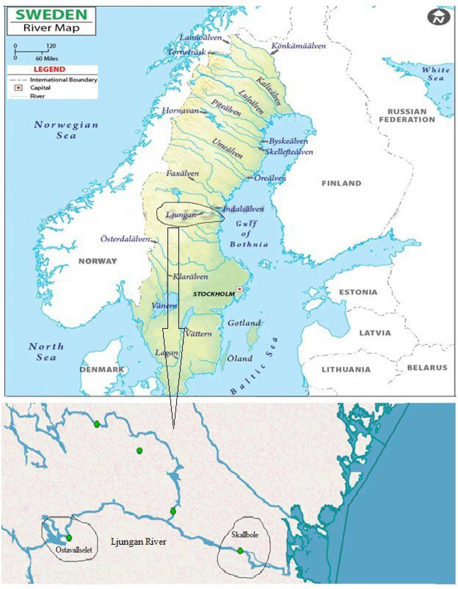
In this study, Ljungan River basin located in Sweden is chosen for case study (Figure 1). This basin originates from Trondheim and Norwegian border. The river is 399 km long and its catchment area drains Swedish counties of Jämtland and Västernorrland. The available flow estimation is crucial due to many hydropower power plants located along this basin. In addition, the river basin flows mostly through the coldest part of the country. Therefore, these points impute us to select this basin as a case study area in this study. For modeling and estimation of flows in this basin, two hydraulic stations data are selected as shown in Figure 1. To represent a better sketch of the available water estimation in the basin, one station is selected from upstream side of the basin, i.e., Ostavallselet station and another station is selected from the downstream side of the basin i.e., Skallbole station. Daily streamflow data of Ostavallselet station from 1 January 1976 to 8 June 2021 with a total value of 16,594 is obtained, whereas for Skallbole station, daily streamflow data from 1 January 1956 to 8 June 2021 with total values of 23,897 is collected. Data on unrecorded dates are excluded from the study. For application of models to streamflow data, data are divided into two partitions i.e., training and testing with a ratio of 80% and 20%, respectively. Brief data statistics of both hydrological stations are listed in Table 1. It can be seen that minimum and maximum values of data are included in the training dataset. Inclusion of lower and maximum values in the training dataset can be beneficial in the modeling procedure.
2.2. Artificial Neural Network (ANN)
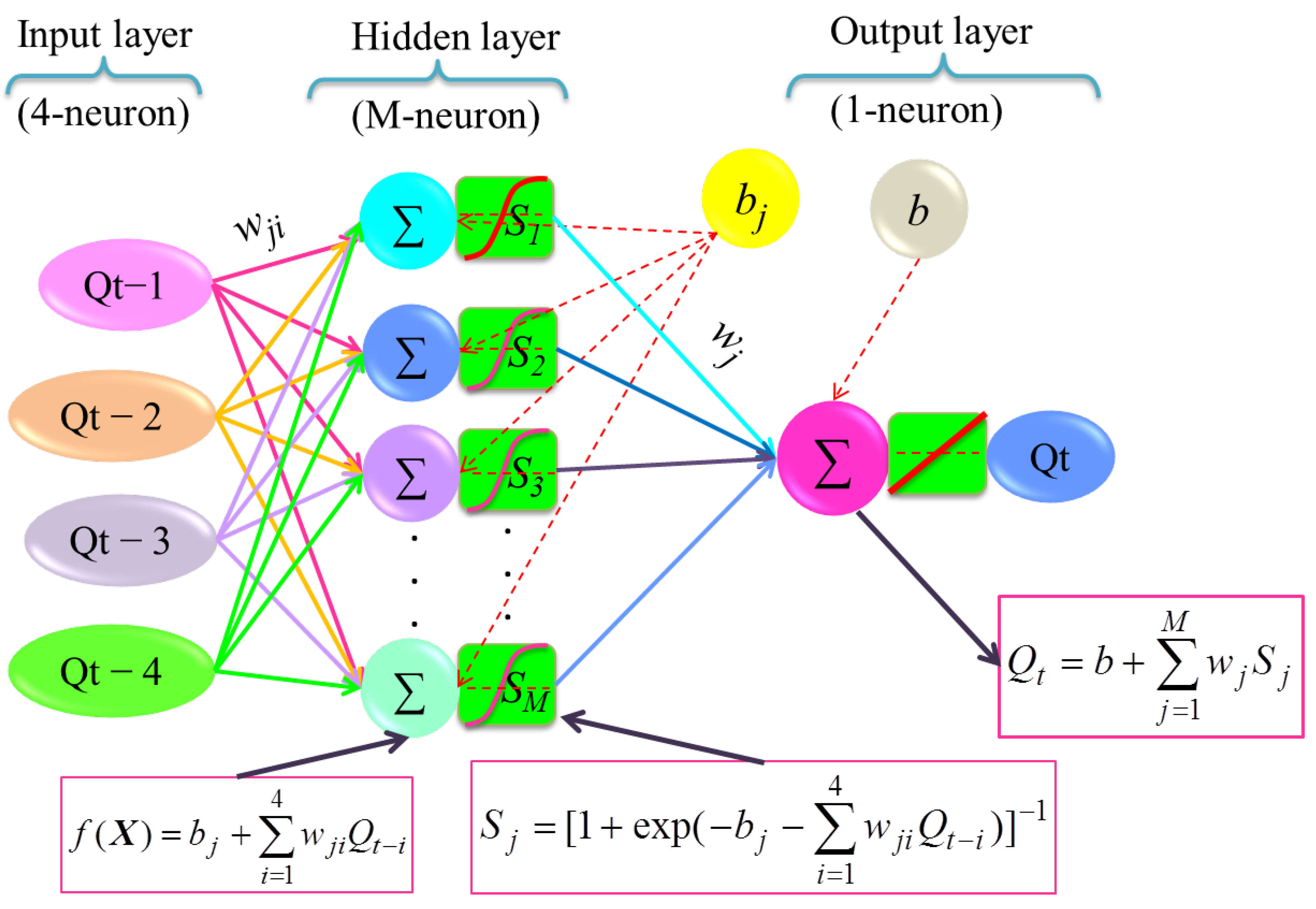
The output and input variables are connected with a nonlinear relation using artificial neural network (ANN) model. Generally, by providing a flexible nonlinear relation, the multilayer perceptron ANN (MLPNN) is a successful modelling approach [31,32]. Three layers are used for modelling scheme of MLPNN named input, hidden, and output layers as presented in Figure 2. The neurons (nodes) are the elements of every layer such as Qt−1, Qt−2, Qt−3, and Qt−4 and are used for input nodes as observed data and Qt is the node of output layer indicating forecasted variable (streamflow).
The databases in input and output nodes were normalized between −1 and 1 as below:
where QtN = normalized data of Qi i = t, t−1, t−2, t−3, t−4. The MLPNN provides a nonlinear map between inputs and output. The hidden nodes are directly used to join the nonlinear response of output nodes and the input nodes. The nonlinear relation of sigmoid function i.e., Sj is used to connect j- hidden node and input nodes of Qt−1, Qt−2, Qt−3, Qt−4 and bj is named bias and wji are the weights linking the j-th hidden node and i-th input node (i = 1,…,4 and j = 1,…,M). As presented in Figure 2, b and wj are respectively the bias, weights of j- hidden node which are applied to connect the output node and hidden nodes.
It is a challenge to provide the best connections of input and output nodes using biases (b) and weights (w). The learning method for computing the optimal connection parameters i.e., w and b are important for providing the accurate approximation. The back-propagation (BP) approach is a popular learning method used to train the ANN model. In this study for high-speed convergence [33], Levenberg–Marquardt (LM) training method is utilized for learning scheme of MLPNN. MATLAB toolbox of ANN machine learning is implemented for providing the ANN models trained by LM algorithm.
2.3. Radial Basis Function Neural Network (RBFNN)
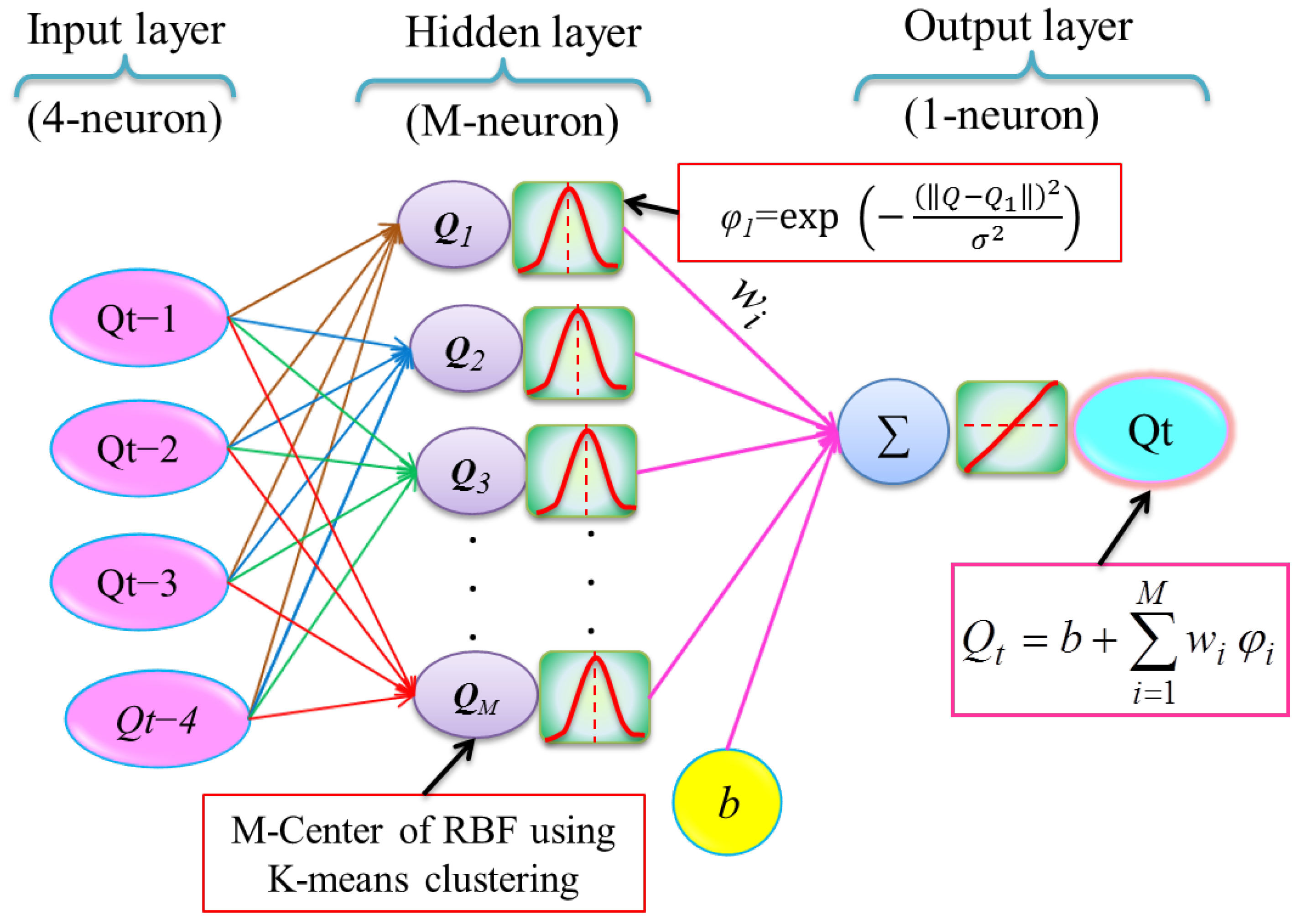
The ANN model using radial basis function (RBF) is a well-known ML approach with efficient training scheme [34]. The modelling structure of RBFNN applied in Figure 3 shows that this model involves three layers similar to the MLPNN but has no weight between input and hidden nodes and has Gaussian functions in the hidden nodes. The output node is connected with M-hidden nodes based on the weights and bias as unknown coefficients presented in Figure 3.
As seen from the Figure 3, is Gaussian function or RBF which is applied for nonlinear transformation of the input data, wi is the connected weight between i-th hidden node and output node. are the centers of RBF i.e.,
and is the shape parameter of RBF.
Center ( and are the main parameters for Gaussian function or RBF. By increasing the distance of a point () from i-center of RBF (), the values of the RBF decrease. Thus, the center of RBF is a controlling parameter of the model for providing a nonlinear relation that the M-center for RBF is determined using K-means clustering by using MATALB software in the modelling process. The shape parameter of the RBF is manually selected. It has M + 1 weights and bias as presented in Figure 3. Therefore, it should be trained for calibrating the unknown coefficients as the best connection between the input nodes and output node. Center ( and are determined by minimizing the mean square error between observed and predicted data in the training phase. Thus, modeling with RBFNN has three steps: (i) Giving the control parameters of the models (e.g., number of hidden nodes, shape factor ), (ii) determining the center for hidden nodes using K-means clustering method, (iii) training the RBFNN model for determining weights using last square approach.
2.4. Multivariate Adaptive Regression Spline (MARS)
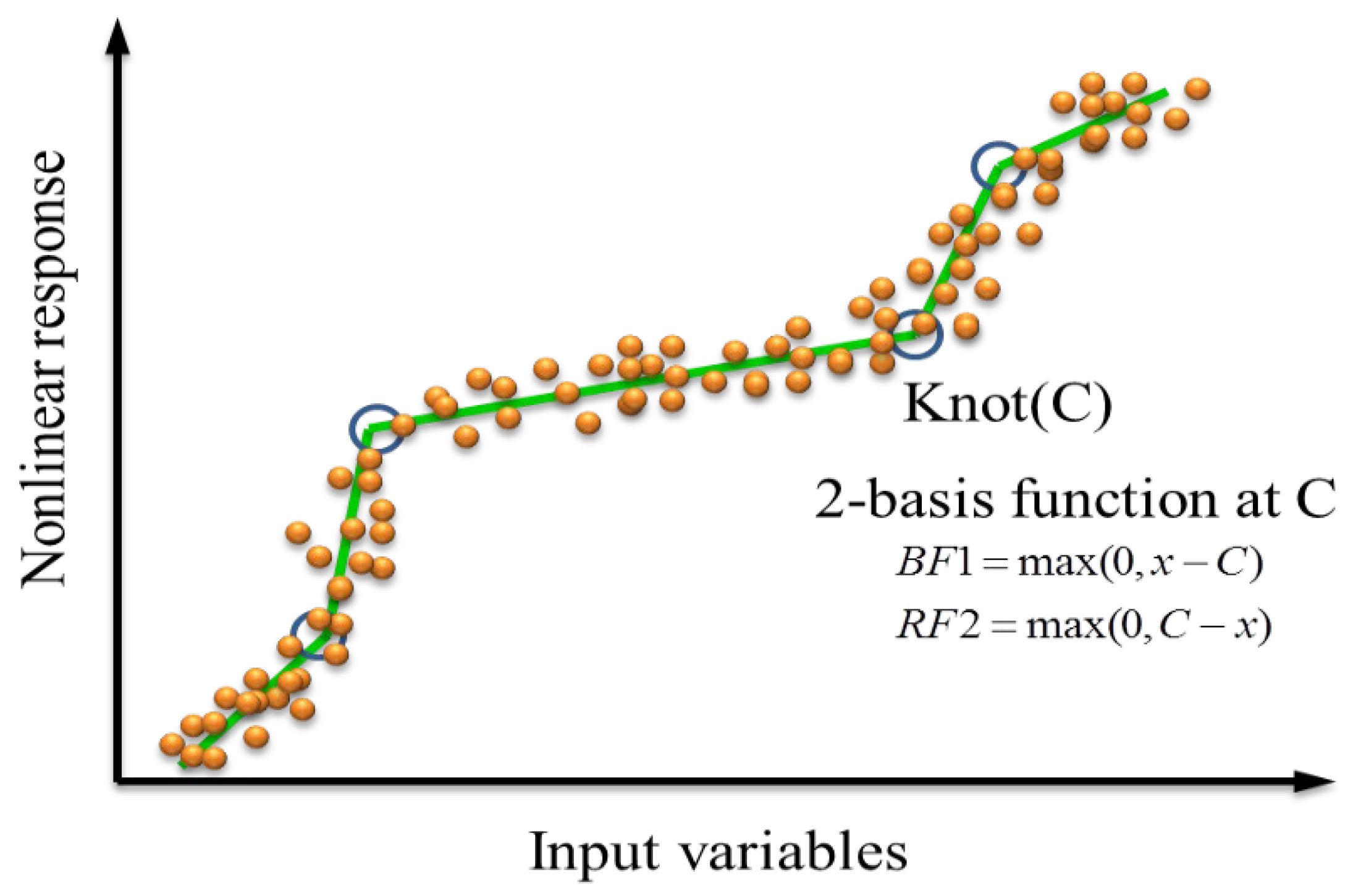
MARS is a well-known nonparametric prediction tool which provides a nonlinear relation using splines [35]. Recently, the MARS has acceptable applications to forecast streamflow of semi-arid region [36] and to predict the monthly streamflow of Swat River located at Pakistan [37]. Using piecewise linear splines basis function (BF), the MARS relation is determined as below:
where b and wi are unknown coefficients, bias, and weights, respectively. The weights are utilized to join m - BF. Piecewise linear function is given as below:
where Ci is a knot for i-th BF that it is defined as a piecewise linear function using knot of C which is presented in Figure 4. The positive part of BF is considered by max () term of two parts of BF on Equation (3). The MARS algorithm involves two phases named (i) forwarding step and (ii) backward phase. The forward phase is used to find the knots using randomly position in domain of the inputs where BF for each knot is computed in this part. Until maximum inputs are determined, selecting knot is repeated in the first phase. The backward phase is used to delete the BFs with insignificant effects [38,39]. The BF obtained in the first phase are explored using a stepwise process, thus we can represent the BF by a multiplying truncated function as follows:
in which K denotes number of knots, Ski indicates the right/left step function given 1/–1, is input i at knot k, and Cki denotes knot location. The generalized cross-validation as a simple selecting approach is utilized to determine the effective subset models as BF in MARS.
2.5. M5 Model Tree
A machine learning method as subset-data-driven is applied in M5 tree model (M5Tree). The tree structure is implemented as a framework of data-driven procedure in M5tree model that this tree framework is constructed using input and output databases [40,41]. In tree structure, linear equation is used. In M5Tree, we have root, nodes, branches, and leaves similar to structure of a real tree. Two phases are implemented to build a tree model including i) the decision tree for designing the nodes, branches, and leaves of tree using input database and ii) shrink the designed tree model for controlling the overfitted tree and by pruning the branches, replacing the branches and leaves with a linear functions [42].
The nodes are determined by split criterion using maximization of reduction of standard deviation (SDR) as below.
where Q denotes a set of samples included in a node, Qi is a subset with ith potential test samples, and Sd represents standard deviation for input data. A node will not be cut, when SDR of data at node is impossible, thus, it is provided as the end process to provide a node or leaf. Offspring nodes provide more accurate predictions than parent nodes due to less standard deviation with higher homogeneity on classification process of M5tree model. M5tree can be provided with a relation with minimum error and high-accuracy when almost possible nodes and branches are examined in selecting the model process.
2.6. Radial M5 Model Tree
To provide a smooth prediction and to control the active region of inputs, a modified version of M5Tree model named radial basis M5Tree (RM5Tree) was proposed for structural reliability analysis [43]. The RM5Tree showed the successful application for prediction of complex problems such as river suspended sediment [44] and reference evapotranspiration [45]. In RM5Tree, the input variables are transferred from real space into radial space using a kernel function [46] and the radial inputs are used for modelling of streamflow. RM5Tree model has three main layers named input layer, transfer layer, and M5tree model layer. In input layer, the inputs are normalized as follows [47]:
where, and are mean and STD of input Q, respectively. In the second layer named transferring layers, we used several radial number functions (NF), manually. The NF represents the inputs in radial space and the inputs of M5Tree are controlled by this factor. Therefore, it is a map of input data from X-space with n-dimension (e.g., 2–4 inputs in current paper) to radial-space with NF- dimension. The input data in training phase is transferred by radial basis function (RBF) as follows:
where, σ is the shape parameter of RBF as Kernel function. The NV-inputs are transferred from real-space into NF-space with Kernel function. Thus, the center and σ of Kernel function provided in this radial transformation are controlling parameters of the model. is provided a smooth property corresponding to NF-input that is considered as 0.5 for all models and C represents center of RBF which is randomly selected from feasible domain of inputs. is normalized input obtained by Equation (6). n and NF respectively denote the number of data for training and number of nodes for RBF, thus . By using Equation (7), we have a map for NF- center point as below:
where, n is number of data, NV is number of inputs in real space, and NF is number of inputs in radial space. Gaussian function is used for nonlinear map and number of center points controlled the smooth prediction of M5Tree models. The following steps are used in the second layer of RM5tree modes: (i) Random generation of NF- center point from domain of as C = [Zmin Zmax] and (ii) transformation of input data form NV variables from real-space into NF inputs using RBF for each center given in step i.
In the third layer, we applied the M5Tree model for calibrating the streamflow using the inputs provided by the second layer by nonlinear map of using Equation (7).
2.7. Comparative Matrix
The accuracies of studied models were assessed using the following statistics:
where Qc and Q0 are the computed and observed streamflow and is the mean observed streamflow and N is the quantity of data.
3. Application and Results
The RM5Tree, M5Tree, ANN, RBFNN, and MARS methods were compared in streamflow prediction using daily data from two stations, Ostavallselet (upstream) and Skallbole (downstream), Sweden. First, the optimal input lags were determined using MARS method and four previous streamflow values were used as input. Then, all five methods were compared using this input combination.
Table 2 presents the training and testing results of MARS method in prediction streamflow of Ostavallselet Station. In the table, Qt−1 shows the streamflow at t−1 (one previous day) and target value is Qt. It is apparent from Table 2 that the MARS model with 3rd input combination (Qt−1, Qt−2, Qt−3) has the lowest RMSE (11.87 in training and 13.27 in testing), MAE (7.11 in training and 8.43 in testing), MAPE (0.940 in training and 0.913 in testing), and the highest NSE (0.725 in training and 0.683 in testing).
Next, RM5Tree, M5Tree, ANN, RBFNN and MARS will be compared in predicting streamflow of Ostavallselet Station using 3rd input combination. The comparison outcomes are summed up in Table 3 in terms of RMSE, MAE, MAPE, and NSE. As seen from the table, the RM5tree has the best accuracy in predicting streamflow of Ostavallselet Station, while the M5Tree provides the worst outcomes in the testing stage. In the training stage, the RM5Tree model provides the lowest RMSE (9.36), MAE (5.25), MAPE (0.939), and highest NSE (0.798) which indicates that this method has better approximation (fitting) ability compared to other four methods.
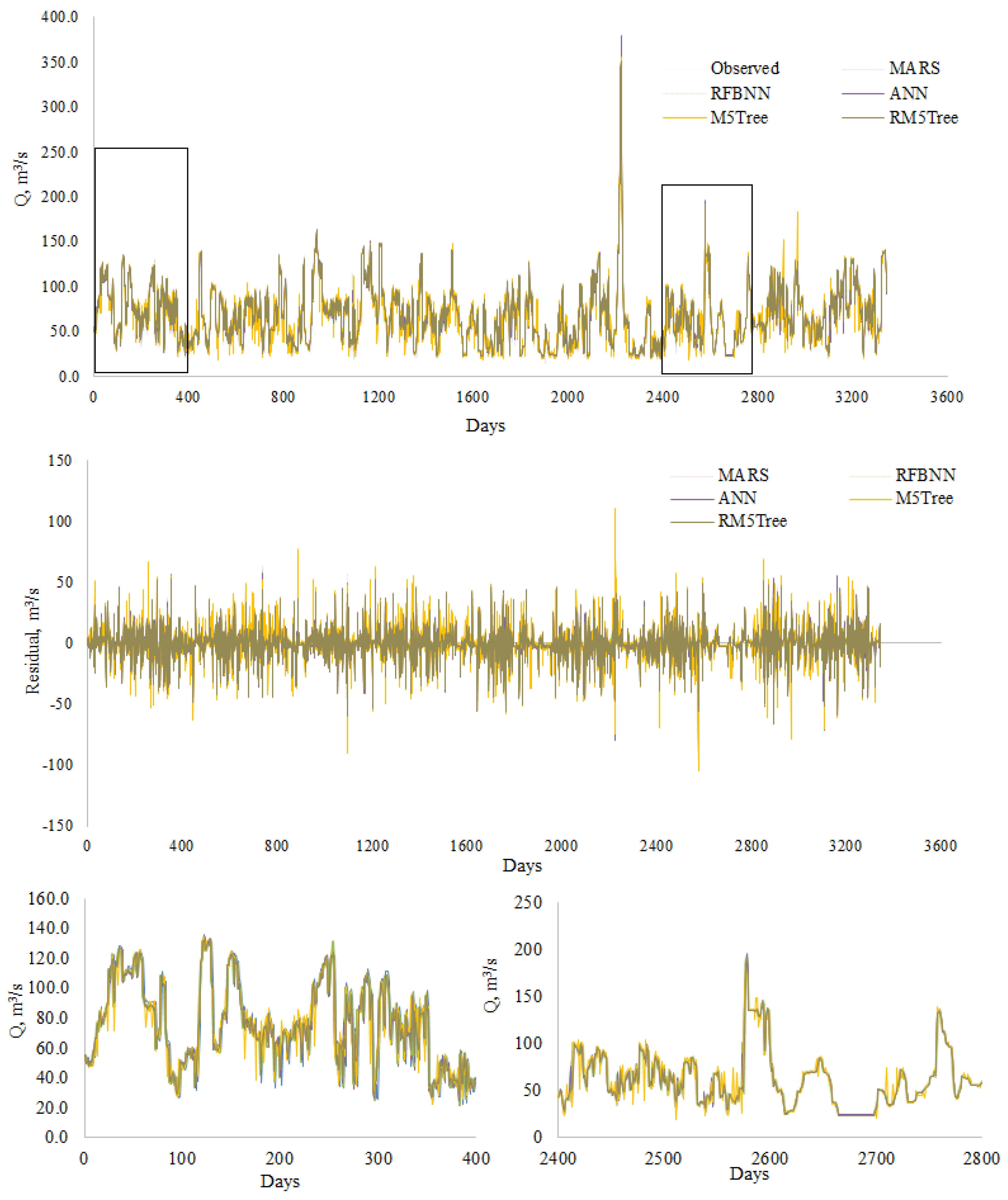
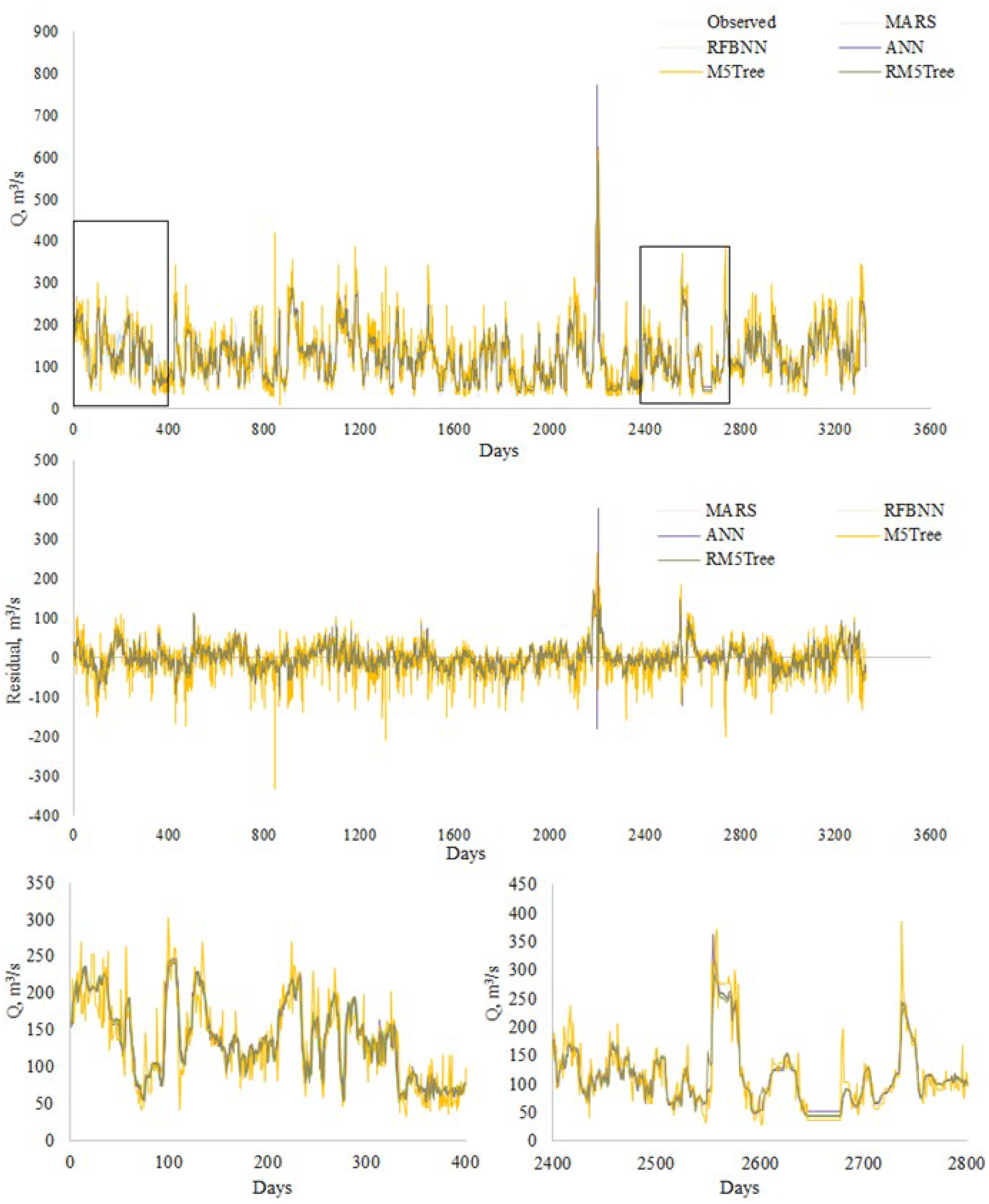
The fitting accuracy of the MARS, RBFNN, and ANN and M5Tree is similar while the testing accuracy of the M5Tree is worse than the other three models. The RM5Tree has the best accuracy in predicting streamflow of Ostavallselet Station in the testing stage with the lowest RMSE (12.54), MAE (8.19), MAPE (0.874) and highest NSE (0.692). The RM5Tree improves the accuracy of M5Tree by 18.8, 26.4, 1.5, and 10.1% with respect to RMSE, MAE, MAPE, and NSE in the training stage, while the corresponding improvements in the testing stage are 26.5, 17.9, 5.9, and 10.9%, respectively. Figure 5 illustrates the time variation graphs of the observed and predicted streamflow by RM5Tree, M5Tree, ANN, RBFNN, and MARS models for the test period of Ostavallselet Station. Two figures at the lower part focus on the two frames indicated in the main graph. Time variation of residuals are also provided in this figure to clearly see the differences among the applied models. As can be observed from the residual and detail graphs below, the predictions of the RM5Tree follow the observed values closer than the other four models.
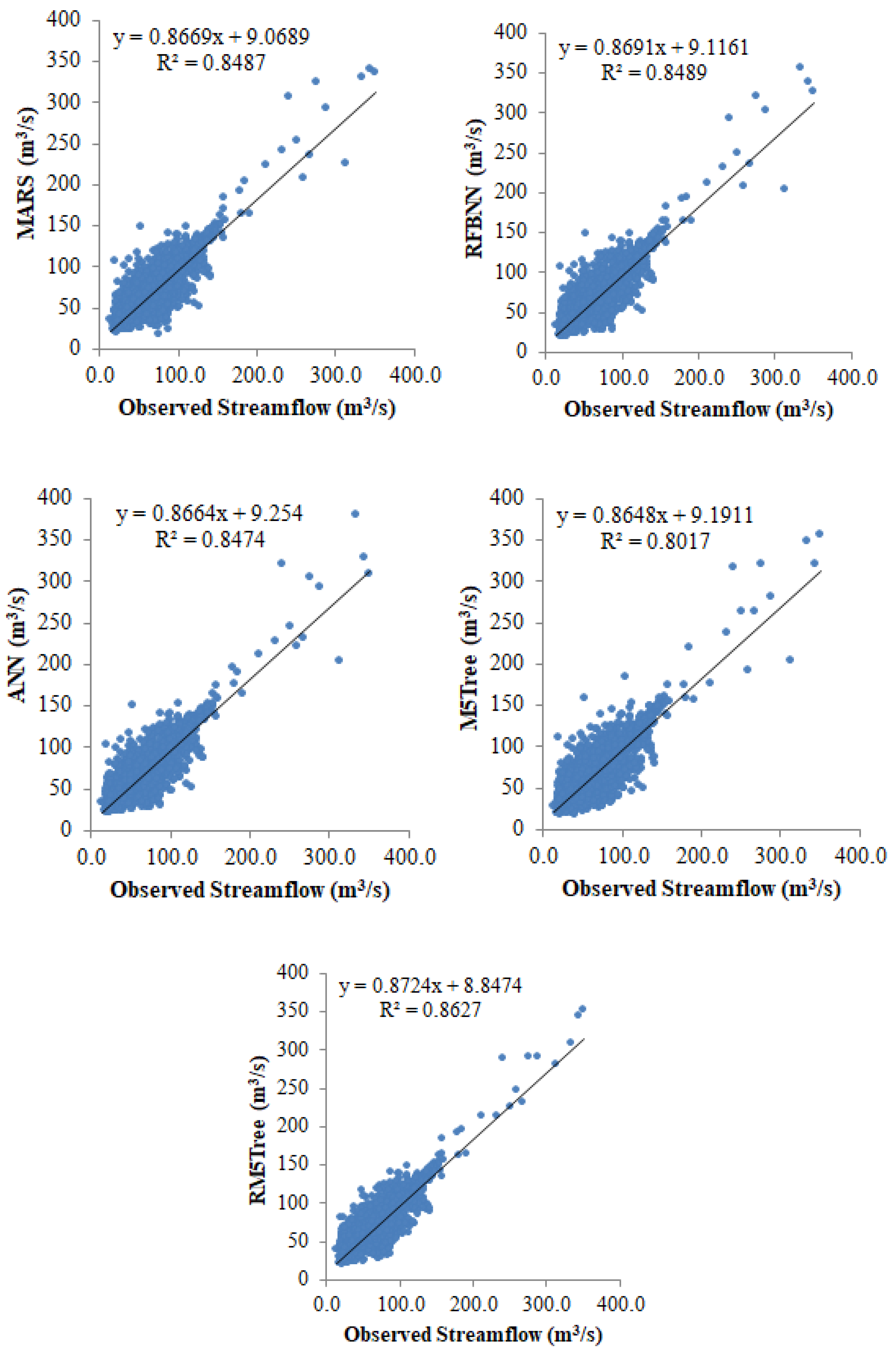
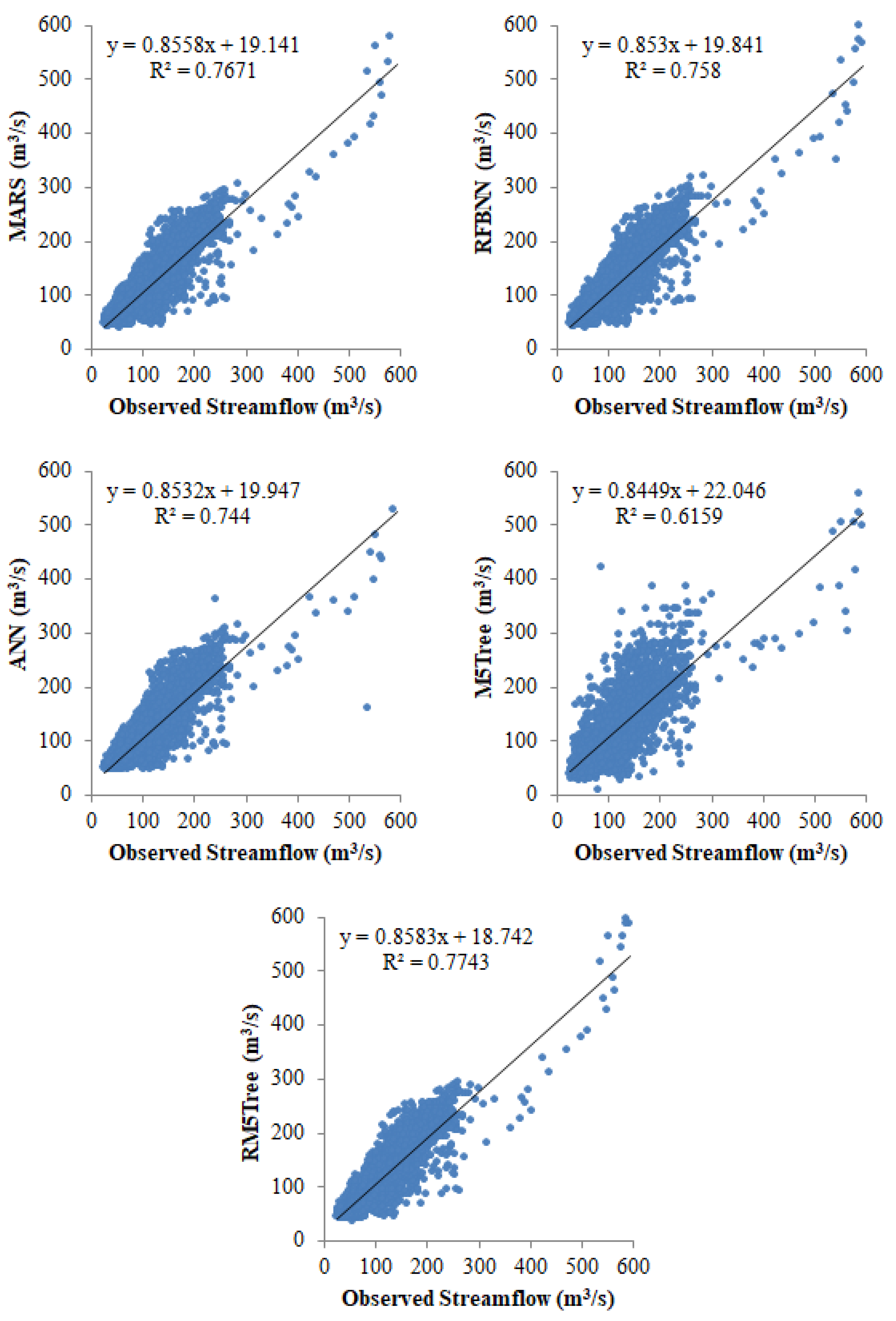
Scatterplots of the observed and predicted streamflow of Ostavallselet Station are given in Figure 6 for the test period. It is apparent from the figure that less scattered predictions belong to RM5Tree and slope and bias coefficients of the fit line for this model are closer to the 1 and 0 and it has higher R2 (0.8627) compared to the other four models.
Training and testing results of the MARS models for different input combinations composed of different streamflow lags of Skallbole Station are provided in Table 4. As seen from the table, the MARS model with inputs of Qt−1, Qt−2 (2nd input case) has the best accuracy (RMSE: 15.25, MAE: 10.89, MAPE: 0.097, NSE: 0.738). Table 5 compares the five implemented methods in predicting streamflow of Skallbole Station for the optimal input combination.
It is evident from the evaluation statistics, the RM5Tree model has the best accuracy in both training and testing stages with the lowest RMSE (11.25), MAE (6.87), MAPE (0.060) and the highest NSE (0.869) in training and the lowest RMSE (15.07), MAE (10.86), MAPE (0.097) and the highest NSE (0.745) in testing.
The accuracy of the M5Tree was improved by 13.1, 6.9, 4.8, and 1.6% with respect to RMSE, MAE, MAPE, and NSE applying RM5Tree model in the training stage whereas the corresponding percentages are 1.6, 0.8, 1, and 1.8% for the testing stage, respectively.
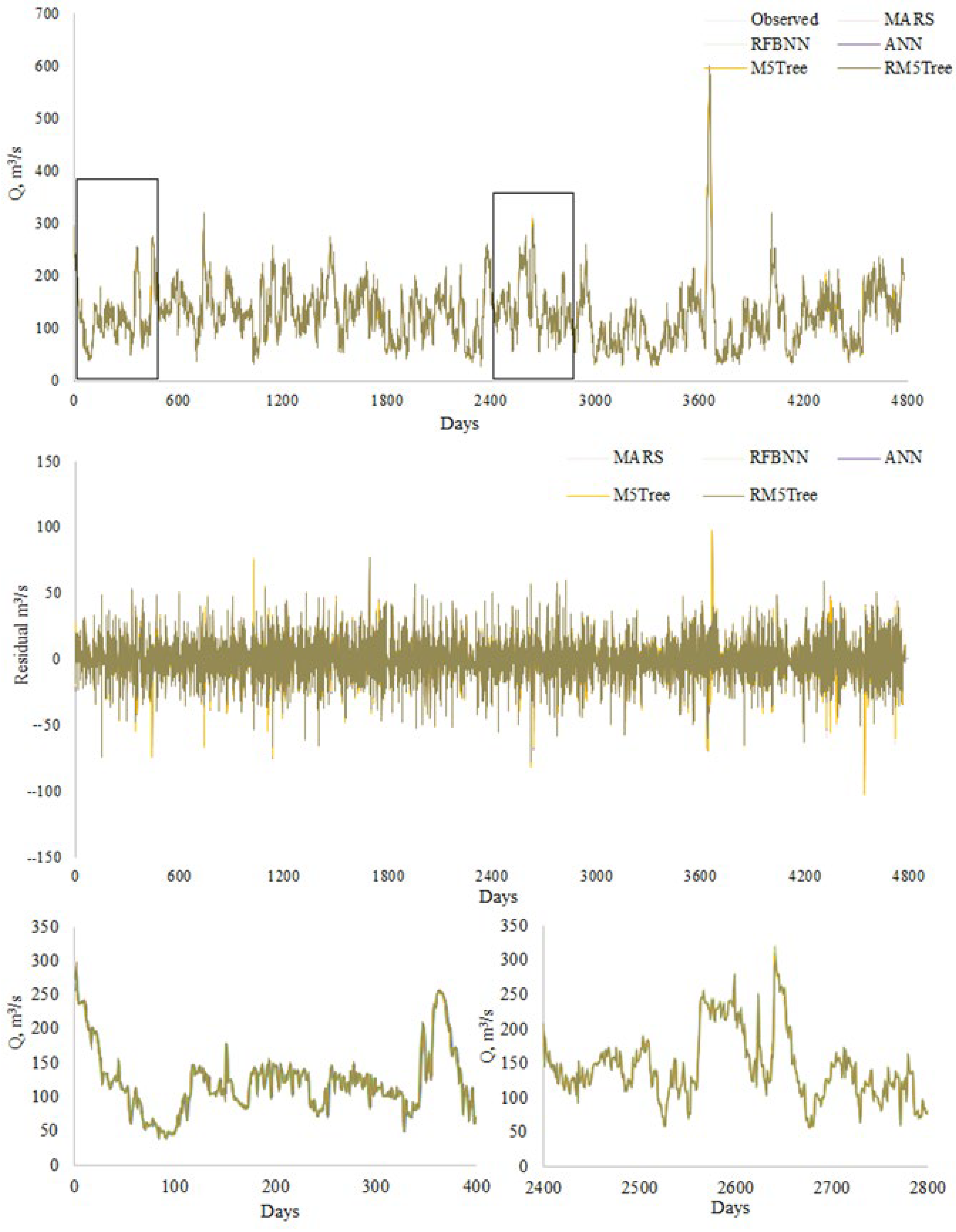
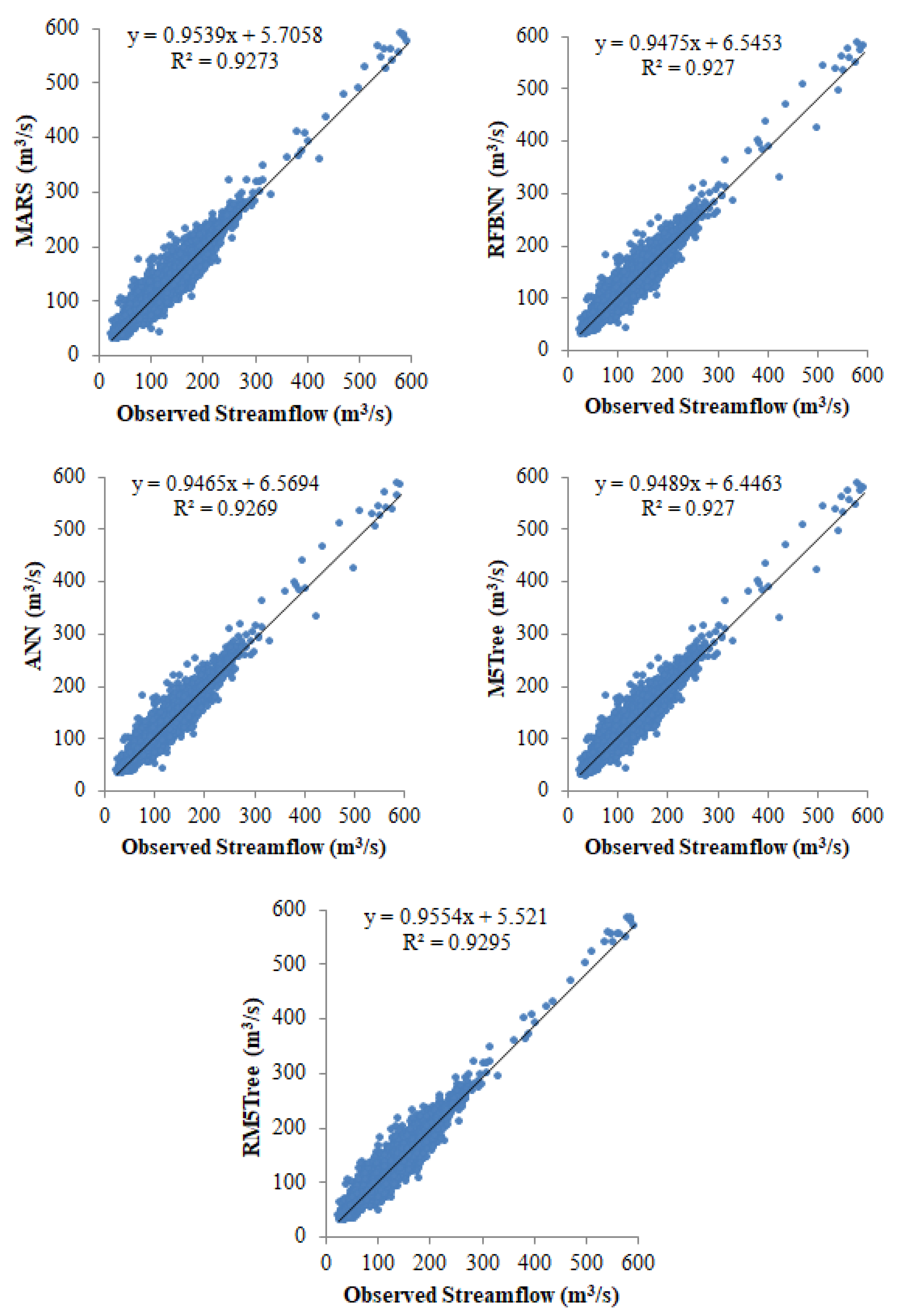
Observed and predicted streamflow values of Skallbole Station are visually compared in Figure 7 in the form of hydrograph. Here also closer predictions of RM5Tree are seen especially from the residual and detail graphs. It is clear from the scatterplots in Figure 8 that the RM5Tree model has the least scattered predictions followed by the MARS model.
The RM5Tree, M5Tree, ANN, RBFNN, and MARS methods were also compared in estimating the streamflow of Skallbole Station (downstream) using data of Ostavallselet Station (upstream). The MARS method was also employed here to select the optimal input combination. Training and testing statistics of the MARS models are summed up in Table 6.
Among the input combinations, the fourth one provides the lowest RMSE (30.15), MAE (22.07) and MAPE (0.202) and the highest NSE (0.506) in estimating streamflow of downstream station using data of upstream station. Thus, this combination was used to compare the RM5Tree, M5Tree, ANN, RBFNN, and MARS methods and corresponding statistics were provided in Table 7. As clearly observed from the table, the RM5Tree performed superior to the other models in estimating streamflow of downstream station using data of upstream station.
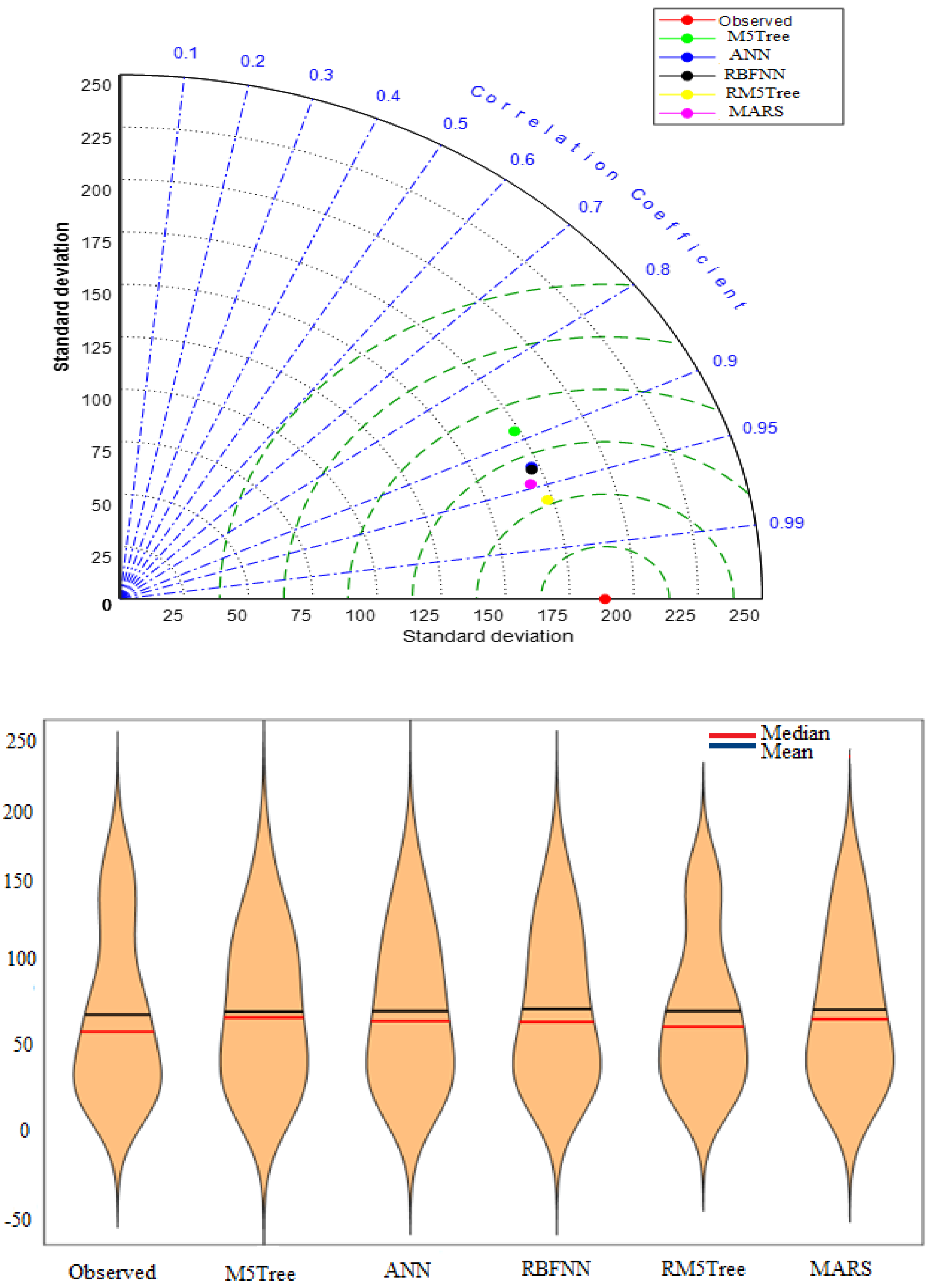
The relative improvements in RMSE, MAE, MAPE, and NSE of the M5Tree model are 30.6, 28.3, 28, and 55.8% applying RM5Tree model in the testing period, respectively. Figure 9 illustrates the time variation graphs of the observed and estimated streamflow of downstream station using upstream data. It is observed from the graphs that the RM5Tree estimates follow the observed streamflow values better than the M5Tree, ANN, RBFNN, and MARS models. It is also evident from Figure 10 that the RM5Tree produces less scattered estimates with higher determination coefficient than the other four methods and the M5Tree has the worst outcomes. Taylor and violin diagrams provided in Figure 11 also demonstrated that the RM5Tree model has closer standard deviation to the observed streamflow data and it has the lowest RMSE and the highest correlation.
4. Discussion
The aim of our study was to present a new modelling strategy based on the use of MARS for deciding the best input variables and a new model, RM5Tree, for forecasting daily streamflow. The results revealed that the MARS method can be successfully employed for input selection process. The assessment criteria and graphical inspection methods indicated that the RM5Tree method has superiority over other implemented methods (ANN, RBFNN, MARS, and M5Tree) in daily streamflow forecasting.
The main limitation of this study is the limited available data. This study only used streamflow data as input and data from two stations were used, therefore, the results could not be generalized. On the other hand, the effect of other climatic parameters and or basin parameters could not be investigated because of lack of such data. Predicting streamflow in cold climate regions presents a challenge since the natural processes in such basins are highly variable both seasonally and annually. This variability is mainly dependent on topo-geomorphological and climatic conditions of the basin. This causes uncertainty in the models implemented and a major limitation in streamflow prediction in cold climate regions which are often poorly gauged or ungauged [48].
The overall results revealed that the M5Tree model acted worse than the other models in prediction of streamflow. This can be explained by the linear structure of this model. This characteristic prevents the method to adequately simulate streamflow which has complex behavior in cold climate. The main advantage of the RM5Tree model is the fact that the input data in training phase are transferred by radial basis function and thus, the model can map the nonlinear behavior compared to M5Tree. From quantitative and graphical comparison, it was observed that the models are much more successful in predicting streamflow of upstream station (Ostavallselet). This can be explained by the higher basin area of downstream station and streamflow here might be more complex because of different basin parameters (e.g., tributaries, agricultural use, soil moisture condition, land use land cover, dams and snow melting).
5. Conclusions
By this study, the ability of RM5Tree was tested in predicting and estimating streamflow of a cold climate. The method was compared with ANN, RBFNN, MARS, and M5Tree using daily data of two stations, Skallbole Station (downstream) and Ostavallselet Station (upstream), form Sweden. The outcomes of the study present the following conclusions:
- -
- It was observed that the RM5Tree method is very successful and it performs better than the other four methods in predicting the streamflow in both stations.
- -
- The RM5Tree considerably improved the accuracy of M5Tree; improvements in RMSE, MAE, MAPE, and NSE in testing stage are 26.5, 17.9, 5.9 and 10.9% for the Ostavallselet and 1.6, 0.8, 1, and 1.8% for the Skallbole, respectively.
- -
- The RM5Tree method performed superior to the ANN, RBFNN, MARS, and M5Tree in estimating the streamflow of the downstream (Skallbole) station using data of the upstream station (Ostavallselet); the RMSE, MAE, MAPE, and NSE of the M5Tree model were improved by 30.6, 28.3, 28, and 55.8% in the testing period by applying RM5Tree model, respectively. Although RM5Tree provided better prediction results for streamflow forecasting, this study still has some limitations. The main limitation is the less data inputs usage for modeling streamflow variable. The streamflow variable not only depends on the previous values of streamflow, but also on other climatic variables. Therefore, in future studies, other climatic variables data can be also used to model the streamflow process.
Author Contributions
Conceptualization: R.M.A., O.K., and B.K. Formal analysis: B.K., S.H., and O.K. Validation: O.K., B.K., R.M.A., S.H., and J.P. Supervision: O.K. and B.K. Writing original draft: O.K., B.K., S.H., J.P., and R.M.A. Visualization: R.M.A. and B.K. Investigation: B.K., S.H., and J.P. All authors have read and agreed to the published version of the manuscript.
Funding
This research received no external funding.
Institutional Review Board Statement
Not applicable.
Informed Consent Statement
Not applicable.
Data Availability Statement
The data presented in this study will be available upon reasonable request from the corresponding author.
Conflicts of Interest
There is no conflict of interest in this study.
References
- McInerney, D.; Thyer, M.; Kavetski, D.; Laugesen, R.; Woldemeskel, F.; Tuteja, N.; Kuczera, G. Seamless streamflow model provides forecasts at all scales from daily to monthly and matches the performance of non-seamless monthly model. Hydrol. Earth Syst. Sci. Discuss. 2022, 1, 1–22. [Google Scholar] [CrossRef]
- Shen, Y.; Wang, S.; Zhang, B.; Zhu, J. Development of a stochastic hydrological modeling system for improving ensemble streamflow prediction. J. Hydrol. 2022, 608, 127683. [Google Scholar] [CrossRef]
- Chernos, M.; MacDonald, R.; Straker, J.; Green, K.; Craig, J. Simulating the cumulative effects of potential open-pit mining and climate change on streamflow and water quality in a mountainous watershed. Sci. Total Environ. 2021, 806, 150394. [Google Scholar] [CrossRef] [PubMed]
- Jia, B.; Zhou, J.; Tang, Z.; Xu, Z.; Chen, X.; Fang, W. Effective stochastic streamflow simulation method based on Gaussian mixture model. J. Hydrol. 2021, 605, 127366. [Google Scholar] [CrossRef]
- Liu, Y.; Ji, C.; Wang, Y.; Zhang, Y.; Hou, X.; Xie, Y. Quantifying streamflow predictive uncertainty for the optimization of short-term cascade hydropower stations operations. J. Hydrol. 2021, 605, 127376. [Google Scholar] [CrossRef]
- Hunt, K.M.; Matthews, G.R.; Pappenberger, F.; Prudhomme, C. Using a long short-term memory (LSTM) neural network to boost river streamflow forecasts over the western United States. Hydrol. Earth Syst. Sci. Discuss. 2022, volume 1, 1–30. [Google Scholar] [CrossRef]
- Towler, E.; Woodson, D.; Baker, S.; Ge, M.; Prairie, J.; Rajagopalan, B.; Shanahan, S.; Smith, R. Incorporating Mid-Term Temperature Predictions into Streamflow Forecasts and Operational Reservoir Projections in the Colorado River Basin. J. Water Resour. Plan. Manag. 2022, 148, 04022007. [Google Scholar] [CrossRef]
- Hapuarachchi, H.; Bari, M.; Kabir, A.; Hasan, M.; Woldemeskel, F.; Gamage, N.; Feikema, P. Development of a national 7-day ensemble streamflow forecasting service for Australia. Hydrol. Earth Syst. Sci. Discuss. 2022, volume 2, 1–35. [Google Scholar] [CrossRef]
- Zhou, Y.; Cui, Z.; Lin, K.; Sheng, S.; Chen, H.; Guo, S.; Xu, C.-Y. Short-term flood probability density forecasting using a conceptual hydrological model with machine learning techniques. J. Hydrol. 2021, 604, 127255. [Google Scholar] [CrossRef]
- Wegayehu, E.B.; Muluneh, F.B. Short-Term Daily Univariate Streamflow Forecasting Using Deep Learning Models. Adv. Meteorol. 2022, 2022, 1–21. [Google Scholar] [CrossRef]
- Cho, K.; Kim, Y. Improving streamflow prediction in the WRF-Hydro model with LSTM networks. J. Hydrol. 2021, 605, 127297. [Google Scholar] [CrossRef]
- Essam, Y.; Huang, Y.F.; Ng, J.L.; Birima, A.H.; Ahmed, A.N.; El-Shafie, A. Predicting streamflow in Peninsular Malaysia using support vector machine and deep learning algorithms. Sci. Rep. 2022, 12, 1–26. [Google Scholar] [CrossRef] [PubMed]
- Liu, Y.; Hou, G.; Huang, F.; Qin, H.; Wang, B.; Yi, L. Directed graph deep neural network for multi-step daily streamflow forecasting. J. Hydrol. 2022, 607, 127515. [Google Scholar] [CrossRef]
- Afan, H.A.; Yafouz, A.; Birima, A.H.; Ahmed, A.N.; Kisi, O.; Chaplot, B.; El-Shafie, A. Linear and stratified sampling-based deep learning models for improving the river streamflow forecasting to mitigate flooding disaster. Nat. Hazards 2022, volume 1, 1–19. [Google Scholar] [CrossRef]
- Mehr, A.D.; Ghadimi, S.; Marttila, H.; Haghighi, A.T. A new evolutionary time series model for streamflow forecasting in boreal lake-river systems. Arch. Meteorol. Geophys. Bioclimatol. Ser. B 2022, volume 1, 1–14. [Google Scholar] [CrossRef]
- Hassan, S.A.; Khan, M.S. Climatic variability impact on river flow modeling of Chitral and Gilgit stations, Pakistan. Model. Earth Syst. Environ. 2022, volume 1, 1–11. [Google Scholar] [CrossRef]
- Samantaray, S.; Das, S.S.; Sahoo, A.; Satapathy, D.P. Monthly runoff prediction at Baitarani river basin by support vector machine based on Salp swarm algorithm. Ain Shams Eng. J. 2022, 13, 101732. [Google Scholar] [CrossRef]
- Zhou, P.; Li, C.; Li, Z.; Cai, Y. Assessing uncertainty propagation in hybrid models for daily streamflow simulation based on arbitrary polynomial chaos expansion. Adv. Water Resour. 2021, 160, 104110. [Google Scholar] [CrossRef]
- Nguyen, D.H.; Le, X.H.; Anh, D.T.; Kim, S.-H.; Bae, D.-H. Hourly streamflow forecasting using a Bayesian additive regression tree model hybridized with a genetic algorithm. J. Hydrol. 2022, 606, 127445. [Google Scholar] [CrossRef]
- Khosravi, K.; Golkarian, A.; Tiefenbacher, J.P. Using Optimized Deep Learning to Predict Daily Streamflow: A Comparison to Common Machine Learning Algorithms. Water Resour. Manag. 2022, 36, 699–716. [Google Scholar] [CrossRef]
- Feng, Z.-K.; Shi, P.-F.; Yang, T.; Niu, W.-J.; Zhou, J.-Z.; Cheng, C.-T. Parallel cooperation search algorithm and artificial intelligence method for streamflow time series forecasting. J. Hydrol. 2022, 606, 127434. [Google Scholar] [CrossRef]
- Latifoğlu, L. The Performance Analysis of Robust Local Mean Mode Decomposition Method for Forecasting of Hydrological Time Series. Iran. J. Sci. Technol. Trans. Civ. Eng. 2022, volume 2, 1–20. [Google Scholar] [CrossRef]
- Ghaderpour, E.; Vujadinovic, T.; Hassan, Q.K. Application of the Least-Squares Wavelet software in hydrology: Athabasca River Basin. J. Hydrol. Reg. Stud. 2021, 36, 100847. [Google Scholar] [CrossRef]
- Zamrane, Z.; Mahé, G.; Laftouhi, N.-E. Wavelet Analysis of Rainfall and Runoff Multidecadal Time Series on Large River Basins in Western North Africa. Water 2021, 13, 3243. [Google Scholar] [CrossRef]
- Lian, Y.; Luo, J.; Wang, J.; Zuo, G.; Wei, N. Climate-driven Model Based on Long Short-Term Memory and Bayesian Optimization for Multi-day-ahead Daily Streamflow Forecasting. Water Resour. Manag. 2021, 36, 21–37. [Google Scholar] [CrossRef]
- Rahmani, F.; Fattahi, M.H. Association between forecasting models’ precision and nonlinear patterns of daily river flow time series. Model. Earth Syst. Environ. 2022, volume 1, 1–10. [Google Scholar] [CrossRef]
- Kisi, O.; Shiri, J.; Karimi, S.; Adnan, R.M. Three Different Adaptive Neuro Fuzzy Computing Techniques for Forecasting Long-Period Daily Streamflows. In Studies in Big Data; Springer Science and Business Media LLC: Singapore, 2018; pp. 303–321. [Google Scholar]
- Ahmed, A.A.; Deo, R.C.; Ghahramani, A.; Feng, Q.; Raj, N.; Yin, Z.; Yang, L. New Double Decomposition Deep Learning Methods for Stream-Flow Water Level Forecasting Using Remote Sensing Modis Satellite Variables, Climate Indices and Observations. 2022. Available online: https://papers.ssrn.com/sol3/papers.cfm?abstract_id=4002418 (accessed on 15 January 2022). [CrossRef]
- Kilinc, H.C.; Haznedar, B. A Hybrid Model for Streamflow Forecasting in the Basin of Euphrates. Water 2022, 14, 80. [Google Scholar] [CrossRef]
- Kilinc, H.C. Daily Streamflow Forecasting Based on the Hybrid Particle Swarm Optimization and Long Short-Term Memory Model in the Orontes Basin. Water 2022, 14, 490. [Google Scholar] [CrossRef]
- Yuan, X.; Chen, C.; Lei, X.; Yuan, Y.; Muhammad Adnan, R. Monthly runoff forecasting based on LSTM–ALO model. Stoch. Environ. Res. Risk Assess. 2018, 32, 2199–2212. [Google Scholar] [CrossRef]
- Adnan, R.M.; Mostafa, R.R.; Kisi, O.; Yaseen, Z.M.; Shahid, S.; Zounemat-Kermani, M. Improving streamflow prediction using a new hybrid ELM model combined with hybrid particle swarm optimization and grey wolf optimization. Knowledge-Based Syst. 2021, 230, 107379. [Google Scholar] [CrossRef]
- Rezaie-Balf, M.; Naganna, S.R.; Kisi, O.; El-Shafie, A. Enhancing streamflow forecasting using the augmenting ensemble procedure coupled machine learning models: Case study of Aswan High Dam. Hydrol. Sci. J. 2019, 64, 1629–1646. [Google Scholar] [CrossRef]
- Feng, B.-F.; Xu, Y.-S.; Zhang, T.; Zhang, X. Hydrological time series prediction by extreme learning machine and sparrow search algorithm. Water Supply 2021, 22, 3143–3157. [Google Scholar] [CrossRef]
- Wang, M.; Rezaie-Balf, M.; Naganna, S.R.; Yaseen, Z.M. Sourcing CHIRPS precipitation data for streamflow forecasting using intrinsic time-scale decomposition based machine learning models. Hydrol. Sci. J. 2021, 66, 1437–1456. [Google Scholar] [CrossRef]
- Adnan, R.M.; Liang, Z.; Heddam, S.; Zounemat-Kermani, M.; Kisi, O.; Li, B. Least square support vector machine and multivariate adaptive regression splines for streamflow prediction in mountainous basin using hydro-meteorological data as inputs. J. Hydrol. 2020, 586, 124371. [Google Scholar] [CrossRef]
- Kilinc, H.C.; Yurtsever, A. Short-Term Streamflow Forecasting Using Hybrid Deep Learning Model Based on Grey Wolf Algorithm for Hydrological Time Series. Sustain. 2022, 14, 3352. [Google Scholar] [CrossRef]
- Adnan, R.M.; Liang, Z.; Trajkovic, S.; Zounemat-Kermani, M.; Li, B.; Kisi, O. Daily streamflow prediction using optimally pruned extreme learning machine. J. Hydrol. 2019, 577, 123981. [Google Scholar] [CrossRef]
- Adnan, R.M.; Kisi, O.; Mostafa, R.R.; Ahmed, A.N.; El-Shafie, A. The potential of a novel support vector machine trained with modified mayfly optimization algorithm for streamflow prediction. Hydrol. Sci. J. 2022, 67, 161–174. [Google Scholar] [CrossRef]
- Adnan, R.M.; Mostafa, R.R.; Elbeltagi, A.; Yaseen, Z.M.; Shahid, S.; Kisi, O. Development of new machine learning model for streamflow prediction: Case studies in Pakistan. Stoch. Hydrol. Hydraul. 2021, 36, 999–1033. [Google Scholar] [CrossRef]
- Kişi, Özgür Streamflow Forecasting Using Different Artificial Neural Network Algorithms. J. Hydrol. Eng. 2007, 12, 532–539. [CrossRef]
- Adnan, R.M.; Yuan, X.; Kisi, O.; Yuan, Y. Streamflow forecasting using artificial neural network and support vector machine models. Am. Acad. Sci. Res. J. Eng. Technol. Sci. 2017, 29, 286–294. [Google Scholar]
- Piotrowski, A.P.; Napiorkowski, J. Optimizing neural networks for river flow forecasting—Evolutionary Computation methods versus the Levenberg–Marquardt approach. J. Hydrol. 2011, 407, 12–27. [Google Scholar] [CrossRef]
- Yaseen, Z.M.; El-Shafie, A.; Afan, H.A.; Hameed, M.; Mohtar, W.H.M.W.; Hussain, A. RBFNN versus FFNN for daily river flow forecasting at Johor River, Malaysia. Neural Comput. Appl. 2015, 27, 1533–1542. [Google Scholar] [CrossRef]
- Friedman, J.H. Multivariate adaptive regression splines. Ann. Stat. 1991, volume 2, 1–67. [Google Scholar] [CrossRef]
- Al-Sudani, Z.A.; Salih, S.; Sharafati, A.; Yaseen, Z.M. Development of multivariate adaptive regression spline integrated with differential evolution model for streamflow simulation. J. Hydrol. 2019, 573, 1–12. [Google Scholar] [CrossRef]
- Adnan, R.M.; Liang, Z.; Parmar, K.S.; Soni, K.; Kisi, O. Modeling monthly streamflow in mountainous basin by MARS, GMDH-NN and DENFIS using hydroclimatic data. Neural Comput. Appl. 2021, 33, 2853–2871. [Google Scholar] [CrossRef]
- Adnan, R.M.; Yuan, X.; Kisi, O.; Adnan, M.; Mehmood, A. Stream Flow Forecasting of Poorly Gauged Mountainous Watershed by Least Square Support Vector Machine, Fuzzy Genetic Algorithm and M5 Model Tree Using Climatic Data from Nearby Station. Water Resour. Manag. 2018, 32, 4469–4486. [Google Scholar] [CrossRef]
Figure 1.
Location map of selected stations.

Figure 2.
Structure of MLPNN for forecasting Qt.

Figure 3.
Structure of RBFNN model.

Figure 4.
Structure for MARS model.

Figure 5.
Time variation graphs of the observed and predicted streamflow by RM5Tree, M5Tree, RBFNN, ANN, and MARS models in the test period of Ostavallselet Station (upstream).
Figure 5.
Time variation graphs of the observed and predicted streamflow by RM5Tree, M5Tree, RBFNN, ANN, and MARS models in the test period of Ostavallselet Station (upstream).

Figure 6.
Scatterplots of the observed and predicted streamflow by RM5Tree, M5Tree, RBFNN, ANN, and MARS models in the test period of Ostavallselet Station (upstream).
Figure 6.
Scatterplots of the observed and predicted streamflow by RM5Tree, M5Tree, RBFNN, ANN, and MARS models in the test period of Ostavallselet Station (upstream).

Figure 7.
Time variation graphs of the predicted streamflow by RM5Tree, M5Tree, RBFNN, ANN, and MARS models in the test period of Skallbole Station (downstream).
Figure 7.
Time variation graphs of the predicted streamflow by RM5Tree, M5Tree, RBFNN, ANN, and MARS models in the test period of Skallbole Station (downstream).

Figure 8.
Scatterplots of the observed and predicted streamflow by RM5Tree, M5Tree, RBFNN, ANN, and MARS models in the test period of Skallbole Station (downstream).
Figure 8.
Scatterplots of the observed and predicted streamflow by RM5Tree, M5Tree, RBFNN, ANN, and MARS models in the test period of Skallbole Station (downstream).

Figure 9.
Time variation graphs of the observed and estimated streamflow of Skallbole Station (downstream) by RM5Tree, M5Tree, RBFNN, ANN, and MARS models in the test period using data of Ostavallselet Station (upstream).
Figure 9.
Time variation graphs of the observed and estimated streamflow of Skallbole Station (downstream) by RM5Tree, M5Tree, RBFNN, ANN, and MARS models in the test period using data of Ostavallselet Station (upstream).

Figure 10.
Time scatterplots of the observed and estimated streamflow of Skallbole Station (downstream) by RM5Tree, M5Tree, RBFNN, ANN, and MARS models in the test period using data of Ostavallselet Station (upstream).
Figure 10.
Time scatterplots of the observed and estimated streamflow of Skallbole Station (downstream) by RM5Tree, M5Tree, RBFNN, ANN, and MARS models in the test period using data of Ostavallselet Station (upstream).

Figure 11.
Taylor and violin diagrams by different models in the test period—Station 2 estimation using upstream data.
Figure 11.
Taylor and violin diagrams by different models in the test period—Station 2 estimation using upstream data.


Table 1.
The statistical parameters of the streamflow data.
| Ostavallselet Station (Upstream) | Skallbole Station (Downstream) | |||||
|---|---|---|---|---|---|---|
| Whole data | Training | Testing | Whole data | Training | Testing | |
| Min (m3/s) | 16 | 16 | 26.4 | 7.20 | 7.20 | 14.4 |
| Max (m3/s) | 1050 | 1050 | 593 | 430 | 430 | 350 |
| Mean (m3/s) | 126.4 | 125.2 | 127.2 | 68.5 | 70.3 | 67.7 |
| Skewness | 65.7 | 77.9 | 56.4 | 36.4 | 38.1 | 34.2 |
| Std. dev. | 2.83 | 3.11 | 1.69 | 2.38 | 2.71 | 1.34 |
Table 2.
Training and testing statistics of the MARS models using different input combinations for daily streamflow prediction—Ostavallselet (upstream).
Table 2.
Training and testing statistics of the MARS models using different input combinations for daily streamflow prediction—Ostavallselet (upstream).
| Input Combinations | Training | Testing | ||||||
|---|---|---|---|---|---|---|---|---|
| RMSE (m3/s) | MAE (m3/s) | MAPE | NSE | RMSE (m3/s) | MAE (m3/s) | MAPE | NSE | |
| Qt−1 | 12.60 | 7.55 | 0.944 | 0.709 | 13.31 | 8.67 | 0.921 | 0.674 |
| Qt−1,Qt−2 | 12.19 | 7.42 | 0.947 | 0.714 | 13.45 | 8.70 | 0.919 | 0.673 |
| Qt−1,Qt−2, Qt−3 | 11.87 | 7.11 | 0.940 | 0.725 | 13.27 | 8.43 | 0.913 | 0.683 |
| Qt−1,Qt−2, Qt−3, Qt−4 | 12.16 | 7.33 | 0.948 | 0.717 | 13.29 | 8.48 | 0.921 | 0.681 |
Table 3.
Training and testing statistics of the RM5Tree, M5Tree, RBFNN, ANN, and MARS models in daily streamflow prediction using the optimal inputs of Qt−1, Qt−2, and Qt−3—Ostavallselet (upstream).
Table 3.
Training and testing statistics of the RM5Tree, M5Tree, RBFNN, ANN, and MARS models in daily streamflow prediction using the optimal inputs of Qt−1, Qt−2, and Qt−3—Ostavallselet (upstream).
| Methods | Training | Testing | ||||||
|---|---|---|---|---|---|---|---|---|
| RMSE (m3/s) | MAE (m3/s) | MAPE | NSE | RMSE (m3/s) | MAE (m3/s) | MAPE | NSE | |
| MARS | 11.87 | 7.11 | 0.940 | 0.725 | 13.27 | 8.43 | 0.913 | 0.683 |
| RBFNN | 11.82 | 7.10 | 0.951 | 0.726 | 13.26 | 8.41 | 0.921 | 0.685 |
| ANN | 11.68 | 7.05 | 0.952 | 0.728 | 13.32 | 8.44 | 0.921 | 0.682 |
| M5Tree | 11.53 | 7.13 | 0.953 | 0.725 | 17.07 | 9.98 | 0.929 | 0.624 |
| RM5Tree | 9.36 | 5.25 | 0.939 | 0.798 | 12.54 | 8.19 | 0.874 | 0.692 |
Table 4.
Training and testing statistics of the MARS models using different input combinations for daily streamflow prediction—Skallbole Station (downstream).
Table 4.
Training and testing statistics of the MARS models using different input combinations for daily streamflow prediction—Skallbole Station (downstream).
| Input Combinations | Training | Testing | ||||||
|---|---|---|---|---|---|---|---|---|
| RMSE (m3/s) | MAE (m3/s) | MAPE | NSE | RMSE (m3/s) | MAE (m3/s) | MAPE | NSE | |
| Qt−1 | 12.96 | 7.38 | 0.063 | 0.855 | 15.32 | 10.96 | 0.098 | 0.735 |
| Qt−1,Qt−2 | 11.40 | 6.91 | 0.062 | 0.864 | 15.25 | 10.89 | 0.097 | 0.738 |
| Qt−1,Qt−2, Qt−3 | 11.63 | 7.01 | 0.063 | 0.862 | 15.58 | 11.19 | 0.101 | 0.730 |
| Qt−1,Qt−2, Qt−3, Qt−4 | 11.37 | 6.92 | 0.062 | 0.864 | 15.42 | 11.04 | 0.099 | 0.734 |
Table 5.
Training and testing statistics of the RM5Tree, M5Tree, RBFNN, ANN, and MARS models in daily streamflow prediction using the optimal inputs of Qt−1 and Qt−2—Skallbole Station (downstream).
Table 5.
Training and testing statistics of the RM5Tree, M5Tree, RBFNN, ANN, and MARS models in daily streamflow prediction using the optimal inputs of Qt−1 and Qt−2—Skallbole Station (downstream).
| Methods | Training | Testing | ||||||
|---|---|---|---|---|---|---|---|---|
| RMSE (m3/s) | MAE (m3/s) | MAPE | NSE | RMSE (m3/s) | MAE (m3/s) | MAPE | NSE | |
| MARS | 11.40 | 6.91 | 0.062 | 0.864 | 15.25 | 10.89 | 0.097 | 0.738 |
| RBFNN | 12.95 | 7.41 | 0.064 | 0.854 | 15.30 | 10.93 | 0.098 | 0.728 |
| ANN | 12.89 | 7.41 | 0.064 | 0.854 | 15.31 | 10.90 | 0.098 | 0.731 |
| M5Tree | 12.95 | 7.38 | 0.063 | 0.855 | 15.31 | 10.95 | 0.098 | 0.732 |
| RM5Tree | 11.25 | 6.87 | 0.060 | 0.869 | 15.07 | 10.86 | 0.097 | 0.745 |
Table 6.
Training and testing statistics of the MARS models using different input combinations in estimating daily streamflow of Skallbole Station (downstream) using data from Ostavallselet Station (upstream).
Table 6.
Training and testing statistics of the MARS models using different input combinations in estimating daily streamflow of Skallbole Station (downstream) using data from Ostavallselet Station (upstream).
| Input Combinations | Training | Testing | ||||||
|---|---|---|---|---|---|---|---|---|
| RMSE (m3/s) | MAE (m3/s) | MAPE | NSE | RMSE (m3/s) | MAE (m3/s) | MAPE | NSE | |
| Qt−1 | 34.88 | 23.60 | 0.210 | 0.526 | 32.39 | 23.74 | 0.221 | 0.468 |
| Qt−1,Qt−2 | 33.71 | 22.57 | 0.200 | 0.546 | 30.74 | 22.42 | 0.203 | 0.498 |
| Qt−1,Qt−2, Qt−3 | 32.09 | 21.75 | 0.192 | 0.563 | 30.55 | 22.34 | 0.203 | 0.500 |
| Qt−1,Qt−2, Qt−3, Qt−4 | 33.25 | 22.09 | 0.193 | 0.556 | 30.15 | 22.07 | 0.202 | 0.506 |
Table 7.
Training and testing statistics of the RM5Tree, M5Tree, RBFNN, ANN, and MARS models in estimating daily streamflow prediction of Skallbole Station (downstream) using the optimal inputs of Qt−1, Qt−2, Qt−3, and Qt−4 from Ostavallselet Station (upstream).
Table 7.
Training and testing statistics of the RM5Tree, M5Tree, RBFNN, ANN, and MARS models in estimating daily streamflow prediction of Skallbole Station (downstream) using the optimal inputs of Qt−1, Qt−2, Qt−3, and Qt−4 from Ostavallselet Station (upstream).
| Methods | Training | Testing | ||||||
|---|---|---|---|---|---|---|---|---|
| RMSE (m3/s) | MAE (m3/s) | MAPE | NSE | RMSE (m3/s) | MAE (m3/s) | MAPE | NSE | |
| MARS | 33.25 | 22.09 | 0.193 | 0.556 | 30.15 | 22.07 | 0.202 | 0.506 |
| RBFNN | 32.93 | 21.91 | 0.192 | 0.560 | 30.18 | 22.03 | 0.199 | 0.507 |
| ANN | 32.30 | 21.69 | 0.191 | 0.564 | 31.41 | 22.38 | 0.202 | 0.499 |
| M5Tree | 33.23 | 22.03 | 0.191 | 0.557 | 41.84 | 29.61 | 0.268 | 0.337 |
| RM5Tree | 22.12 | 13.17 | 0.115 | 0.735 | 29.03 | 21.23 | 0.193 | 0.525 |
Publisher’s Note: MDPI stays neutral with regard to jurisdictional claims in published maps and institutional affiliations. |
© 2022 by the authors. Licensee MDPI, Basel, Switzerland. This article is an open access article distributed under the terms and conditions of the Creative Commons Attribution (CC BY) license (https://creativecommons.org/licenses/by/4.0/).
Share and Cite
MDPI and ACS Style
Kisi, O.; Heddam, S.; Keshtegar, B.; Piri, J.; Adnan, R.M. Predicting Daily Streamflow in a Cold Climate Using a Novel Data Mining Technique: Radial M5 Model Tree. Water 2022, 14, 1449. https://doi.org/10.3390/w14091449
AMA Style
Kisi O, Heddam S, Keshtegar B, Piri J, Adnan RM. Predicting Daily Streamflow in a Cold Climate Using a Novel Data Mining Technique: Radial M5 Model Tree. Water. 2022; 14(9):1449. https://doi.org/10.3390/w14091449
Chicago/Turabian StyleKisi, Ozgur, Salim Heddam, Behrooz Keshtegar, Jamshid Piri, and Rana Muhammad Adnan. 2022. "Predicting Daily Streamflow in a Cold Climate Using a Novel Data Mining Technique: Radial M5 Model Tree" Water 14, no. 9: 1449. https://doi.org/10.3390/w14091449
Note that from the first issue of 2016, this journal uses article numbers instead of page numbers. See further details here.