Mid-Channel Braid-Bar-Induced Turbulent Bursts: Analysis Using Octant Events Approach

Abstract

In a laboratory, a model of a mid-channel bar is built to study the turbulent flow structures in its vicinity. The present study on the turbulent flow structure around a mid-channel bar is based on unravelling the fluvial fluxes triggered by the bar’s 3D turbulent burst phenomenon. To this end, the three-dimensional velocity components are measured with the help of acoustic doppler velocimetry (ADV). The results indicate that the transverse component of turbulent kinetic energy cannot be neglected when analyzing turbulent burst processes, since the dominant flow is three-dimensional around the mid-channel bar. Due to the three-dimensionality of flow, the octant events approach is used for analyzing the flow in the vicinity of the mid-channel bar. The aim is to develop functional relationships between the stable movements that are modelled in the present study. To find the best Markov chain order to present experimental datasets, the zero-, first-, and second-order Markov chains are analyzed using the Akaike information criterion (AIC) and the Bayesian information criterion (BIC). The parameter transition ratio has evolved in this research to reflect the linkage of streambed elevation changes with stable transitional movements. For a better understanding of the temporal behaviors of stable transitional movements, the residence time vs. frequency graphs are also plotted for scouring as well as for depositional regions. The study outcome herein underlines the usefulness of the octant events approach for characterizing turbulent bursts around mid-channel bar formation, which is a precursor to the initiation of braiding configuration.

1. Introduction

The river Brahmaputra is well-known on the Indian subcontinent for its extreme braided condition. Braiding channel configuration is manifested in alluvial rivers in a high-fluvial-energy environment. Many academics have worked on describing the channel geometry of braided rivers and their channel plan shapes in the past. Nonetheless, in comparison to the wealth of literature on meandering systems, the underpinning causative factors of braiding initiation in alluvial streams have received relatively little attention.

The causative process of braiding in alluvial rivers is initiated by the formation of a mid-channel bar, which causes the bifurcation of streamflow into two courses in the inchoate stage of braided river development. The creation of mid-channel bars should be viewed as a precursor to the start of complicated braiding design. Several scholars have attempted to classify braided bar arrangement, employing criteria such as elongation, symmetry, and the appearance or exclusion of an avalanche face [1]. However, there is little consensus on these groupings, making clear categorization nearly impossible [1,2,3]. Due to the mutual interlinkages between sediment transport and water flow, morphological changes in braided streams are directly tied to bank erosion and deformation. The channel formation process in a braided stream begins with the emergence of bars under particular flow conditions due to the expansion of originally straight channels [4,5].

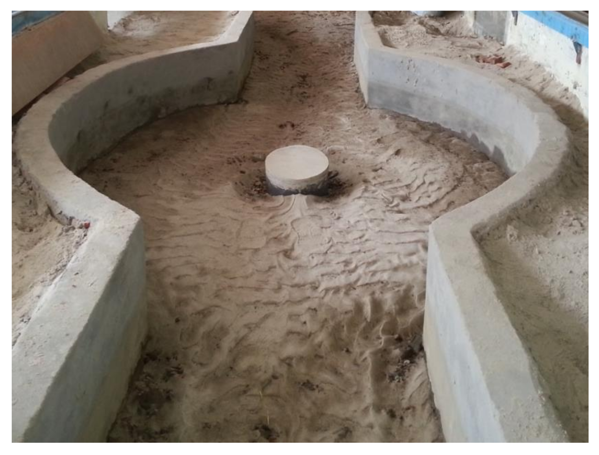
Several researches, namely [4,6,7,8], found that the creation and deformation of mid-channel bars in an alluvial channel are observed to be transient. Significantly, as observed by [1,2,3,4,6], the braiding behavior in alluvial streams originates from the initiation of the mid-channel bar, and that is the reason for selecting its study in the present research [9]. In a natural channel, the shape of the bar is non-uniform. For the sake of simplifying the experimental setup, the elliptical-shaped bar is configured in the model tray (Figure 1). The prime aim of the present study is to analyze the induced fluxes that are manifested in the turbulent structure due to the presence of a bar. Such analysis is focused on unraveling the inherent fluvial mechanics, which are primarily related to deposition and scouring in the proximity of the bar.

The authors of [10,11] had performed experiments in a turbulent open channel flow. They studied the space–time correlation structure of the bursting events using the conditional sampling technique. They observed that the temporal and spatial scale of sweep events extend more toward downstream than upstream.

The studies by [12,13] observed that a turbulent burst can cause particle suspension even at mean velocities much lower than the critical velocity. Their results suggest that the existing threshold shear stress can be enhanced by introducing the effect of bursting events on sediment movement. In geomorphological studies, coherent structure analysis helps in associating instantaneous bursting events with sediment transport [14,15,16,17].

The necessity to go beyond Reynolds stress formulas has been acknowledged for understanding the relationship between flow turbulence and sediment entrainment [14,15,18,19,20,21].

According to [6,22], the creation and deformation of mid-channel bars in an alluvial channel is transient. Notably, making 3D measurements of relevant micro-scale variables in a large prototype alluvial river to get insights into the internal fluvial domain for correctly studying turbulent bursts during channel-creating or -deforming flood-flows is neither practicable nor viable. Significantly, the difficulty of properly and safely obtaining needed hydraulic data for analysis is solved by using a widely used method in hydraulic research for flow simulation in a scaled-down miniature lab hydraulic model. Significantly, as seen by [1,2,3,6,22], braiding behavior in alluvial streams comes from the initiation of the mid-channel bar, which is why it was chosen as the subject of this study.

The octant technique was used by [23,24] to improve the bursting model developed by [25]. Although the turbulence component in the transverse direction is least significant with reference to the boundary layer, the relationship between the transverse velocity component and the velocity components in other directions is important for eddy analysis [21,26]. The quadrant technique is widely used for extracting the turbulent structure in the vicinity of the wall. The quadrant analysis has limited utility when analyzing the three-dimensional flow structure.

The flow structures in the proximity of the bar have been examined, and it could be found that the transverse component of turbulence is significant and cannot be neglected. Due to the predominance of the three-dimensionality of flow, the octant events approach is utilized for a turbulent flow analysis of the bar. A new parameter has been added in this study; the transition ratio, which has been developed to depict the relationship between streambed elevation changes and steady transitional movements of 3D turbulent bursts using octant events.

2. Experimental Program

The experiments are conducted in a flume that is 10 m long, 2.6 m wide, and 1 m deep. The flow rate is kept constant at 0.30 m³/s for all experimental runs, and the bed slope is kept at 0.005. To maintain the flow depth constant, a tailgate is used.

An idealized braid bar model dividing main streamflow along two bifurcating channels is constructed in our laboratory for this study. The small oval shape structure is positioned in the center of the channel, simulating a mid-channel bar deposition (Figure 1 and Figure 2). The bar sizes depicted in the laboratory runs are not directly scaled with respect to the actual sizes of bars from rivers. It is not practicable to faithfully recreate the prototype fluvial conditions of a large braided river in the flume without suffering from inherent scale effects. The prime motive of this research is to delve into the hydraulics of turbulence created by the mid-channel bar. As stated earlier, an idealized version of a mid-channel bar is adopted that is inspired by the central bar on a large braided river such as the Brahmaputra River just downstream of Guwahati city in India. The cylindrical shape of the mid-channel bar is taken as per the research work of [1].

Emerging from an unbraided single-channel course rigidly held by two hill locks on either side, braiding is observed in the Brahmaputra River downstream of Guwahati, where a large mid-channel bar divides the main streamflow into two courses. From the sediment data obtained from the Assam Water Resource Department, it is observed that the sediment size lies between 0.22 and 0.26 mm. Therefore, the flume bed was made up of sediment of uniform grading, with D50 = 0.25 mm. D50 is the sieve size at which 50% of the bed material is finer. The flume bed is prepared with loose sediment of uniform grading, having a uniformity coefficient of 2.2.

The experiment’s details are given in

Table 1. Parameters used to analyze the impact of the submergence ratio on the turbulence generated in the proximity of the bar, major dimension of bar (l), minor dimension of bar (b), height of bar (h_b).

Exp Run	Condition	Discharge m3/s	$\mathbf{Bar}\mathbf{Size}(\mathit{l}\times \mathit{b}\times {\mathit{h}}_{\mathit{b}}) \mathbf{cm}$	Depth (cm)	Submergence Ratio
1R	No bar condition	0.3	-	34	-
2R	Presence of bar	0.3	90 by 110 by 7	34	0.21
3R	Presence of bar	0.3	90 by 110 by 9	34	0.26
4R	Presence of bar	0.3	90 by 110 by 11	34	0.32
5R	Presence of bar	0.3	90 by 110 by 13	34	0.38
6R	Presence of bar	0.3	90 by 110 by 15	34	0.44
7R	Presence of bar	0.3	90 by 110 by 17	34	0.5
8R	Presence of bar	0.3	90 by 110 by 19	34	0.56
9R	Presence of bar	0.3	90 by 110 by 21	34	0.62
10R	Presence of bar	0.3	90 by 110 by 23	34	0.68
11R	Presence of bar	0.3	90 by 110 by 25	34	0.74
12R	Presence of bar	0.3	90 by 110 by 27	34	0.79

. In Table 1, $l$ indicates the major dimension and $b$ represents the minor dimension of the bar; $h_b$ indicates the height of the bar. For each experimental run, the flow discharge is kept constant. Only the submergence ratio changes for different experimental runs. The submergence ratio is the ratio of bar height to the depth of flow. This study aims to analyze the impact of the submergence ratio on the turbulence generated in the proximity of the bar.

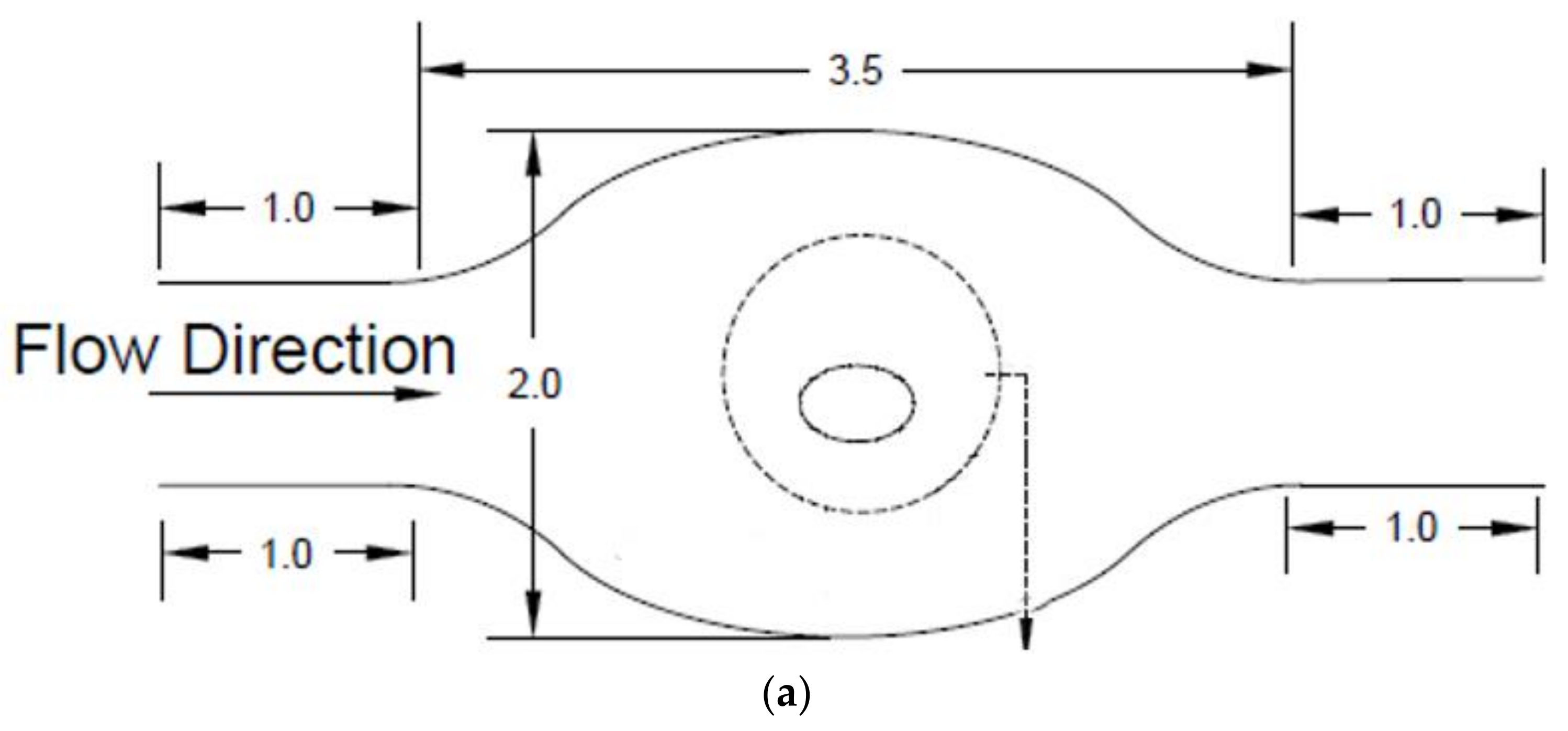
The mid-channel bar model is shown in Figure 2a. The measuring points are taken along the four different lines, i.e., 1, 2, 3, and 4 (Figure 2b).

The acoustic doppler velocimetry method is used to measure velocity (ADV). The ADV records the instantaneous value of velocity components at a relatively high frequency. The ADV measures velocity using the doppler shift principle. Researchers such as [27,28] discovered that when the sampling frequency increases, the noise in the signal also increases. Even after despiking of velocity data, part of the noise in the signal caused by the high sample frequency remains intrinsically in the signal [29]. The study by [30] conducted trials at various sampling rates and discovered that for a 10 MHz ADV, it is optimal to capture data at a sampling rate of 20 HZ to limit the likelihood of velocity ambiguities tainting the data. Researchers [31,32,33] have employed a sampling frequency of 20 Hz to analyze sweep/ejection events. Following this researcher’s informed advice based on their special first-hand experience with similar types of experiments, the sample frequency of 20 Hz was chosen for velocity measurement. Following [34], the data having correlation coefficients less than 70 are excluded from the measured velocity data. The uncertainty of acoustic doppler velocimetry reading is shown in

Table 2. The uncertainty in the ADV measurements.

Nominal Velocity Range (mm/s)	ADV Velocity Error (mm/s)
$\pm$50	$\pm$0.92
$\pm$100	$\pm$0.98
$\pm$200	$\pm$1.22

.

The velocity measurements are made at 16 different depths for each point. The relative depths at which velocity is measured for each point are shown in

Table 3. Relative depths at which velocities are measured for each point along the lines 1, 2, 3 and 4.

Relative Depth (z/h)
0.05
0.053
0.055
0.057
0.059
0.061
0.063
0.067
0.071
0.075
0.08
0.084
0.088
0.092
0.096
0.1

. Relative depth is the ratio of the distance from the bed (z) to the depth of the flow (h). The effect of bursting events is more predominant in the region closest to the wall [35]. Thus, the velocity measurements are taken in the region closest to the wall (z/h ≤ 0.1).

The experiments are performed in clear water conditions. On average, bedside shear stress is kept at a lower level than critical shear stress. This means that scouring takes place only when the local shear stress exceeds the critical shear stress. The mid-channel bar generates turbulence, which raises the local shear stress.

The bed elevation measurements are done:

(a)

Before the experiment begins;

(b)

When the experiment is over.

The difference between readings before and after the experiment is calculated; scouring is shown by a negative difference, and the depositional zone is indicated by a positive difference.

3. Analysis of Turbulent Kinetic Energy

The total turbulent kinetic energy ($Tke)$ is given by Equation (1).

$$\mathit{T}\mathit{k}\mathit{e}=\frac{\mathbf{1}}{\mathbf{2}}\left\{\overline{{\left({\mathit{u}}^{\prime }\right)}^2}+\overline{{\left({\mathit{v}}^{\prime }\right)}^2}+ \overline{{\left({\mathit{w}}^{\prime }\right)}^2}\right\}$$

(1)

The turbulent kinetic energy value for each individual direction is also computed. The turbulent kinetic energy for flow direction ($Tk{e}_x)$ is equal to $\frac{1}{2}\times \overline{{\left(u^{\prime }\right)}^2}$. Similarly, the turbulent kinetic energy for vertical direction ($Tk{e}_y)$ and transverse direction ($Tk{e}_z)$ are represented by $\frac{1}{2}\times \overline{{\left(v^{\prime }\right)}^2}$ and $\frac{1}{2}\times \overline{{\left(w^{\prime }\right)}^2},$respectively.

The flow direction is represented by the x notation in $Tk{e}_x$, the vertical direction is represented by the y notation in $Tk{e}_y$ and the transverse direction is represented by the z notation in $Tk{e}_z$. The x, y, and z notations are shown in Figure 2b.

The $u\prime$ represents the fluctuating velocity in the x (longitudinal flow) direction, $v\prime$ represents the fluctuating velocity in the y (vertical distance from bed) direction, and $w\prime$ represents the fluctuating velocity in the z (transverse) direction.

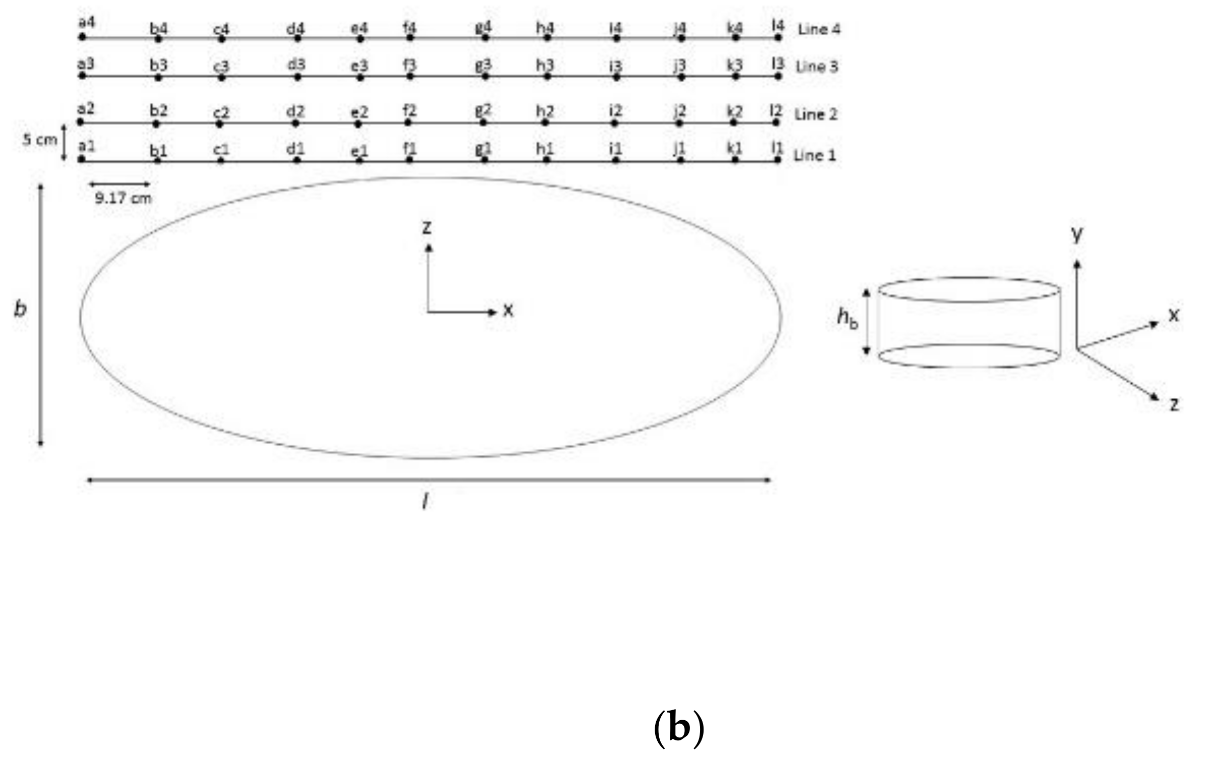
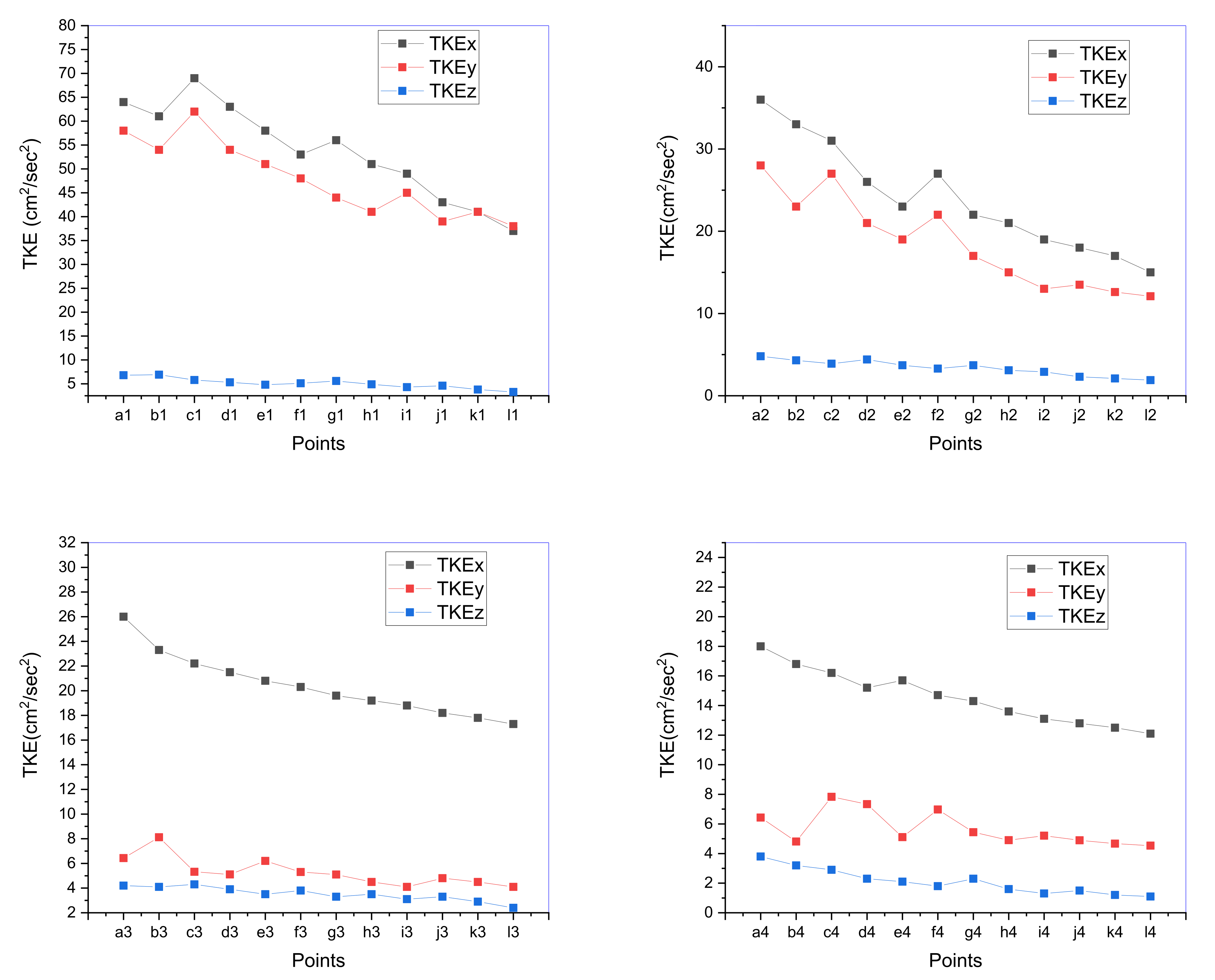
The turbulent kinetic energy ($Tke$) is depth-averaged for points in the near-bed region, as shown in Table 3. The near-bed depth-averaged values of the $Tke$ in all three directions (x, y, and z) are displayed in Figure 3 along four lines for the 1R experimental condition. Figure 3 shows that the $Tk{e}_x$ have the maximum value for all points plotted along four different lines. The vertical and transverse component of $Tke$ is negligible as compared to the longitudinal component ($Tk{e}_x)$.

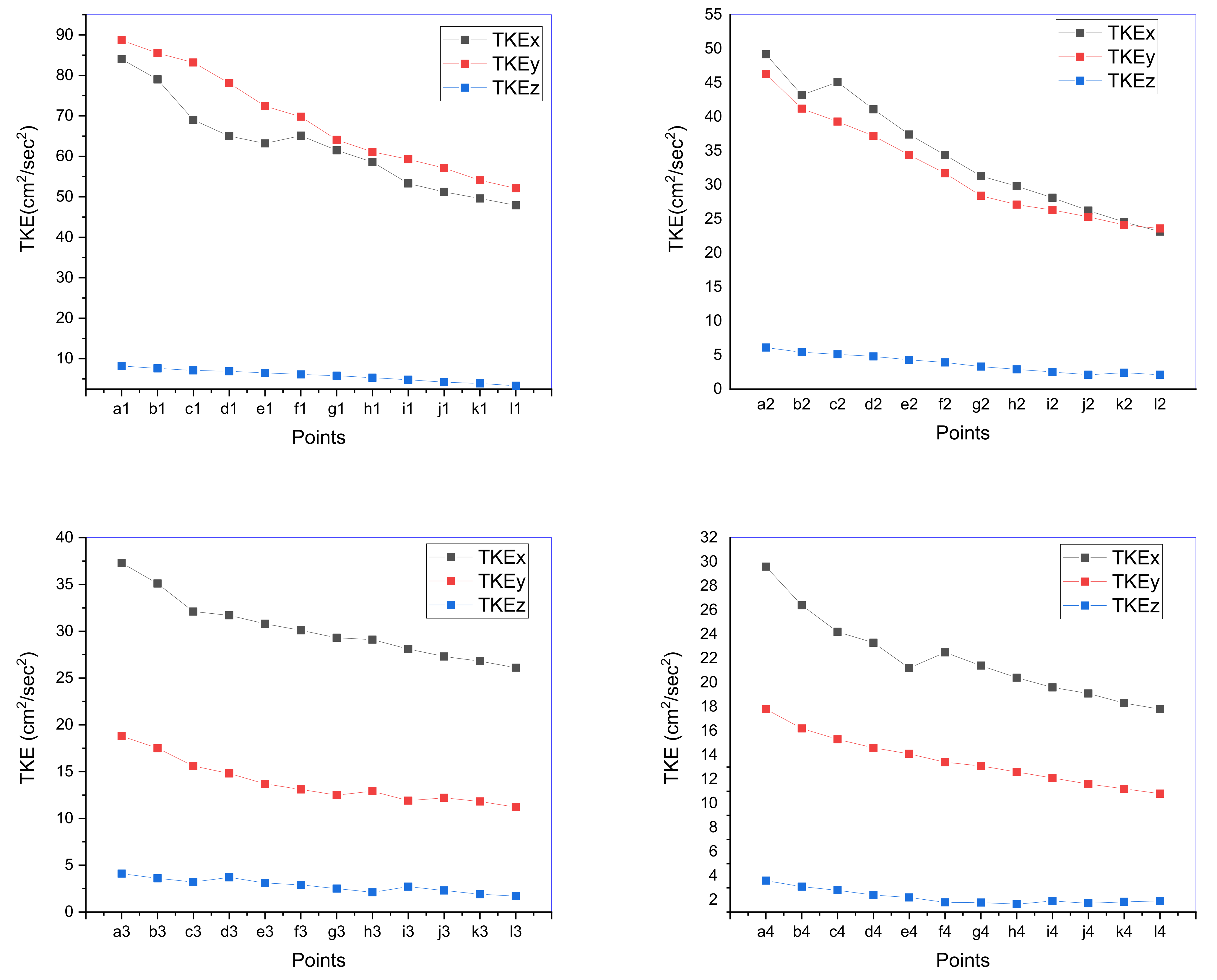
Figure 4 shows the depth-averaged $Tke$ component in all three directions (x, y, and z) along four lines for the 6R experimental condition. By comparing Figure 3 with Figure 4, it can be observed that the presence of a bar leads to the increase in the transverse component of turbulent kinetic energy$\left(Tk{e}_y\right)$. Along the lines 1 and 2, the value of $Tk{e}_y$ is significant, and its value is much greater compared to the $Tk{e}_z$ component (Figure 4). The value of $Tk{e}_y$ is more for points along the lines 1 and 2. In the other words, the effect of the bar mainly occurs along the lines located in the proximity of the bar. Similar results are also observed by [36,37,38].

Figure 5 shows the depth-averaged $Tke$ in all three directions (x, y, and z) along four lines for the 10R experimental condition. While comparing Figure 4 and Figure 5, it is observed that the magnitude of $Tk{e}_y$ increases with an increase in the submergence ratio. This indicates that the increase in submergence ratio leads to the transfer of turbulence in the transverse direction.

Figure 4 and Figure 5 shows that the magnitude of $Tk{e}_y$ is comparable to the $Tk{e}_x$ along the lines 1 and 2.

In most of the research, only the longitudinal and vertical velocity fluctuations are reckoned for bursting analysis. The above results show that the transverse flow component $Tk{e}_y$has a significant contribution to turbulence for points present in the proximity of the bar. This indicates that the transverse component cannot be neglected for analyzing the turbulence burst for bar configuration. Therefore, in the next section, the turbulence flow in the proximity of the bar is studied using the octant events.

4. Three-Dimensional Bursting Events

When studying the fully three-dimensional flow structure, quadrant analysis has limited utility [37,39,40,41]. For research on turbulent flow structure in a three-dimensional flow, octant events are used, which is more appropriate for 3D analysis. Octagonal bursting events depend on the sign of fluctuating longitudinal, vertical, and transverse velocity components, as per [41]. It enables us to fully consider the effects of secondary flow [37,39,40]. The 3D analysis of laboratory experiments would provide greater details regarding the sediment transport mechanism [37,42].

Based on fluctuating velocities, the turbulent bursts are divided into eight categories (

Table 4. Classification for three-dimensional octant bursting events.

Bursting Event Number (k)	Sign of Fluctuating Velocity			Octant Events	Zone
	${\mathit{u}}^{\prime }$	$\mathit{v}\prime$	$\mathit{w}\prime$
$P_1$	+	+	+	Internal outward interaction (I-A)
$P_2$	−	−	+	Internal ejection (II-A)	Zone A
$P_3$	−	−	−	Internal inward interaction (III-A)
$P_4$	+	+	−	Internal sweep (IV-A)
$P_5$	+	−	+	External outward interaction (I-B)
$P_6$	−	+	+	External ejection (II-B)	Zone B
$P_7$	−	+	−	External inward interaction (III-B)
$P_8$	+	−	−	External sweep (IV B)

). The occurrence probability of each octant event is determined by Equation (2) [41].

$${\mathit{P}}_{\mathit{k}}=\frac{{\mathit{n}}_{\mathit{k}}}{\mathit{N}}$$

(2)

$$\mathit{N}={\displaystyle \sum }_{\mathit{k}=\mathbf{1}}^{\mathbf{8}}{\mathit{n}}_{\mathit{k}}$$

(3)

Here, $P_k$ is the occurrence probability of an octant event that belongs to the octant k. $n_k$is the total number of octant events present in octant k, and N is the length of the velocity sample (Equation (3)). From Equation (2), the average occurrence probability of each octant event is computed.

The terminology for each of the eight $P_k$ events is adopted as per [41]. (Table 4). For instance, internal outward interaction (I-A) is named as$P_1$ (Table 4). The authors of [41] divided the bursting events into two zones, Zone A and Zone B (Table 4). $P_1$, $P_3,P_5,$ and $P_7$ are termed as odd events. Similarly, the $P_2$, $P_4,P_6,$ and $P_8$ events are termed as even events. The octant events $P_1$, $P_2$, $P_3,$ and $P_4$ lie in Zone A. The octant events $P_5$, $P_6$, $P_7,$ and $P_8$ lie in Zone B.

4.1. Three-Dimensional Transitional Movements Modelling

Bursting phenomena consist of quasi-organized and quasi-periodic events that occur randomly in turbulent flow [35]. These events have a spatio-temporal nature. Due to the significance of these transitional movements, they are modeled using the Markov chain process in the present study [41,43].

The bursting events can be modeled as continuous or discrete variables. As per [39,41,43], the octant events are considered discrete for modeling the transitional movements. The Markov chain process is most commonly used for modeling the time series of discrete variables. Thus, the Markov chain process is used herein for modeling the spatio-temporal transitional movements. The Markov chain represents a class of stochastic processes in which the future does not depend on the past; it depends on the present [44]. A stochastic process can be considered a Markov chain if the process consists of the Markovian properties that are needed to process the future. We require the information concerning the present state, and the past is independent of the process.

Bt represents the bursting event at time t. At any point in time, Bt can occur in any of the octants. The change in the current state of Bt with respect to time increment is defined as movement [43]. These movements have been modeled by [43] using the Markov chain process. The probability of these movements is defined as transition probability [39,41]. Schobesberger et al [41] modeled transition probability using zero-, first-, and second-order Markov chains. They observed that the first-order Markov chain is best for modeling the transition movements for rotational flow in the vortex chamber. In our study, there is no rotational flow, and thus the Markov chain order used by [41] cannot be used directly without proper investigation. Therefore, to find the best Markov chain order for present experimental datasets, the zero-, first-, and second-order Markov chains are analyzed using the Akaike information criterion and the Bayesian information criterion [44].

4.1.1. Zero-Order Markov Chain

The zero-order Markov chain denotes that the present condition is independent of the preceding condition, and it depends only on the current condition, as described by [45]. The probability for a zero-order Markov chain is computed by using Equation (4).

$${\mathit{p}}_{\mathit{i}}=\frac{{\mathit{n}}_{\mathit{i}}}{\mathit{N}}$$

(4)

Here,$n_i$ is the number of situations which belong to octant event $i,$ and $N$is the size of data.

The estimated occurrence of the transitional probability of the bursting process computed by using the zero-order Markov chain is shown by the following matrix.

0.088

0.171

0.145

0.081

0.135

0.187

0.122

0.071

4.1.2. First-Order Markov Chain

According to this concept, the probability of the next situation depends on the current situation, but it does not depend on the particular way that the model system arrived at the current situation [45]. The probability of first-order Markov chain transitional movements is calculated with the help of maximum likelihood estimates (Equation (5)).

$${\mathit{p}}_{\mathit{i}\mathit{j}} =\frac{{\mathit{n}}_{\mathit{i}\mathit{j}}}{{\mathit{n}}_{\mathit{i}}}$$

(5)

$${\mathit{n}}_{\mathit{i}}={\mathit{n}}_{\mathit{i}\mathbf{1}}+{\mathit{n}}_{\mathit{i}\mathbf{2}}+{\mathit{n}}_{\mathit{i}\mathbf{3}}+{\mathit{n}}_{\mathit{i}\mathbf{4}}+{\mathit{n}}_{\mathit{i}\mathbf{5}}+{\mathit{n}}_{\mathit{i}\mathbf{6}}+{\mathit{n}}_{\mathit{i}\mathbf{7}}+{\mathit{n}}_{\mathit{i}\mathbf{8}}$$

(6)

Here, $n_{ij}$ is the number of transitional movements from octant event $i$to octant event$j$. $n_i$ is the number of events belonging to octant $i$ at any instant (Equation (6)).

$p_{ij}$is movement probability from octant event $i$ at instant t to octant event $j$ at instant t+1.

By applying the first-order Markov Chain to the time series of octant events, the 64 elements of the transitional probability of first order can be observed.

$Matrix\left(A\right)$ is displaying the location of transitional movements obtained from the first-order Markov chain.

$$Matrix\left(A\right)=[\begin{array}{cccccccc}{p}_{1\to 1}& p_{1\to 2}& p_{1\to 3}& p_{1\to 4}& p_{1\to 5}& p_{1\to 6}& p_{1\to 7}& p_{1\to 8}\\ p_{2\to 1}& p_{2\to 2}& p_{2\to 3}& p_{2\to 4}& p_{2\to 5}& p_{2\to 6}& p_{2\to 7}& p_{2\to 8}\\ p_{3\to 1}& p_{3\to 2}& p_{3\to 3}& p_{3\to 4}& p_{3\to 5}& p_{3\to 6}& p_{3\to 7}& p_{3\to 8}\\ p_{4\to 1}& p_{4\to 2}& p_{4\to 3}& p_{4\to 4}& p_{4\to 5}& p_{4\to 6}& p_{4\to 7}& p_{4\to 8}\\ p_{5\to 1}& p_{5\to 2}& p_{5\to 3}& p_{5\to 4}& p_{5\to 5}& p_{5\to 6}& p_{5\to 7}& p_{5\to 8}\\ p_{6\to 1}& p_{6\to 2}& p_{6\to 3}& p_{6\to 4}& p_{6\to 5}& p_{6\to 6}& p_{6\to 7}& p_{6\to 8}\\ p_{7\to 1}& p_{7\to 2}& p_{7\to 3}& p_{7\to 4}& p_{7\to 5}& p_{7\to 6}& p_{7\to 7}& p_{7\to 8}\\ p_{8\to 1}& p_{8\to 2}& p_{8\to 3}& p_{8\to 4}& p_{8\to 5}& p_{8\to 6}& p_{8\to 7}& p_{8\to 8}\end{array}]$$

$p_{1\to 2}$ represents the probability of movement from octant $p_{1 }$ to octant $p_2$. Similarly, the remaining elements of the above matrix can be defined.

The estimated occurrence transitional probability of the bursting process computed by using the first-order Markov chain is shown by the matrix display below.

0.196	0.136	0.053	0.196	0.084	0.236	0.045	0.242
0.176	0.083	0.089	0.176	0.139	0.216	0.046	0.252
0.257	0.11	0.056	0.257	0.09	0.297	0.054	0.225
0.216	0.183	0.052	0.216	0.041	0.256	0.079	0.21
0.184	0.085	0.085	0.184	0.173	0.224	0.019	0.238
0.201	0.099	0.076	0.201	0.114	0.241	0.041	0.269
0.207	0.137	0.052	0.207	0.047	0.247	0.109	0.207
0.234	0.11	0.091	0.234	0.058	0.274	0.072	0.229

4.1.3. Second-Order Markov Chain

The second-order Markov chain is a stochastic process in which the probability of occurrence of present events at time t depends on the two preceding events at time t-1 and at time t-2. The probability is computed by a second-order Markov chain by using the conditional probability approach (Equation (7)).

$${\mathit{p}}_{\mathit{i}\mathit{j}\mathit{k}} =\frac{{\mathit{n}}_{\mathit{i}\mathit{j}\mathit{k}}}{{\mathit{n}}_{\mathit{i}\mathit{k}}}$$

(7)

$n_{ijk}$ is the number of $i$ events followed by$j$ events, then $j$ events followed by $k$ events.

$n_{ik}$ is the number of $i$ events followed by $k$ events.

By application of the second-order Markov chain, the 512 elements of transitional probability are computed.

The Transitional matrix computed by using the second-order Markov chain

0.157	0.126	0.093	0.028	0.14	0.174	0.062	0.22
0.214	0.05	0.003	0.015	0.177	0.039	0.134	0.368
0.211	0.211	0.003	0.034	0.103	0.138	0.074	0.226
0.221	0.207	0.029	0.033	0.085	0.161	0.071	0.193
0.201	0.083	0.046	0.037	0.24	0.156	0.014	0.223
0.204	0.132	0.105	0.051	0.072	0.133	0.052	0.251
0.165	0.181	0.023	0.099	0.038	0.228	0.038	0.228
0.271	0.101	0.035	0.053	0.042	0.192	0.103	0.203
0.262	0.151	0.071	0.061	0.172	0.055	0.03	0.308
0.216	0.05	0.136	0.181	0.107	0.026	0.048	0.236
0.194	0.05	0.037	0.159	0.181	0.146	0.014	0.219
0.338	0.338	0.03	0.159	0.037	0.011	0.037	0.05
0.207	0.059	0.09	0.153	0.182	0.044	0.003	0.262
0.149	0.087	0.054	0.052	0.148	0.119	0.054	0.337
0.232	0.117	0.075	0.082	0.152	0.15	0.075	0.117
0.266	0.097	0.168	0.043	0.092	0.047	0.021	0.266
0.339	0.092	0.038	0.057	0.09	0.163	0.012	0.209
0.234	0.123	0.071	0.061	0.127	0.106	0.071	0.207
0.328	0.116	0.081	0.081	0.051	0.101	0.005	0.237
0.144	0.082	0.168	0.047	0.043	0.141	0.21	0.165
0.186	0.096	0.072	0.05	0.173	0.097	0.039	0.287
0.238	0.08	0.095	0.076	0.135	0.042	0.008	0.326
0.259	0.118	0.023	0.052	0.054	0.15	0.148	0.196
0.28	0.091	0.12	0.068	0.057	0.047	0.131	0.206
0.307	0.194	0.009	0.015	0.022	0.145	0.083	0.225
0.316	0.111	0.031	0.148	0.103	0.007	0.03	0.254
0.254	0.111	0.127	0.053	0.055	0.091	0.055	0.254
0.255	0.194	0.006	0.02	0.052	0.15	0.037	0.286
0.175	0.202	0.014	0.032	0.068	0.158	0.095	0.256
0.287	0.118	0.038	0.044	0.038	0.176	0.064	0.235
0.262	0.17	0.071	0.024	0.016	0.198	0.071	0.188
0.285	0.183	0.052	0.015	0.031	0.139	0.082	0.213
0.236	0.102	0.073	0.036	0.135	0.109	0.022	0.287
0.063	0.063	0.146	0.121	0.169	0.252	0.146	0.04
0.109	0.099	0.099	0.045	0.109	0.133	0.089	0.317
0.094	0.202	0.122	0.032	0.014	0.455	0.041	0.04
0.063	0.069	0.088	0.057	0.198	0.112	0.175	0.238
0.115	0.065	0.06	0.08	0.198	0.238	0.204	0.04
0.207	0.082	0.043	0.068	0.106	0.098	0.168	0.228
0.094	0.134	0.067	0.045	0.108	0.364	0.148	0.04
0.129	0.137	0.041	0.045	0.073	0.196	0.121	0.258
0.102	0.086	0.083	0.174	0.237	0.133	0.145	0.04
0.148	0.083	0.032	0.048	0.118	0.384	0.147	0.04
0.125	0.167	0.059	0.047	0.03	0.389	0.143	0.04
0.111	0.089	0.118	0.059	0.167	0.282	0.134	0.04
0.113	0.109	0.088	0.067	0.128	0.105	0.175	0.215
0.184	0.174	0.073	0.067	0.022	0.325	0.115	0.04
0.164	0.086	0.089	0.026	0.076	0.119	0.151	0.289
0.147	0.183	0.055	0.029	0.067	0.329	0.15	0.04
0.165	0.134	0.148	0.068	0.085	0.056	0.21	0.134
0.151	0.17	0.053	0.079	0.016	0.327	0.164	0.04
0.18	0.215	0.048	0.04	0.005	0.09	0.171	0.251
0.118	0.06	0.038	0.025	0.176	0.348	0.195	0.04
0.111	0.132	0.103	0.046	0.093	0.127	0.144	0.244
0.27	0.109	0.006	0.051	0.075	0.328	0.121	0.04
0.147	0.131	0.125	0.046	0.034	0.129	0.183	0.205
0.123	0.136	0.05	0.037	0.037	0.367	0.21	0.04
0.151	0.077	0.053	0.116	0.053	0.069	0.182	0.299
0.158	0.087	0.055	0.046	0.078	0.375	0.161	0.04
0.175	0.175	0.027	0.016	0.05	0.119	0.14	0.298
0.103	0.087	0.11	0.06	0.125	0.358	0.117	0.04
0.138	0.085	0.054	0.046	0.083	0.085	0.19	0.319
0.172	0.13	0.085	0.054	0.023	0.348	0.148	0.04
0.136	0.103	0.102	0.061	0.043	0.111	0.162	0.282

For finding the best model for analyzing the stochastic nature of turbulent events, two different criteria are used (listed below):

• The Akaike information criterion (AIC);
• The Bayesian information criterion (BIC).

These criteria are based on the log-likelihood method [46].

The log-likelihood for zero-, first-, and second-order Markov chains are given by Equations (8)–(10), respectively.

$${\mathit{l}}_{\mathbf{0}}={\displaystyle \sum }_{\mathit{i}=\mathbf{1}}^{\mathit{i}=\mathbf{8}}{\mathit{n}}_{\mathit{i}}\mathbf{l}\mathbf{n}({\mathit{p}}_{\mathit{i}})$$

(8)

$${\mathit{l}}_{\mathbf{1}}={\displaystyle \sum }_{\mathit{j}=\mathbf{1}}^{\mathit{j}=\mathbf{8}}{\displaystyle \sum }_{\mathit{i}=\mathbf{1}}^{\mathit{i}=\mathbf{8}}{\mathit{n}}_{\mathit{i}\mathit{j}}\mathbf{l}\mathbf{n}({\mathit{p}}_{\mathit{i}\mathit{j}})$$

(9)

$${\mathit{l}}_{\mathbf{2}}={\displaystyle \sum }_{\mathit{k}=\mathbf{1}}^{\mathit{k}=\mathbf{8}}{\displaystyle \sum }_{\mathit{j}=\mathbf{1}}^{\mathit{j}=\mathbf{8}}{\displaystyle \sum }_{\mathit{i}=\mathbf{1}}^{\mathit{i}=\mathbf{8}}{\mathit{n}}_{\mathit{i}\mathit{j}\mathit{k}}\mathbf{l}\mathbf{n}({\mathit{p}}_{\mathit{i}\mathit{j}\mathit{k}})$$

(10)

The values of AIC and BIC are calculated using the equations given below (Equations (11) and (12)).

$$\mathrm{AIC}\left(\mathrm{m}\right)=-2*{\mathit{l}}_{\mathit{m}}+\mathbf{2}{\mathit{s}}^{\mathit{m}*\left(\mathit{s}-\mathbf{1}\right)}$$

(11)

$$\mathrm{BIC}\left(\mathrm{m}\right)=-2*{\mathit{l}}_{\mathit{m}}+\mathbf{2}{\mathit{s}}^{\mathit{m}*\left(\mathit{l}\mathit{n}\left(\mathit{n}\right)\right)}$$

(12)

In the above equation, s = 8, as it represents the eight bursting events. The value of order m that yields the lowest value in either Equation (11) or (12) is considered as the best Markov chain order for modeling the flow. The calculated values of AIC and BIC for the zero-, first-, and second-order Markov chains are displayed in

Table 5. AIC and BIC values for zero-, first-, and second-order Markov chains for present data set.

Criteria	Zero-Order Markov Chain	First-Order Markov Chain	Second-Order Markov Chain
AIC	18232	17752	18212
BIC	18210	17722	17866

. The first-order Markov chain process has the lowest values of AIC and BIC criteria. Therefore, the first-order Markov chain is used for studying the transitional movements of bursting events.

The transitional movements are divided into two main classes. The first class consists of movements that take place between the events that belong to the same zone, e.g., $p_{1\to 3}$ or $p_{2\to 4}$. The second class contains movements that occur between the events which belong to a different zone, e.g., $p_{1\to 6}$or $p_{8\to 3}$ [41]. The transitional movements that belong to the first class are called inner class movements. These inner class movements are further divided into three sub-classes mentioned below.

Stable movements: The event stays in the same octant as the time changes from t to t+1. These movements are located at the main diagonal of $Matrix\left(A\right)$, highlighted by bold letters. Examples include $p_{1\to 1}$ and $p_{8\to 8}$. These movements are further classified into Class A and Class B transitional movements based on their octant zone. Class A stable transitional movements are $p_{1\to 1}$, $p_{2\to 2}$, $p_{3\to 3}$, and $p_{4\to 4}$. Class B stable transitional movements are $p_{5\to 5}$, $p_{6\to 6}, p_{7\to 7}$, and$p_{8\to 8}$.

Marginal movements: The event moves to the neighboring event of the same zone as the time changes from t to t+1, e.g., $p_{3\to 4}$ and $p_{7\to 8}$.

Cross movements: The bursting events move to the cross events of the same zone as the time changes from t to t+1, e.g., $p_{2\to 4}$ and $p_{6\to 8}$.

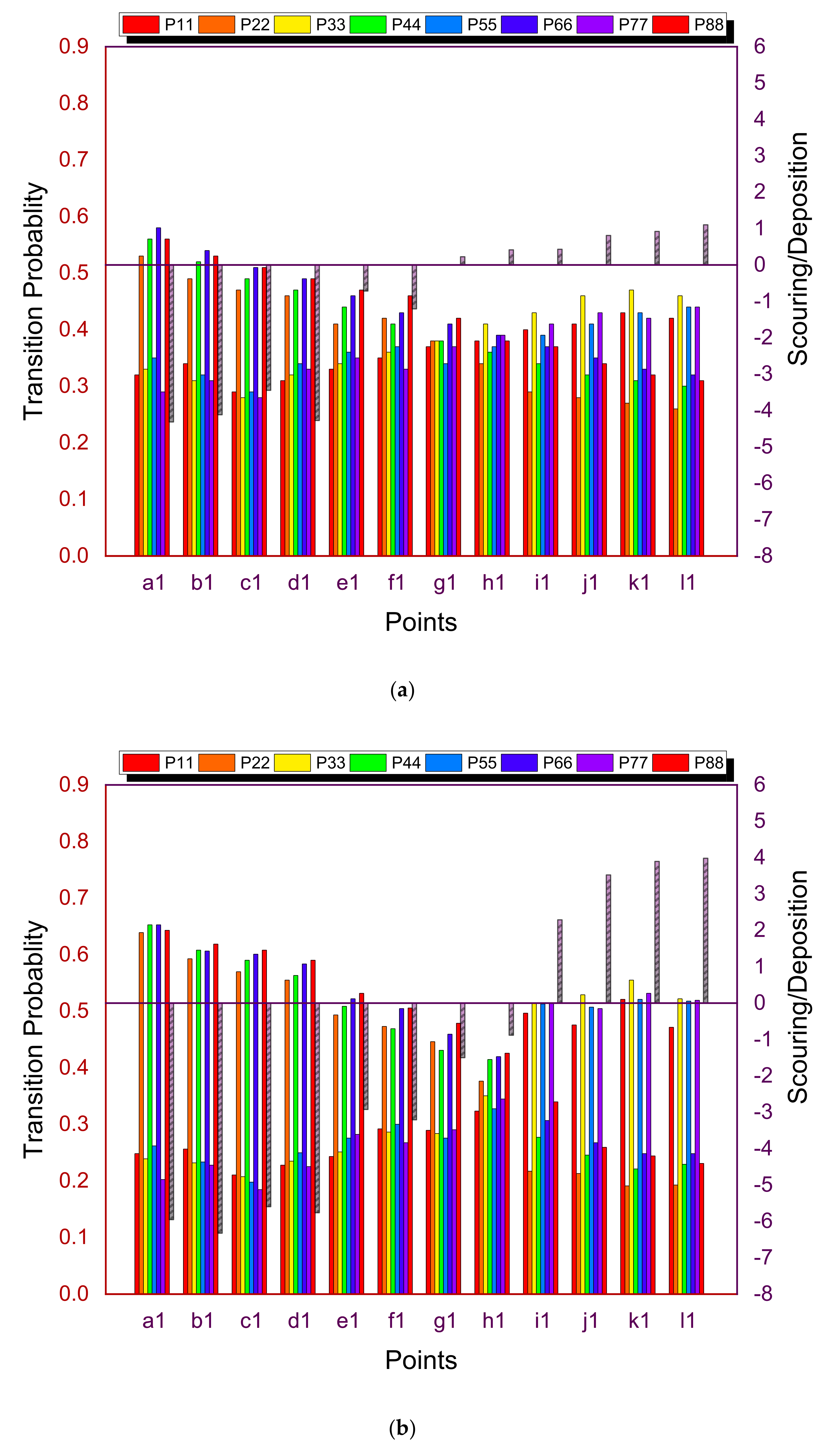
The transition probability of stable movements is depth-averaged for points in the near-bed region, as shown in Table 3. The near-bed depth-averaged values of transition probability of stable movements are plotted for 2R and 10R, respectively (Figure 6). The Primary Y axis in Figure 6 shows the values of near-bed depth-averaged stable transitional movements for twelve points along Line 1. The primary Y axis is shown on the left side of the vertical axis. All points cannot be displayed in Figure 6 for sake of clarity. As discussed in Section 3, the effect of turbulence generated due to the bar is maximum for points along Line 1. Therefore, only the points along Line 1 are plotted in Figure 6. The secondary Y axis in the Figure 6 is represented by the grey area, which depicts the scouring/deposition value observed at these twelve points. On the right side of the vertical axis lies the secondary Y axis. A negative value in the secondary y axis indicates scouring, while a positive value in the secondary y axis indicates the depositional zone.

By comparing the primary and secondary Y axis of Figure 6, it was found that the higher values of $p_{2\to 2}$, $p_{4\to 4}$, $p_{6\to 6}$, and $p_{8\to 8}$were observed at scouring points and higher values of $p_{1\to 1}$, $p_{3\to 3}$, $p_{5\to 5}$, $p_{7\to 7}$ observed at depositional points. This suggests that the odd stable movements are due to deposition, whereas the even stable movements are due to scouring in the vicinity of the bar. As the submergence ratio rises, the level of scouring rises as well (Figure 6). The value of $p_{2\to 2}$, $p_{4\to 4}$, $p_{6\to 6}$, and $p_{8\to 8}$ also rises as the submergence ratio for scouring locations rises (Figure 6).

The work by [41] analyzed the stable transitional movements. However, they did not propose a parameter that summarized the effect of stable transition movements into one parameter. In the present study, the new parameter transition ratio (TR) is proposed (Equation (13)). This parameter takes into account the effect of stable transition movements on the local streambed elevation change occurring in the proximity of the bar.

It is the ratio of summation of odd stable movement to the summation of even stable movement (Equation (13)).

$$\mathrm{TR}=\frac{{\mathit{p}}_{\mathbf{1}\to \mathbf{1}}+{\mathit{p}}_{\mathbf{3}\to \mathbf{3}}+{\mathit{p}}_{\mathbf{5}\to \mathbf{5}}+{\mathit{p}}_{\mathbf{7}\to \mathbf{7}} }{{\mathit{p}}_{\mathbf{2}\to \mathbf{2}}+{\mathit{p}}_{\mathbf{4}\to \mathbf{4}}+{\mathit{p}}_{\mathbf{6}\to \mathbf{6}}+{\mathit{p}}_{\mathbf{8}\to \mathbf{8}} }$$

(13)

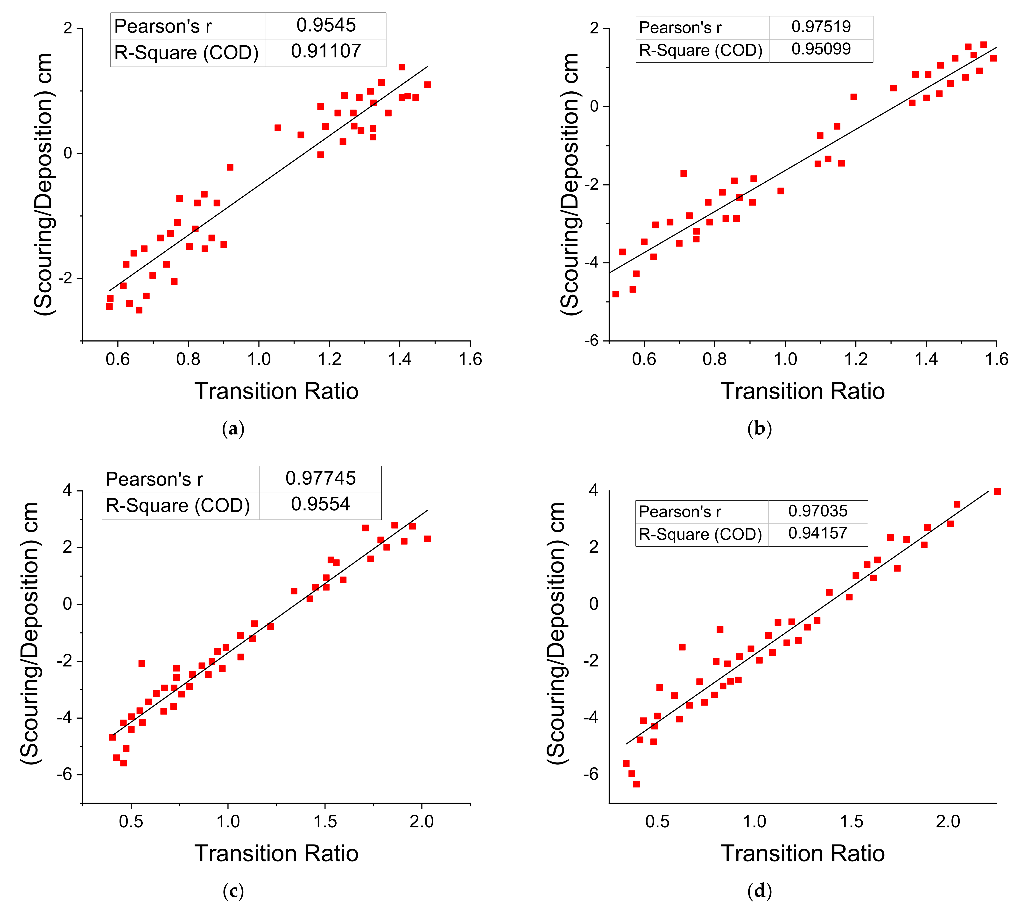
Figure 7 shows the plot of the parameter transition ratio against the scouring/deposition observed at measuring points for 2R, 6R, 8R, and 10R experimental runs.

Figure 7 highlights the predominance of the linear relationship of transition ratio with the scouring/deposition data. For all tests performed, the coefficient of determination and Pearson R value are greater than 0.9.

The results indicate that only the stable transition movements are associated with the variation in elevation of bed detected in the proximity of the bar. It is known that the sum of probabilities is equal to one. Thus, a change in the probability of one stable movement will cause changes in the other stable movements. Therefore, we have modeled a relationship between these stable movements for our experimental dataset. By utilizing statistical analysis, it has been observed that the best mathematical relationships would be developed if the Class A and Class B transition movements were modeled separately (

Table 6. Mathematical relationships for Class A and Class B stable transition movements for present data set.

Transition Movements	Mathematical Equations	Determination Coefficient (R2)
Class A Transition Movement	$P_{1\to 1}=-2.52*P_{2\to 2}^{3.27}$$+0.93*P_{3\to 3}^{1.14}+1.42*P_{4\to 4}^{2.42}$	0.95
	$P_{2\to 2}=-0.58*P_{1\to 1}^{0.44}$$+0.51*P_{3\to 3}^{0.54}+0.98*P_{4\to 4}^{0.87}$	0.94
	$P_{3\to 3}=0.99*P_{1\to 1}^{0.88}$$-0.28*P_{2\to 2}^{-0.71}+0.24*P_{4\to 4}^{-0.87}$	0.93
	$P_{4\to 4}=-0.66*P_{1\to 1}^{0.46}$$+1.04*P_{2\to 2}^{1.18}-0.57*P_{3\to 3}^{0.57}$	0.95
Class B Transition Movement	$P_{5\to 5}=-1.94*P_{6\to 6}^{3.27}$$+0.91*P_{7\to 7}^{1.21}+1.22*P_{8\to 8}^{2.12}$	0.92
	$P_{6\to 6}=-0.08*P_{5\to 5}^{-0.13}$$-0.02*P_{7\to 7}^{3.84}+0.85*P_{8\to 8}^{1.17}$	0.93
	$P_{7\to 7}=1.2*P_{5\to 5}^{0.97}$$-0.37*P_{6\to 6}^{-0.81}+0.32*P_{8\to 8}^{-0.95}$	0.90
	$P_{8\to 8}=-0.78*P_{5\to 5}^{0.58}$$+1.14*P_{6\to 6}^{1.29}-0.69*P_{7\to 7}^{0.68}$	0.93

). The high values of correlation for these expressions indicate that they are correctly predicting the relationship between the stable movements. In the future, the above equations can be elaborated after validating them with the other researchers’ datasets.

5. Temporal Structure of Octant Events

Most of the researchers, such as [47,48], have analyzed the residence time vs. frequency graph of quadrant events to study the temporal behaviors of bursting events. Very few researchers have studied the residence time vs. frequency graph for octant events [24,49]. Due to the close relationship of stable transitional movements with the bed elevation changes, the temporal behavior of stable transitional movements of octant events has been analyzed, which is presented in this study. As per our knowledge, the residence time–frequency relationship for transitional movements is not studied yet by any researcher.

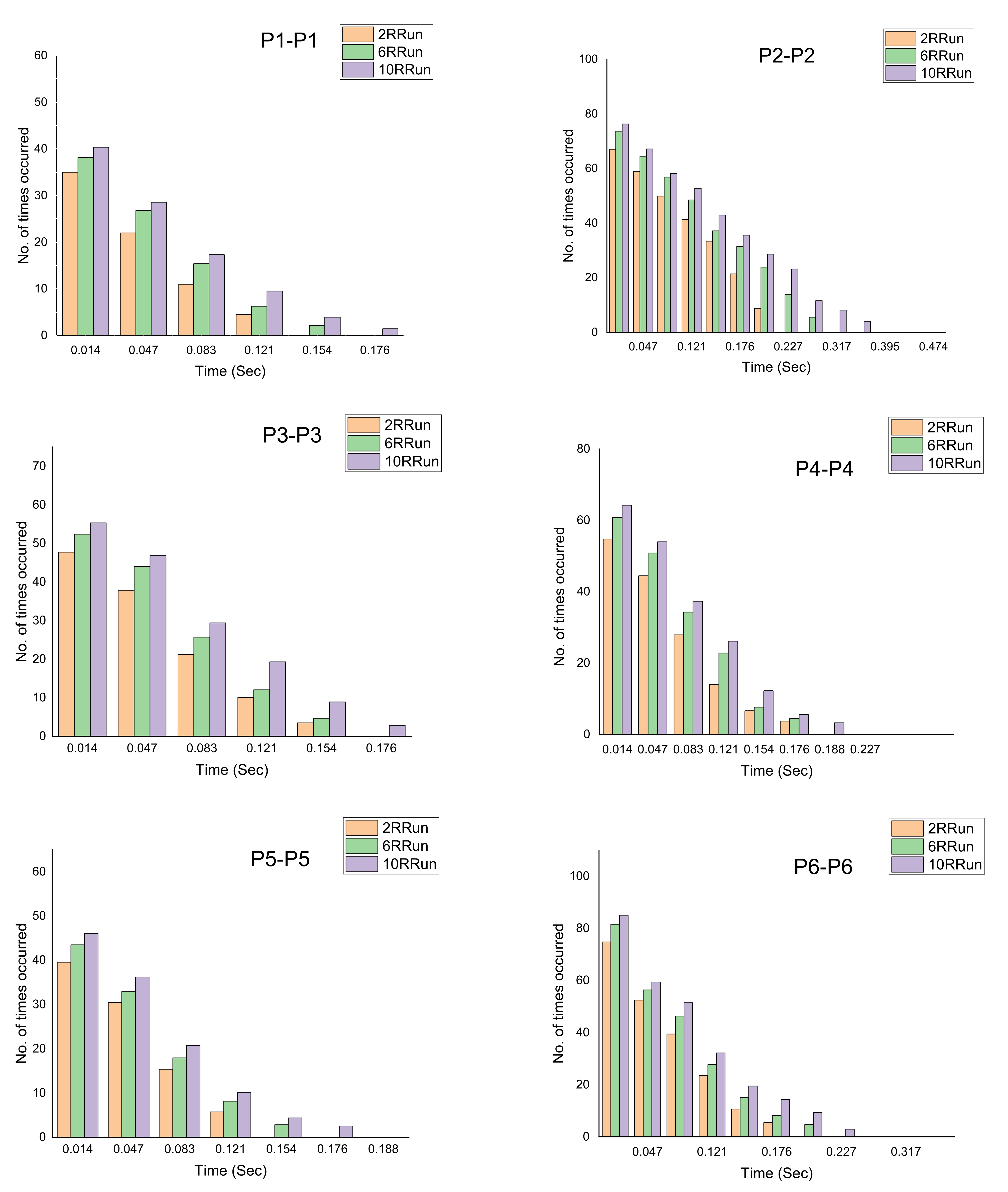
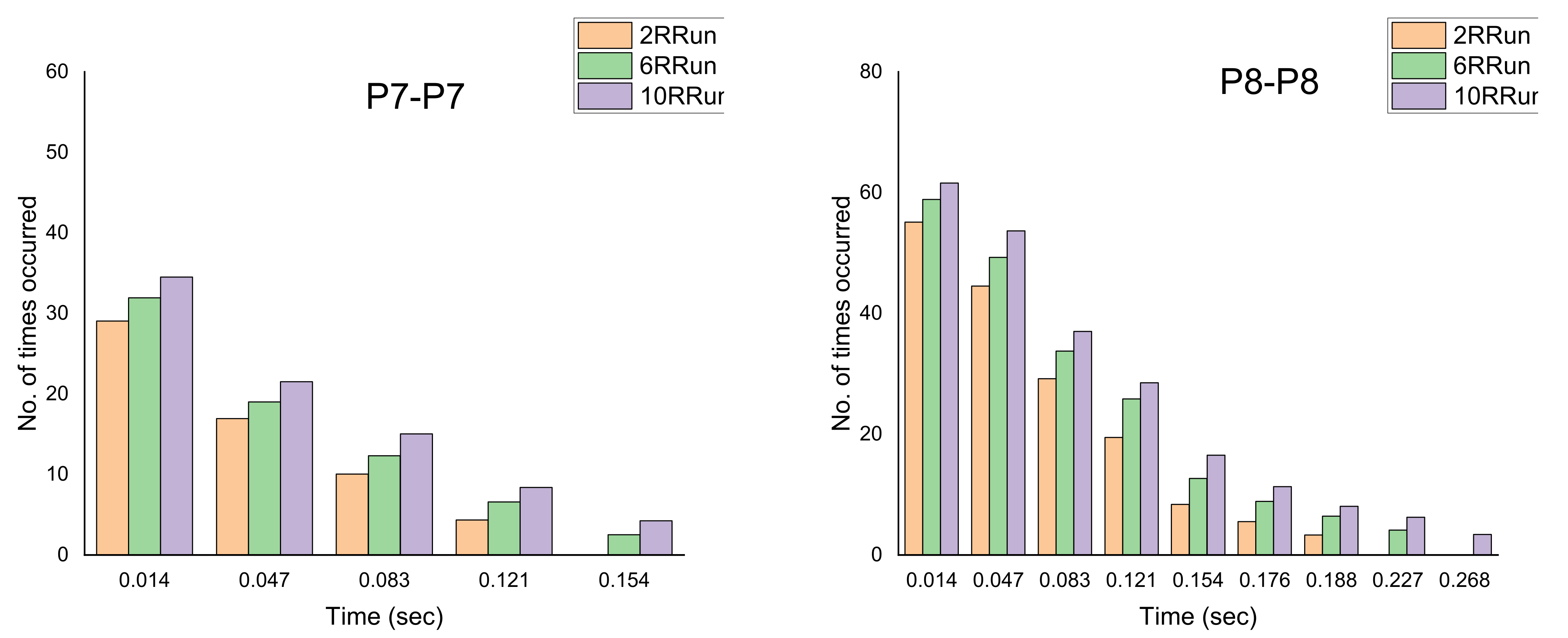
The histogram of residence time vs. frequency graph for stable transitional movement is plotted and analyzed for scouring as well as for depositional regions. The residence time of stable transitional movement is computed by counting the number of times particular movements occurred in a succession$n_{i,k}$ multiplied by the $\mathrm{\Delta }t$(inverse of sampling frequency). In our experiments, the sampling frequency of velocity measurement is 20 Hz.

Figure 8 shows the histogram of residence time vs. frequency graph for stable transitional movements of octant events averaged for scouring points in the proximity of the mid-channel bar. It is clear from Figure 8 that the $p_{2\to 2}$, $p_{4\to 4}$, $p_{6\to 6}$, and $p_{8\to 8}$ transitional movements are particularly persistent for the scouring region. This indicates that the ‘even’ stable transitional movements are temporally more stable as compared to the ‘odd’ stable transitional movement at the scouring region. The maximum period of 0.4 s is observed for $p_{2\to 2}$ movement. The persistence of ‘even’ stable transitional movement further increases with an increase in the submergence ratio (Figure 8).

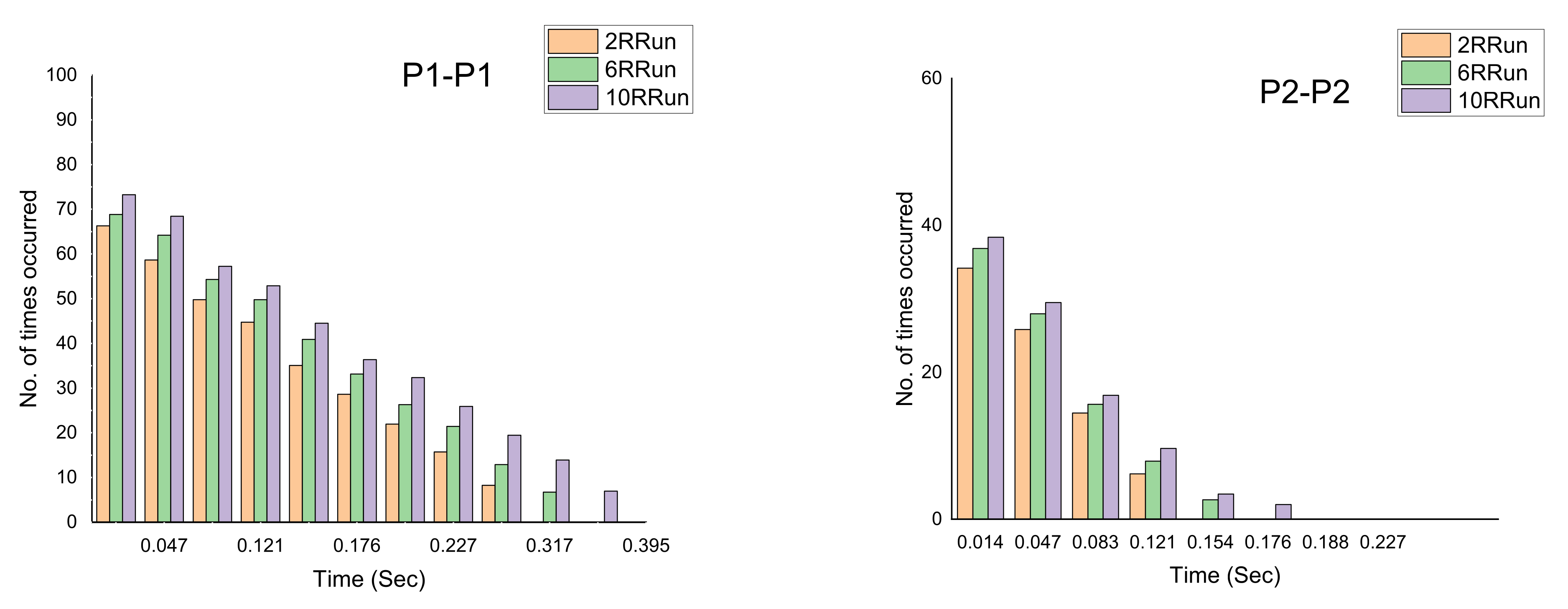
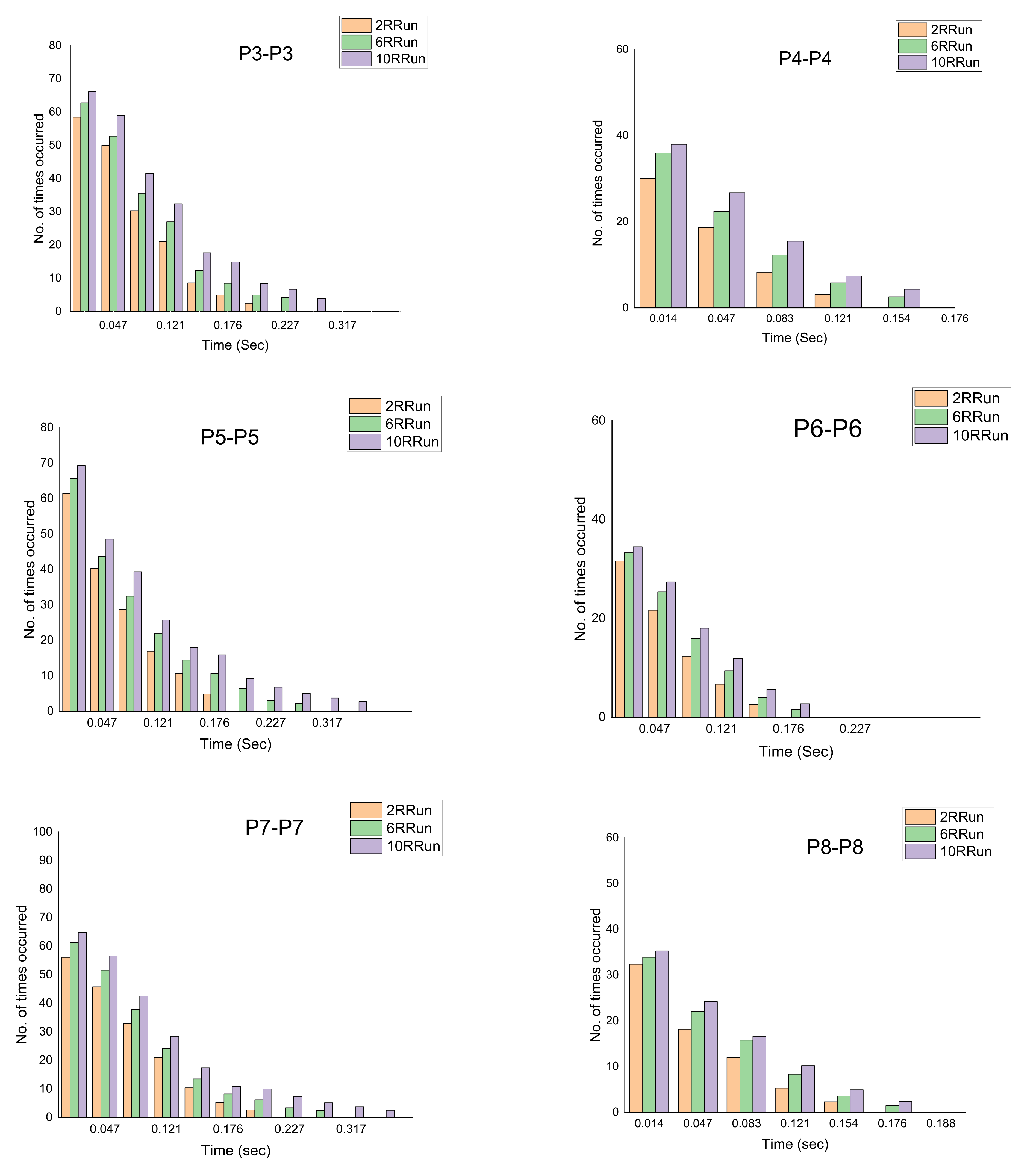
Figure 9 below shows the histogram of residence time vs. frequency graph for stable transitional movements averaged for depositional points in the proximity of the bar. The ‘odd’ stable transitional movements are particularly persistent for the depositional region. In Section 4.1, the results show that the transitional probability of stable movements is linked with the bed level changes observed. In addition, this section indicates that the temporal behavior of stable movements also has a link with the scouring/depositional regions. The temporal behavior of stable transitional movements has probably been analyzed for the first time to date in this study. These research outcomes can be further elaborated for analyzing scour and deposition phenomena in real-life water management projects in the future.

5.1. Criticality of Transverse TKE around Mid-Channel Bar

The data analysis using the octant events approach shows that the magnitude of transverse turbulent kinetic energy, $Tk{e}_y$, is comparable to the longitudinal turbulent kinetic energy, $Tk{e}_x$, in addition to vertical turbulent energy.

In most of the research adopting the quadrant events approach, only the longitudinal and vertical velocity fluctuations are reckoned with for bursting analysis. The present results show that the transverse flow component $Tk{e}_y$has a significant contribution to turbulence for points present in the proximity of the bar. This indicates that the transverse component cannot be ignored in analyzing the turbulence burst analysis for mid-channel bar configuration. Therefore, in this study on the mid-channel bar, the turbulence flow structure in the proximity of the bar is analyzed using the octant events approach. Furthermore, from the processing of the experimental results of octant turbulent events, it could also be discerned that the magnitude of the transverse bursting component increases with an increase in the submergence ratio. This indicates that the increase in submergence ratio leads to the transfer of turbulence in the transverse direction.

5.2. Analysis of 3D TKE Bursts Data for Development of New Transition Ratio Parameter

The octant events used in this research on the turbulent flow structure in three-dimensional flow around the mid-channel bar proved to be more appropriate for 3D analysis. The octagonal bursting events depend on the sign of fluctuating longitudinal, vertical, and transverse velocity components. It enables us to fully consider the effects of secondary flow by considering all three components.

For modeling the transitional movements, the octant events are considered discrete. The Markov chain process is most commonly used for modeling the time series of discrete variables. Thus, the Markov chain process is used herein for modeling the spatial and temporal transitional movements.

For finding the best Markov chain order for present experimental datasets, the zero-, first-, and second-order Markov chains are analyzed using the Akaike information criterion and the Bayesian information criterion. The first-order Markov chain process has yielded the lowest values of the AIC and BIC criteria. Therefore, the first-order Markov chain is used for studying the transitional movements of bursting events.

Keshavarzi et al [40] had analyzed the stable transitional movements, but they had not proposed a parameter that could sum up the effect of stable transition movements into a single parameter. In the present study, a new parameter transition ratio (TR) is proposed (Equation 13). The Transition Ratio takes into account the effect of stable transition movements on the local streambed elevation change occurring in the proximity of the mid-channel bar. The newly proposed parameter, the Transition Ratio, in this research has evolved as a quantitative measure of the turbulent bursting effect on the streambed elevation changes due to erosion and/or deposition.

Another notable outcome of the present research shows that the transitional probability of stable movements has a relationship with the bed level changes. Furthermore, the temporal behavior of stable movements also has a link with the scouring and depositional zones. Probably for the first time in this study, the temporal behavior of stable transitional movements has been analyzed.

Given considerable prospects of gainful practical applications, these research outcomes warrant further elaboration in the future for assessing scour and deposition processes in real-world water management projects.

6. Conclusions

The following conclusions emerged from the current study’s experimental data analysis:

• A key finding yielded from the present research highlights that the transverse component of the turbulent burst phenomenon has a significant contribution to turbulence generation for points present in close proximity to the bar. This indicates that the transverse component cannot be ignored while analyzing the turbulent burst analysis of fluvial situations with a braid bar when 3D kinetic forces predominate. The results also indicate that the increase in submergence ratio due to the heightened bar leads to the transfer of an appreciable quantum of turbulence in the transverse direction.
• The Bayesian information and the Akaike information criteria are used to examine the zero-, first-, and second-order Markov chains in order to determine the appropriate Markov chain order for the current experimental datasets. The AIC and BIC criterion for the first-order Markov chain process are the lowest. As a result, for investigating the transitional movements of bursting events, the first-order Markov chain is used.
• A new parameter has been added in this study: the transition ratio, which has been developed to depict the relationship between streambed elevation changes and steady transitional movements of 3D turbulent bursts using octant events. The results succinctly portrayed that the transition ratio is influenced greatly by changes in stream bed elevation, making it an appropriate parameter for studying scour and deposition events in real-world water management projects.
• Relationships between stable movements are modeled in this study. The high values of correlation for these expressions indicate that they are correctly predicting the relationship between the stable movements in our experimental dataset. The above relationships can be elaborated on in future studies after validation with the datasets of other research workers.
• For better understanding the temporal behavior of stable transitional movements, the residence time vs. frequency graphs are plotted for scouring as well as for depositional regions. The results show that the ‘even’ movements are particularly persistent in the scouring region and the ‘odd’ stable transitional movements are particularly related to the depositional region. The temporal behavior of stable transitional movements for octant events has been analyzed, probably for the first time, in this study.

References

- Ashmore, P.E. Laboratory modelling of gravel braided stream morphology. Earth Surf. Process. Landf. 1982, 7, 201–225. [Google Scholar] [CrossRef]
- Ashworth, P.; Ferguson, R.; Powell, M. Bedload Transport and Sorting in Braided Channels. In Dynamics of Gravel-Bed; Billi, R.D., Hey, C.R., Thorne, P., Eds.; John Wiley and Sons: New York, NY, USA, 1992; pp. 497–515. [Google Scholar]
- Ashworth, P. Mid-channel bar growth and its relationship to local flow strength and direction. Earth Surf. Process. Landf. 1996, 21, 103–123. [Google Scholar] [CrossRef]
- Best, J.; Ashworth, P.; Bristow, C.S.; Roden, J.E. Three-Dimensional Sedimentary Architecture of a Large, Mid-Channel Sand Braid Bar, Jamuna River, Bangladesh. J. Sediment. Res. 2003, 73, 516–530. [Google Scholar] [CrossRef]
- Jang, C.-L.; Shimizu, Y. Vegetation effects on the morphological behavior of alluvial channels. J. Hydraul. Res. 2007, 45, 763–772. [Google Scholar] [CrossRef]
- Ashworth, P.J.; Best, J.L.; Roden, J.E.; Bristow, C.S.; Klaassen, G.J. Morphological evolution and dynamics of a large, sand braid-bar, Jamuna River, Bangladesh. Sedimentol. 2000, 47, 533–555. [Google Scholar] [CrossRef]
- Khan, A.M.; Sharma, N.; Singhal, G.D. Experimental study on bursting events around a bar in physical model of a braided channel. ISH J. Hydraul. Eng. 2017, 23, 63–70. [Google Scholar] [CrossRef]
- Khan, M.A.; Sharma, N. Investigation of Coherent Flow Turbulence in the Proximity of Mid-Channel Bar. KSCE J. Civ. Eng. 2019, 23, 5098–5108. [Google Scholar] [CrossRef]
- Ashmore, P.; Parker, G. Confluence scour in coarse braided streams. Water Resour. Res. 1983, 19, 392–402. [Google Scholar] [CrossRef] [Green Version]
- Nakagawa, H.; Nezu, I. Bursting phenomenon near the wall in open-channel flows and its simple mathematical model. Kyoto Univ. Fac. Eng. Mem. 1978, 40, 213–240. [Google Scholar]
- Nakagawa, H.; Nezu, I. Structure of space-time correlations of bursting phenomena in an open-channel flow. J. Fluid Mech. 1981, 104, 1–43. [Google Scholar] [CrossRef]
- Salim, S.; Pattiaratchi, C.; Tinoco, R.; Coco, G.; Hetzel, Y.; Wijeratne, S.; Jayaratne, R. The influence of turbulent bursting on sediment resuspension under unidirectional currents. Earth Surf. Dyn. 2017, 5, 399–415. [Google Scholar] [CrossRef] [Green Version]
- Khan, M.A.; Sharma, N. Turbulence Study Around Bar in a Braided River Model. Water Resour. 2019, 46, 353–366. [Google Scholar] [CrossRef]
- Heathershaw, A.D.; Thorne, P.D. Sea-bed noises reveal role of turbulent bursting phenomenon in sediment transport by tidal currents. Nature 1985, 316, 339–342. [Google Scholar] [CrossRef]
- Nelson, J.M.; Shreve, R.L.; McLean, S.R.; Drake, T.G. Role of Near-Bed Turbulence Structure in Bed Load Transport and Bed Form Mechanics. Water Resour. Res. 1995, 31, 2071–2086. [Google Scholar] [CrossRef]
- Detert, M.; Weitbrecht, V.; Jirka, G. Simultaneous Velocity and Pressure Measurements Using PIV and Multi Layer Pressure Sensor Arrays in Gravel Bed Flows; HMEM: Lake Placid, NY, USA, 2007. [Google Scholar]
- Khan, M.A.; Sharma, N. Analysis of turbulent flow characteristics around bar using the conditional bursting technique for varying discharge conditions. KSCE J. Civ. Eng. 2018, 22, 2315–2324. [Google Scholar] [CrossRef]
- Hardy, R.J.; Lane, S.N.; Ferguson, R.; Parsons, D. Emergence of coherent flow structures over a gravel surface: A numerical experiment. Water Resour. Res. 2007, 43. [Google Scholar] [CrossRef] [Green Version]
- Keylock, C. Identifying linear and non-linear behaviour in reduced complexity modelling output using surrogate data methods. Geomorphology 2007, 90, 356–366. [Google Scholar] [CrossRef]
- Paik, J.; Escauriaza, C.; Sotiropoulos, F. Coherent Structure Dynamics in Turbulent Flows Past In-Stream Structures: Some Insights Gained via Numerical Simulation. J. Hydraul. Eng. 2010, 136, 981–993. [Google Scholar] [CrossRef]
- Keylock, C.J.; Tokyay, T.; Constantinescu, G. A method for characterising the sensitivity of turbulent flow fields to the structure of inlet turbulence. J. Turbul. 2011, 12, N45. [Google Scholar] [CrossRef]
- Best, J.L.; Ashworth, P.J.; Sarker, M.H.; Roden, J.E. The Brahmaputra-Jamuna River, Bangladesh. In Large Rivers; Wiley: Hoboken, NJ, USA, 2007; pp. 395–433. [Google Scholar]
- Ölçmen, S.M.; Simpson, R.L.; Newby, J.W. Octant analysis based structural relations for three-dimensional turbulent boundary layers. Phys. Fluids 2006, 18, 025106. [Google Scholar] [CrossRef] [Green Version]
- Keylock, C.J.; Lane, S.N.; Richards, K.S. Quadrant/octant sequencing and the role of coherent structures in bed load sediment entrainment. J. Geophys. Res. Earth Surf. 2014, 119, 264–286. [Google Scholar] [CrossRef]
- Nagano, Y.; Tagawa, M. A structural turbulence model for triple products of velocity and scalar. J. Fluid Mech. 1990, 215, 639–657. [Google Scholar] [CrossRef]
- Madden, M.M., Jr. Octant Analysis of the Reynolds Stresses in the Three Dimensional Turbulent Boundary Layer of a Prolate Spheroid. Doctoral Dissertation, Virginia Tech, Blacksburg, VA, USA, 1997. [Google Scholar]
- Voulgaris, G.; Trowbridge, J.H. Evaluation of the acoustic Doppler velocimeter (ADV) for turbulence measurements. J. Atmos. Ocean. Technol. 1998, 15, 272–289. [Google Scholar] [CrossRef] [Green Version]
- McLelland, S.J.; Nicholas, A.P. A new method for evaluating errors in high-frequency ADV measurements. Hydrol. Processes 2000, 14, 351–366. [Google Scholar] [CrossRef]
- Mori, N.; Suzuki, T.; Kakuno, S. Noise of Acoustic Doppler Velocimeter Data in Bubbly Flows. J. Eng. Mech. 2007, 133, 122–125. [Google Scholar] [CrossRef]
- Wahl, T.L. Analyzing ADV Data Using WinADV. In Building Partnerships; American Society of Civil Engineers (ASCE): Location, UK, 2000; pp. 1–10. [Google Scholar]
- Schindler, R.J.; Robert, A. Flow and turbulence structure across the ripple-dune transition: An experiment under mobile bed conditions. Sedimentology 2005, 52, 627–649. [Google Scholar] [CrossRef]
- Duan, J.G.; He, L.; Fu, X.; Wang, Q. Mean flow and turbulence around experimental spur dike. Adv. Water Resour. 2009, 32, 1717–1725. [Google Scholar] [CrossRef]
- Duan, J.; He, L.; Wang, G.; Fu, X. Turbulent burst around experimental spur dike. Int. J. Sediment Res. 2011, 26, 471–523. [Google Scholar] [CrossRef]
- Goring, D.G.; Nikora, V.I. Despiking Acoustic Doppler Velocimeter Data. J. Hydraul. Eng. 2002, 128, 117–126. [Google Scholar] [CrossRef] [Green Version]
- Kline, S.; Reynolds, W.; Schraub, F.; Runstadler, P. The structure of turbulent boundary layers. J. Fluid Mech. 1967, 30, 741–773. [Google Scholar] [CrossRef] [Green Version]
- Kumar, A.; Kothyari, U.C. Three-Dimensional Flow Characteristics within the Scour Hole around Circular Uniform and Compound Piers. J. Hydraul. Eng. 2012, 138, 420–429. [Google Scholar] [CrossRef]
- Keshavarzi, A.; Melville, B.; Ball, J. Three-dimensional analysis of coherent turbulent flow structure around a single circular bridge pier. Environ. Fluid Mech. 2014, 14, 821–847. [Google Scholar] [CrossRef]
- Vijayasree, B.A.; Eldho, T.I.; Mazumder, B.S. Turbulence statistics of flow causing scour around circular and oblong piers. J. Hydraul. Res. 2019, 58, 673–686. [Google Scholar] [CrossRef]
- Keshavarzi, A.; Gheisi, A. Three-dimensional fractal scaling of bursting events and their transition probability near the bed of vortex chamber. Chaos Solitons Fractals 2007, 33, 342–357. [Google Scholar] [CrossRef]
- Keshavarzi, A.R.; Gheisi, A.R. Stochastic nature of three dimensional bursting events and sediment entrainment in vortex chamber. Stoch. Hydrol. Hydraul. 2006, 21, 75–87. [Google Scholar] [CrossRef]
- Schobesberger, J.; Lichtneger, P.; Hauer, C.; Habersack, H.; Sindelar, C. Three-Dimensional Coherent Flow Structures during Incipient Particle Motion. J. Hydraul. Eng. 2020, 146, 04020027. [Google Scholar] [CrossRef]
- Smith, H.D.; Foster, D.L. Three-Dimensional Flow around a Bottom-Mounted Short Cylinder. J. Hydraul. Eng. 2007, 133, 534–544. [Google Scholar] [CrossRef]
- Gheisi, A.R.; Alavimoghaddam, M.R.; Dadrasmoghaddam, A. Markovian–Octant analysis based stable turbulent shear stresses in near-bed bursting phenomena of vortex settling chamber. Environ. Fluid Mech. 2006, 6, 549–572. [Google Scholar] [CrossRef]
- Tong, H. Determination of the order of a Markov chain by Akaike’s information criterion. J. Appl. Probab. 1975, 12, 488–497. [Google Scholar] [CrossRef]
- Gilks, W.R.; Richardson, S.; Spiegelhalter, D. Markov Chain Monte Carlo in Practice; CRC Press: Boca Raton, FL, USA, 1995. [Google Scholar]
- Akaike, H. A new look at the statistical model identification. IEEE Trans. Autom. Control 1974, 19, 716–723. [Google Scholar] [CrossRef]
- Metzger, M.; McKeon, B.; Arce-Larreta, E. Scaling the characteristic time of the bursting process in the turbulent boundary layer. Phys. D Nonlinear Phenom. 2010, 239, 1296–1304. [Google Scholar] [CrossRef]
- Tang, Z.; Jiang, N.; Zheng, X.; Wu, Y. Bursting process of large- and small-scale structures in turbulent boundary layer perturbed by a cylinder roughness element. Exp. Fluids 2016, 57, 1–14. [Google Scholar] [CrossRef]
- Khan, M.A. Experimental Study on Turbulence in the Vicinity of Mid-Channel Bar of Braided River Reach. Ph.D. Thesis, IIT Roorkee, Roorkee, India, 2018. [Google Scholar]
Figure 1.
The mid-channel bar model constructed at River Engineering Lab (flume is 10 m long, 2.6 m wide, 1 m deep).
Figure 2.
Sketch of mid-channel bar model (a), dimensions of mid-channel bar and location of measuring points, not to scale (b).
Figure 3.
Magnitude of depth-averaged turbulent kinetic energy along four difference lines in the proximity of the bar (1R Experimental Run).
Figure 4.
Magnitude of depth-averaged turbulent kinetic energy along four difference lines in the proximity of the bar (6R experimental run).
Figure 5.
Magnitude of depth-averaged turbulent kinetic energy along four different lines in the proximity of the bar (10R experimental run).
Figure 6.
The histogram of depth-averaged stable transitional movements and the magnitude of scouring/deposition observed in the proximity of bar for 2R (a) and 10R (b) experimental run, respectively.
Figure 7.
Obtained correlation between the transition ratio and the magnitude of scouring/deposition observed in the proximity of mid-channel bar for 2R (a), 6R (b), 8R (c), and 10R (d) in the experimental run.
Figure 8.
Residence time vs. frequency for stable transitional movements of octant events, …, averaged for scouring points in the proximity of the mid-channel bar (2R, 6R, 10R).
Figure 9.
Residence time vs. frequency for stable transitional movements of octant events …, averaged for deposition points in the proximity of the mid-channel bar (2R, 6R, 10R).