
Hydrological Drought Forecasting Using Machine Learning—Gidra River Case Study


Department of Hydraulic Engineering, Faculty of Civil Engineering, Slovak University of Technology in Bratislava, Radlinského 11, 810 05 Bratislava, Slovakia
*
Author to whom correspondence should be addressed.
Water 2022, 14(3), 387; https://doi.org/10.3390/w14030387
Submission received: 22 December 2021
/
Revised: 21 January 2022
/
Accepted: 25 January 2022
/
Published: 27 January 2022
(This article belongs to the Topic Recent Advances in Hydroinformatics: Focusing on Machine Learning and Remote Sensing in Hydrology)
Abstract
:Drought is one of many critical problems that could arise as a result of climate change as it has an impact on many aspects of the world, including water resources and water scarcity. In this study, an assessment of hydrological drought in the Gidra River is carried out to characterize dry, normal, and wet hydrological situations by using the Slovak Hydrometeorological Institute (SHMI) methodology. The water bearing coefficient is used as the index of the hydrological drought. As machine and deep learning are increasingly being used in many areas of hydroinformatics, this study is utilized artificial neural networks (ANNs) and support vector machine (SVM) models to predict the hydrological drought in the Gidra River based on daily average discharges in January, February, March, and April of the corresponding year. The study utilized in total 58 years of daily average discharge values containing 35 normal and wet years and 23 dry years. The results of the study show high accuracy of 100% in predicting hydrological drought in the Gidra River. The early classification of the hydrological situation in the Gidra River shows the potential of integrating water management with the deep and machine learning models in terms of irrigation planning and mitigation of drought effects.
1. Introduction
Drought can be characterized based on the objective of the study, which is essential when quantifying drought [1]. Generally, drought can be defined as a prolonged dry period in the natural climate cycle that can occur anywhere in the world. Considerable changes in climate components during the past decades are now being connected in several cases to abnormal events such as droughts and floods [2]. Droughts generally correlate with large-scale impacts and are often driven by regional or even global-scale climate features. The historic classification of drought has emerged mainly from meteorological and hydrological studies in order to manage agricultural and socioeconomic impacts [3]. Hence, drought classification is usually divided into four major categories: hydrological drought, soil moisture drought, meteorological drought, and socioeconomic drought [4].
Meteorological drought is usually followed by a hydrological drought, which typically begins with an extended lack of precipitation as a result of atmospheric circulation. Precipitation deficits take longer to manifest in hydrological system components such as soil moisture, streamflow, groundwater, and reservoir levels. Hydrological drought is characterized by decreased river discharges, below-normal groundwater levels, declining the area of wetlands, and low water levels in lakes or reservoirs [4]. Additionally, hydrological drought is characterized by low flow periods in rivers; however, the continuous seasonal appearance of low flow is not necessarily a hydrological drought. In contrast, many researchers define the hydrological drought as a prolonged period of low flow in the river [5].
Drought prediction tools are considered critical for risk management, water resources engineering, and planning [6]. For predictions, there are several ways to model hydrological events such as floods and drought. Physically based models have been used to forecast hydrological phenomena such as storms, rainfall or runoff, shallow water conditions, and hydraulic flow models. Additionally, physical models are capable of forecasting a wide range of flooding/drought situations, but they frequently need a variety of hydrogeomorphological monitoring information, which requires extensive computing and limits short-term prediction [7].
The shortcomings of the previously mentioned physically based models encourage the use of advanced data-driven models, such as machine learning (ML). Data-driven prediction models based on machine learning are promising tools because they are easier to develop and require fewer inputs.
Machine learning (ML) is a branch of artificial intelligence (AI) that is used to detect regularities and patterns. It provides easier implementation with low computation costs, together with faster training, validation, testing, and assessment when compared to physical models [7]. Drought forecasting in this article is conducted using ML algorithms to provide yearly a hydrological preassessment of the Gidra River.
Many scientific researchers include advanced algorithms to analyze time-sequence hydrological data such as autoregressive integrated moving average models (ARIMAs), and nonlinear autoregressive neural networks (NARs) [6,7,8] in order to produce predictions for a variety of purposes. However, in many cases with limited data sources, classic machine learning algorithms such as SVM or a simple deep learning neural network ANN have shown to be capable of providing practical and valuable information as the results obtained in this study.
A recent study aimed to forecast hydrometeorological drought by Alrashidi and Alsumaiei in a hyperarid climate region (Arabian Golf/Kuwait) utilized the Levenberg–Marquardt algorithm to train an NAR model as a forecasting tool. The model was tested for forecasting 12- and 24-month droughts using the precipitation index (PI) [9]. Moreover, the model was assessed by four statistical metrics in the training and validation phases. The performance was significant by reaching a 0.784–0.883 range of computed R2 score and outperformed other periodic models developed for the same purpose. The NAR model forecasted droughts in hyperarid climates with similar efficiency to other ANN-based methods for drought forecasting in other climatic regions. Thus, it shows the capabilities of such models in the field of hydroinformatics [6].
Another study was conducted to predict drought situations in the Awash River basin of Ethiopia by using three types of machine learning models: artificial neural networks (ANNs), support vector regression (SVR), and coupled wavelet-ANNs (WA-ANN). The study used the standardized precipitation index (SPI) as a drought index and two different statistical tests (RMSE and R2) to evaluate the accuracy of the three models. The results indicated that WA-ANN models were the most accurate among other models for forecasting SPI 3 (3-month SPI) and SPI 6 (6-month SPI) values over lead times of 1 and 3 months in the Awash River basin in Ethiopia, which also confirm the ability of such models to predict drought indices with a high accuracy rate [10].
The available data play a significant role in the process of selecting the type of model for each study area, and it may have a direct impact on the model’s accuracy or even the output format, which may reflect on the purpose of drought forecasting tools. In this article, the only type of data that was recorded for the Gidra River is the daily average discharge at the only gauge station upstream on the river. Therefore, this study aims to predict in general the annual hydrological situation of the Gidra River based on daily average discharges of the first four months, accordingly it could provide a seasonal warning [11] of a hydrological situation in the river. Thus, it mitigates the results of drought by regulating the operation of existing water structures for the rest of the year.
The water bearing coefficient is the hydrological index used in this study to assess the hydrological situation in the Gidra River. This index categorizes the river’s hydrological situation into three different statuses (dry, normal, and wet). Despite the fact that it measures the severity of dry and wet periods, the goal of this study is to forecast or classify the river’s hydrological situation regardless of the severity of the dry/wet periods.
The study provides practical evidence on the importance of integrating AI in the field of water management and hydrology. Although the input data are restricted to the daily average discharge values, two machine learning models showed high accuracy in predicting drought events according to the water bearing coefficient. The water bearing coefficient was used as the drought index in this study, which is generally useful in any area where the input data is limited to daily average discharge values. By deploying two simple machine learning models, an accuracy of 100% was reached when predicting drought in a local river. Both models have been tested for the next two following years and the results were accurate. This study may encourage many researchers to take small steps to deploy machine learning models and try to solve real-world problems. Moreover, the results of both models contribute to the annual assessment of the hydrological situations for the Gidra River by providing an early classification of the hydrological situation according to the methodology of SHMI.
2. Materials and Methods
2.1. Study Area
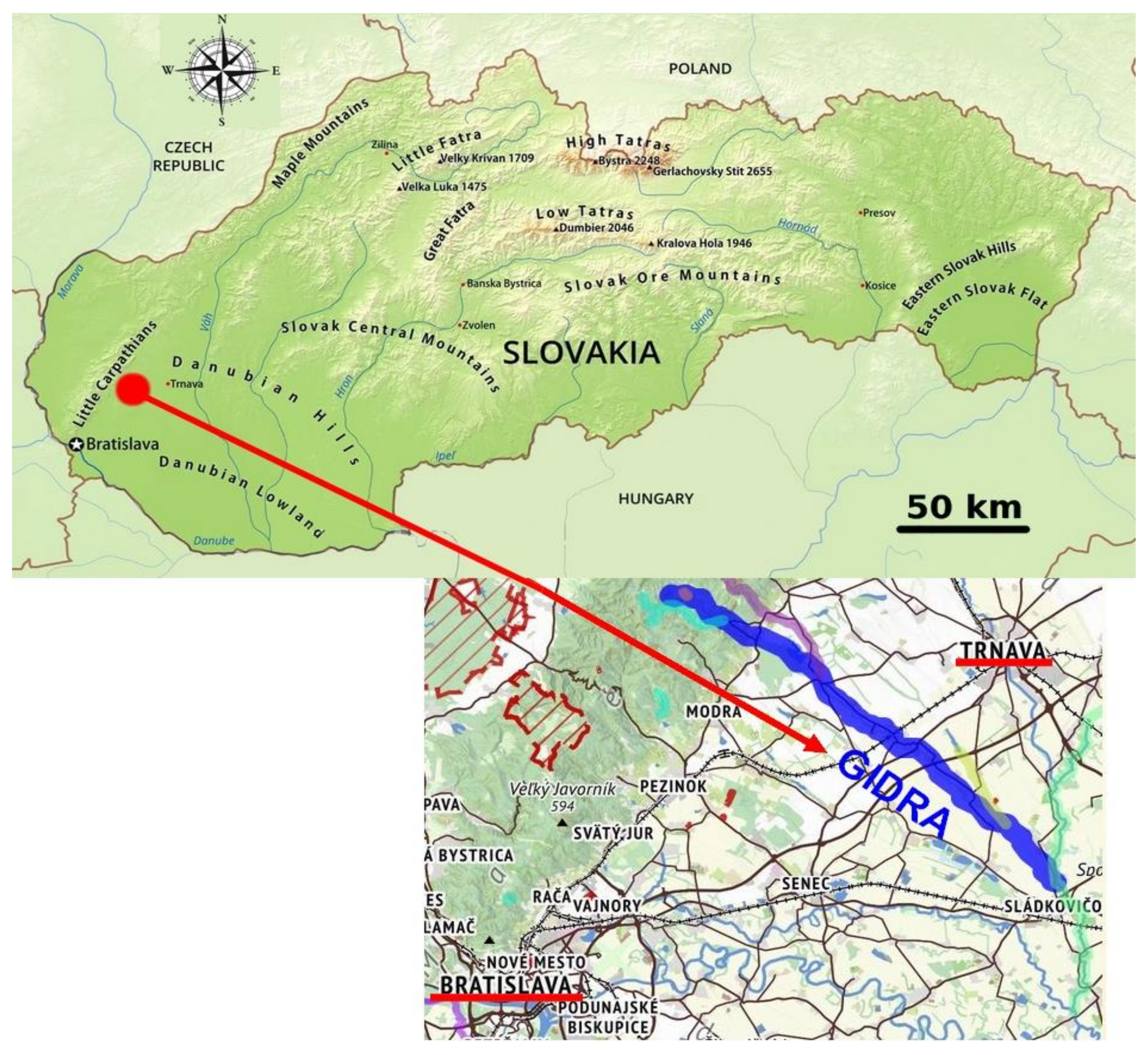
The Gidra River catchment is located above the village of Píla on the southeastern slopes of the Little Carpathians, which are situated in western Slovakia (Figure 1). The catchment is more than 95% forested [12]. These mountains belong to the southern corner of the inner Carpathian and, in their upper parts, the streams flow through the original beech forest environment.
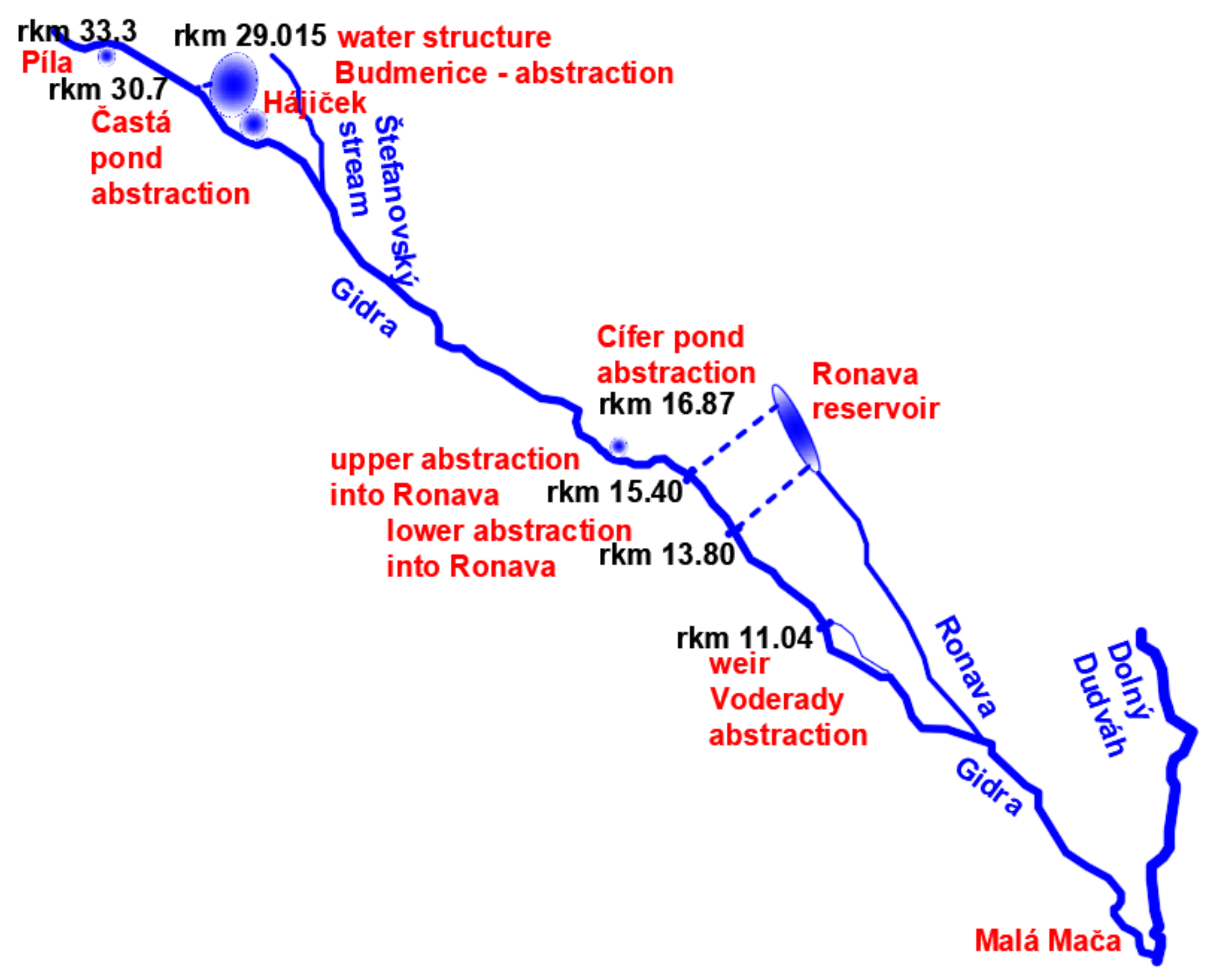
Many water abstractions exist along the Gidra River, and those water abstractions are both private and public. The drought assessment must trace every source of water whether from water abstractions, reservoirs, ponds, weirs, or fisheries to control every possibility of water loss along the river. Figure 2 shows the Gidra River and all of the existing water abstractions, which are:
- Fishery Častá [14] is a system of ponds where the water is diverted by side abstraction.
- Budmerice water structure and Hájiček pond [15] are water structures located upstream from Budmerice village, which diverts water into the Budmerice reservoir and the Gidra River.
- Pond in Cífer [16] is a throughflow pond (the volume of water flows into the pond and the other side of the pond has outflow back to the Gidra River).
- Upstream side abstraction of Voderady weir [19] is a water abstraction for supplying a small pond in the park of Voderady manor house (weir of Voderady).
Figure 2.
Gidra River and its tributaries showing all described abstractions and water structures.

The area under the mountain regions often encounters flash floods [20]. In 2018, approximately the lowest quarter of the Gidra River was completely dry according to many local observations. The reason was ambiguous and only two actions could have been taken. The first option was to trace back the volume of the water used in every abstraction along the river. Therefore, it would ensure whether there was any unusual activity or irregular water consumption that year. This method is impractical due to the missing record of water abstraction in each part of the river.
The second option was to conduct a drought assessment of the Gidra River over the past 58 years and detect all the dry periods to detach any related events. This method is set to check the effect of a continuous dry period on the groundwater level. Additionally, it allows the possibility of interpreting the situation of 2018 as a result of water infiltrating into the ground due to precedent hydrological drought events, which may have led to a decrease in the level of groundwater. Thus, the deep and machine learning models can aid in detecting any dry period in the Gidra River catchment by predicting such events in advance, thus regulating the water operations and distributions accordingly.
For the purpose of this study, the daily mean discharges over 58 years were provided by SHMI from the only gauging station, called Píla, for the period 1961–2018. The dataset contains the date of discharge in the form dd/mm/yyyy, code of gauging stations according to the SHMI, name of the stream/village, and daily mean discharges in m3·s−1.
2.2. Drought Assessment
There are various indices that are used to measure and identify drought of different types. These indices include: standardized precipitation index (SPI), standardized streamflow index (SSI), a threshold-based index, Palmer drought severity index, and snow water supply index [21]. The standardized precipitation evaporation index and the standardized snowmelt and rain index use precipitation and temperature to estimate streamflow [21].
However, most of these indices require more information than only average daily discharge to give an accurate hydrological assessment. Therefore, in such cases, the water bearing coefficient is used in Slovakia to assess the hydrological status of a given river. It compares the average discharge value of any year with the long-term average value (which represents the normal status) [13]. Exploratory data analysis is performed on daily average discharges by extracting one of basic low-flow statistics (mean flow) [22] monthly and annually, then comparing the results on monthly basis over the study period (1961–2018).
As previously mentioned, the data for the daily average discharge obtained for this study are for 58 years. The data were taken over the period 1961–2018. The hydrological situation of each year in the dataset is evaluated using the water bearing coefficient. The ratio between annual average discharge value and long-term average discharge is compared to standard values, which are defined by the normal, wet, and dry hydrological status of the river. In Table 1, the standard values of the water bearing coefficient are obtained in order to differentiate between hydrological characteristics of the river. Standard values of the water bearing coefficient represent the percentage of average discharge in a given period in comparison to the long-term average, which is demonstrated in standard intervals. The standard intervals are divided into three main categories to determine whether the year is dry, normal, or wet, and more subcategories are used to measure the severity of drought and wet years [13]. Based on those intervals, it is possible to determine the hydrological status by calculating the water bearing coefficient for each year, comparing it with the standard intervals, and then assessing the situation accordingly.
The evaluation of the hydrological situation using the water bearing coefficient for the period between 2001 and 2018 is demonstrated in Table 2. Furthermore, Table 2 consists of five columns, the first column contains the year index, while the second column has only one value (long-term average discharge Qa1961–2000 designated according to SHMI standards), the third column contains values of annual average discharge of each year in the study period, the fourth column contains the calculated water bearing coefficient for each year, and the last column contains the hydrological status of the Gidra River for each year in the study period.
2.3. Characterization of Normal and Dry Years
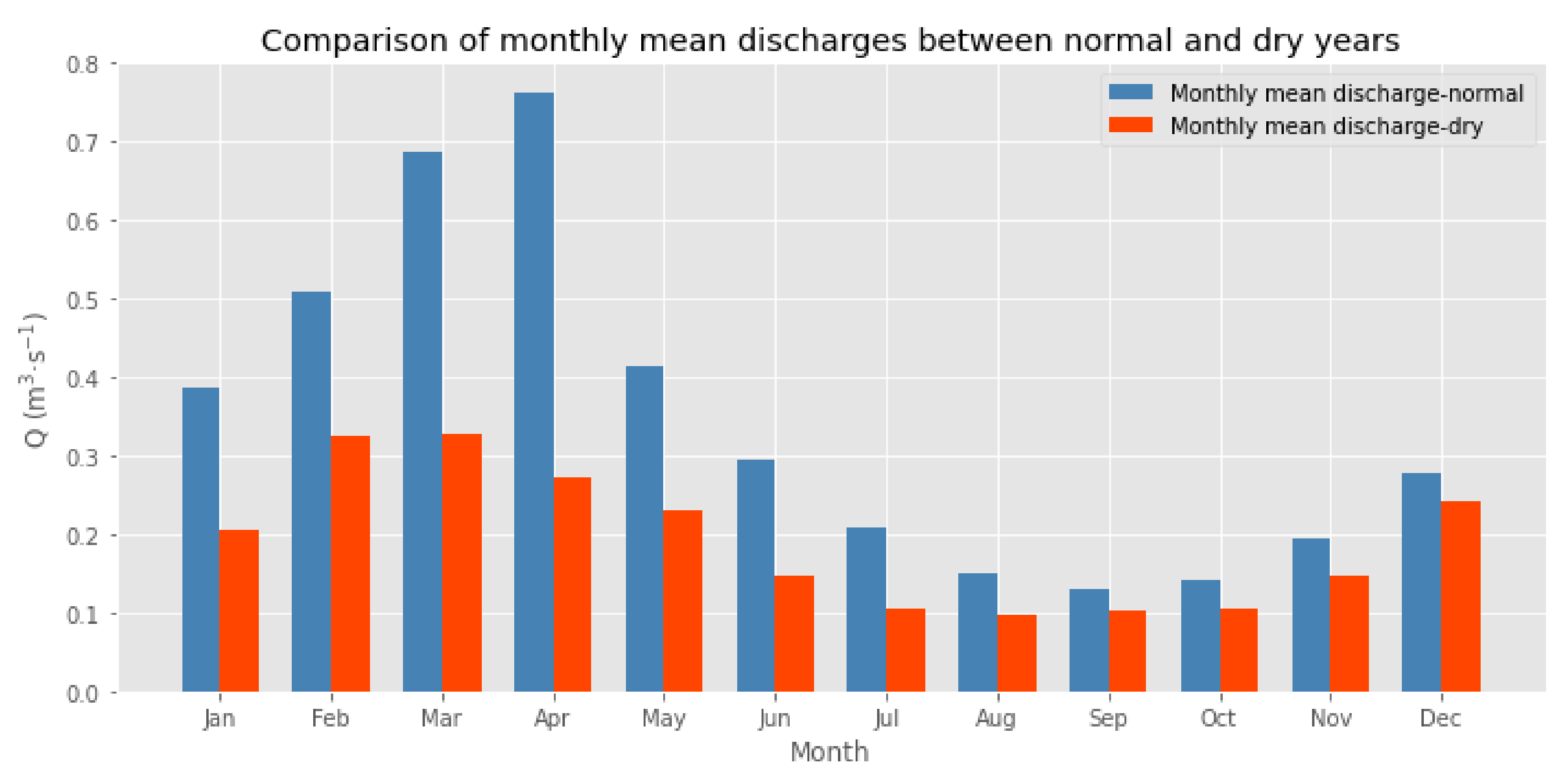
To prepare the discharge data for analyzing and modeling, the data were divided into two separate parts. The first part consists of all daily and monthly average discharges for dry years. The second part contains daily and monthly average discharges of all wet and normal assessed years, and starting from this point the notation for normal year refers to both normal and wet years. By using this methodology, it is possible to detect any existing pattern in both dry and normal parts of the data. Therefore, it is possible to extract the average monthly discharges for the long-term normal and dry hydrological years and compare them in order to find the major differences in monthly average discharges. Figure 3 illustrates the differences in monthly average discharges between normal and dry years.
Differences between monthly mean discharges in dry and normal years vary in their value each month. However, the value difference in the months of January, February, March, and April are the most significant, while the differences in mean discharges in the summer months are smaller. The monthly average discharges show a similar pattern of changes for dry and normal assessed years, as shown in Figure 3. The monthly average discharges in normal years show a steady increase in the first four months of the year, when the peak is usually reached in April. After the peak, the average monthly discharge value starts decreasing to reach the lowest value in September and then it starts to increase again until December. On the other hand, the monthly average discharges of dry years show a similar pattern with a slight difference. The values differ in the increasing/decreasing magnitude and the month of the peak/lowest average discharge over the year. A similar rising pattern was observed in the dry years, but the peak discharge value is reached in March. After the peak, the values start to decrease from March until reaching the lowest point in August, then the values follow an increasing pattern until the end of the year.
The difference in the magnitude of a sequence of monthly mean discharges between normal and dry years is most significant in the first four months. Hence, it may imply that the average discharge values of the first four months play a decisive role in determining the hydrological situation of the Gidra River for the whole year. The monthly mean discharge in April might be the most effective value to assess the hydrological situation. The monthly mean discharge in March is considered the second most effective value in this approach.
Average discharges for January, February, March, and April provided basic indicators to differentiate between the normal and dry years. For further analysis, a range comparison between the monthly average discharges for each month over the study period 1961–2018 was conducted to understand the difference between the dry and normal hydrological situation in terms of monthly average discharges.
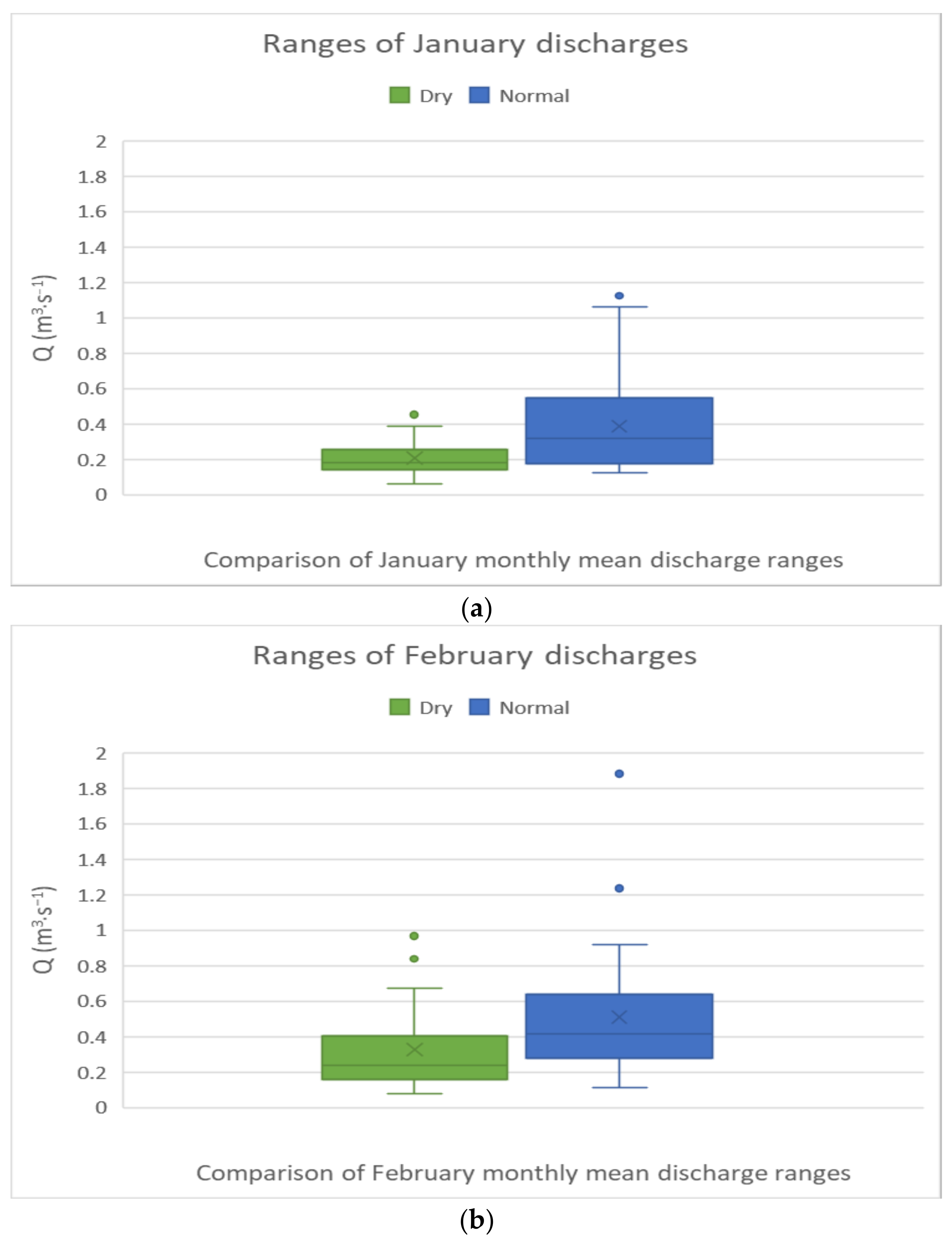
This comparison aimed to examine the overlapping rate of monthly average discharge values between normal and dry years using box plots for January, February, March, and April. Figure 4 illustrates the distribution of monthly average discharges in January and February in both dry and normal years. The boxes represent interquartile ranges (IQR), which contain 50% of the data (the discharges between 25% and 75% of the ordered data), while the horizontal line in the middle of the box represents the median. The whiskers contain the remaining data points, which their values are between (Q1 − 1.5×IQR) and (Q3 + 1.5×IQR), where Q1 is the point of 25% of the data and Q3 represents the point with the 75th percentage of the ordered data [23].
By comparing the ranges of January (Figure 4a) average discharges, a high rate of overlapping is observed. Over 50% of average discharges in normal years contain similar values as the average discharges in dry years, and over 75% of average discharges in dry years overlap with less than 50% of average discharge values in normal years. However, more than 25% of discharges in normal years did not occur in any previous dry year.
In February (Figure 4b), the situation is different, and the rate of overlapping is even higher than what is observed in January (Figure 4a). For a better understanding of monthly mean discharge distribution in normal and dry years, it is observed that 75% of average discharges in dry years overlap with 50% of average discharges in normal years, and over 50% of discharges in dry years overlap with less than 25% of discharges in normal years.
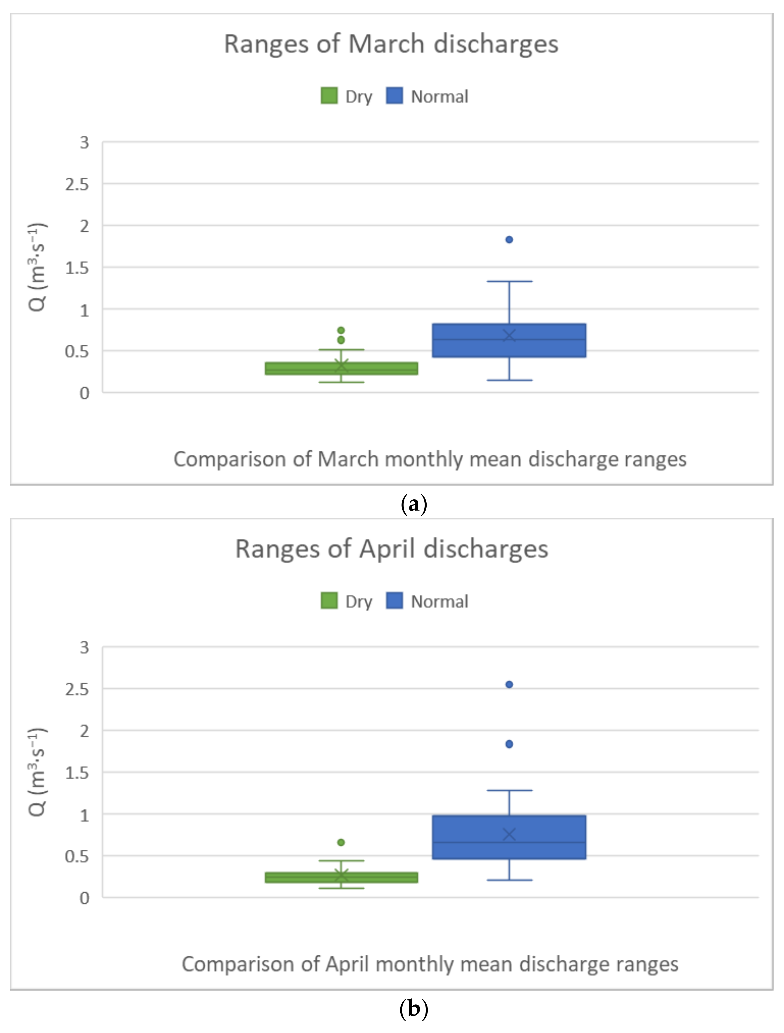
In Figure 5, the ranges of monthly mean discharges of March (Figure 5a) and April (Figure 5b) for both dry and normal years are displayed in box plots.
In March (Figure 5a), over 90% of average discharges in dry years are distributed in the range of 0–0.5 m3·s−1. Less than 30% of average discharges in normal years also fall in the same range. More than 60% of average discharges values in normal years have never occurred in any dry years, and more than 75% of average discharges in dry years are overlapping with less than 25% of discharges values in normal years. The overlapping rate in average discharges for normal and dry years is significant (around 30%, excluding outliers) over the period between 1961 and 2018. The low overlapping rate in March provides a valuable indicator to the drought assessment process.
On the other hand, the ranges of average discharge in April (Figure 5b) for both dry and normal years have a significant low overlapping rate. Over 95% of average discharges in dry years are in the range of 0–0.5 m3·s−1. Less than 30% of average discharges in normal years are in the same range. Only one extreme value of average discharges, which is classified as an outlier overlaps with 75% of average discharges in normal years.
In summary, we conclude that the variations in monthly average discharges between dry and normal years are most significant in the first four months of the year. When comparing the average discharge values for the series of months to the other series of months, the first four months had the highest difference between dry and normal situations. However, the overlapping rate of monthly average discharges for January, February, March, and April in dry and normal situations is not constant. The rate shows the probability of having similar monthly average discharge values in both dry and normal years. In order to differentiate between dry and normal hydrological situations, we have to look for the lower overlapping rate in monthly average discharges for our selected month series, as shown in Figure 4 and Figure 5. In both figures, we can see the overlapping rate in this monthly series is sorted in ascending order as follows: April, March, January, and February. Therefore, the monthly average discharge value in April is most likely to determine if a specific year is hydrologically dry or normal. However, in April the overlapping rate reaches 30%, which is highly error prone and leads to the main investigation of this paper: Based only on the discharge values of the first four months, how would it be possible to predict the situation of the Gidra River?
2.4. Modeling Process
2.4.1. Pattern Detection
Two separate patterns were extracted for dry and normal hydrological years of the Gidra River’s discharges. However, the discharges of the first four months of each year vary the most when comparing dry and normal average hydrological years. Discharge distribution for both dry and normal years has a low overlapping rate, which could be useful to differentiate between dry and normal years.
Although the difference in monthly average discharges is significant when comparing dry and normal years in the first four months, the level of overlapping in monthly average discharge distributions is complicated, especially in January and February. Hence, the modeling process is aimed to use a combination of the precedent analysis results to develop a model to classify the hydrological situation.
Thus, the modeling process is based on the following results:
- Monthly average discharge values of January, February, March, and April vary between normal and dry hydrological situations.
- The difference in monthly average discharge values of the first four months is the highest in comparison to any series of monthly discharge values.
- Monthly average discharge distribution has a low overlapping rate in March and April and a relatively moderate overlapping rate in January and February.
- The overlapping rate of monthly discharge distribution in the first four months is the lowest in comparison to any series of monthly discharges.
This pattern confirms the results of the previous study regarding hydrological droughts or periods of low flow in Slovakia [24]. The surface runoff regime in Slovakia is typically characterized by runoff increased in the spring. It occurs later in mountain areas with higher altitudes and then in lowland watercourses due to later melting of snow and larger snow reserves, both of which are important factors influencing spring runoff [24]. If the level of spring runoff decreases, the discharge rate also decreases. This trend could indicate a dry situation because the spring runoff is below natural when it is supposed to be the highest rate of the year.
2.4.2. Data Processing
Data preparation for modeling is a multistep process. This process transforms the raw data into the desired structure that is compatible with both models used in the study.
The data obtained for this study are the daily average discharge value for the period 1961–2018. The data were first used to extract monthly average discharges for drought assessment using the water bearing coefficient. Hence, the hydrological situation for each year in the dataset is determined and assigned a notation as “1” for normal and “0” for dry. The hydrological situations represent the target of the modeling process, where models should be able to classify the hydrological situation and provide the output as “1”s and “0”s for normal and dry situations, respectively.
The aim of the study is to predict the hydrological situation of the Gidra River based on the daily average discharge values of the first four months. Therefore, the inputs for the modeling process are the daily average discharge values of the first 120 days, while the desired outputs of the modeling process are the correct hydrological situation in the form of “1” for normal and “0” for dry.
The modeling process in machine learning usually includes two steps: training and testing. Thus, the data are split into two groups; the first group should contain 60–80% of the data for training, and the second group contains the other 20–40% for testing. Since the general dataset has approximately a balanced percentage of dry and normal assessed years, the normal years result in 60% over 35 years and the dry years result in 40% over 23 years. Additionally, the data over the period 1961–2000 are reserved for training, while the data over the period 2001–2018 is reserved for testing. The reason behind splitting the data in this order is to maintain the homogeneity in terms of the variety of hydrological situations and their severity for a continuous series of years.
Another reason for splitting the data in this manner is to investigate the impact of using long-term average discharge from 1961 to 2000 on the subsequent period. We used the long-term average discharge to compute the water bearing coefficient for each year, and we used the period 1961–2000 as the long-term period to measure its effect on the next period. As a result, the testing dataset over the period 2001–2018 meets the conditions for homogeneity and tests the efficacy of utilizing the long-term average value in accordance with SHMI’s recommendations.
The first group (training set) contains the daily average discharges of the first 120 days over the period 1961–2000 and the hydrological situations as the target values, while the second group (testing set) contains the daily average discharges of the first 120 days over the period 2001–2018 with the hydrological situations as the target values.
2.4.3. Model Building
The support vector machine algorithm and artificial neural network models are utilized in this study to classify the hydrological situation of the Gidra River, where the main task of both models is to predict whether the hydrological situation of the Gidra River is dry or normal, based on the data of daily average discharge of the first four months.
SVM is a popular machine learning algorithm to analyze data and recognize patterns. SVM performs classification by constructing an N-dimensional hyperplane (a plane generalized into N dimensions), which separates the data into two categories. They are used for classification and regression analysis, among other tasks [25,26].
The first step of the modeling process is splitting the data into two groups. The first group is for training the model. It contains daily average discharge values of the first four months for 40 years in the period between 1961 and 2000 as well as the hydrological situation of the Gidra River for every year over the same period. The training dataset is used to feed the model with inputs concerning daily average discharges and the resulting hydrological situation of each year; therefore, the model is able to recognize an empirical pattern (N-dimensional hyperplane) [26] and to separate the values of the daily discharge into a dry and normal situation.
Afterward, the model obtained a separable N-dimensional hyperplane, which can separate daily average discharges into two classes; dry and normal. The N-dimensional hyperplane obtained should be applicable for the testing dataset, which contains daily average discharges of the Gidra River over the validation period 2001–2018 without providing the hydrological situation of those years. The SVM model should generate results regarding the hydrological situation of the Gidra River over the testing period using the separable N-dimensional hyperplane. The outcome is generated in the format “0” for dry hydrological status and “1” for normal hydrological status.
As the real hydrological situations over the testing period 2001–2018 are evaluated in this study, it is possible to measure the accuracy of the model’s results (predicted-status) by comparing them with the real hydrological situations over the testing period (real-status). Table 3 shows the predicted results of the hydrological situation over the testing period 2001–2018, which are identical to the real assessed values.
The second model developed in this study is based on the deep neural network model. It provides similar results while employing a more complex technique. Although the definition of the neural network is not the object of this study, for a better understanding of the concept a brief definition is necessary. The neural network is a parametric supervised deep learning algorithm that contains N layers. It takes inputs as an N-dimensional array then it applies nonlinear transformation (by using multiple activation functions) on the input values by multiplying them by learnable parameters and constantly tuning those parameters until the output of this model satisfies the required outputs in the learning phase [25,27]. This process is called backpropagation and it requires three steps: loss functions to measure the difference between predicted outputs and the real outputs, metric function to measure the accuracy of the model, and an optimization algorithm to estimate the parameter values depending on the values of the loss function.
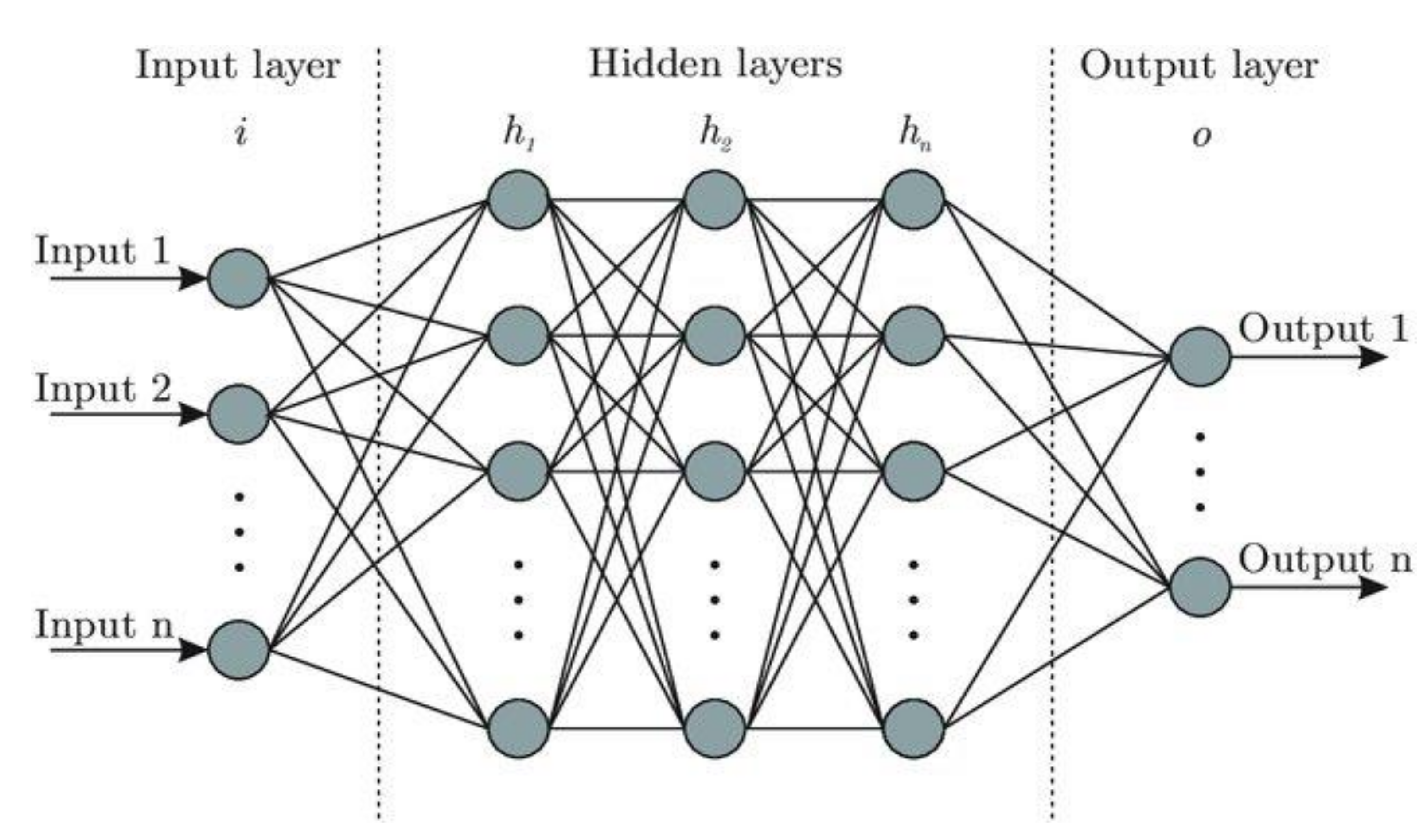
The inputs of this model are the daily average discharges of the first 120 days of each year in the training dataset. Therefore, the input layer of this model should contain 120 neurons. Equation (1) refers to the computations that are performed across every neuron in the network. In each neuron “k” of any hidden layers, a nonlinear transformation is applied to the weighted sum (with weights wk,1, …, wk,n) of its linear input n (which are inherited from previous layers, as shown in Figure 6) plus a bias b, whereas w, b are the accumulated parameters. The output yk is constantly passed to the next layer after transforming the inputs nonlinearly using activation functions g.
The neural network model used to classify the hydrological situation of the Gidra River contains six layers (including the input layer); each layer has a defined number of neurons (120, 90, 60, 30, 4, 1), respectively. It is used in the following nonlinear activation functions: scaled exponential linear unit (SELU, Equation (2), where α, λ are justified according to [29]), hyperbolic tangent (tanh, Equation (3)), and Softplus, Equation (4) [30]. For parameter optimization, a cosine similarity function is used as a loss function and the binary cross-entropy function is used as a metric function [30]. The stochastic gradient descent algorithm is used as an optimization algorithm to tune the parameters with a learning rate set to 0.1.
Additionally, one specific step has been used before feeding training data to the ANN model, and that is scaling input data using a robust scaler to transform the input values into values that are robust to outliers. Equation (5) shows the mathematical representation of a robust scaler that removes the median and scales the data in the range between 1st quartile and 3rd quartile by subtracting the median (xmid) and then dividing by the interquartile range (75% value–25% value), i.e., in between the 25th quartile and 75th quartile range (x75 − x25). If outliers are present in the dataset, then the median and the interquartile range provide better results and outperform the sample mean and variance [30].
3. Results and Discussion
3.1. Modeling Results
The SVM and ANN models have been trained on the training dataset to obtain the required parameters for accurate predictions of the hydrological situation of the Gidra River. The SVM model has 120 parameters, whereas the ANN model has 120, 90, 60, 30, and 4 parameters based on the number of neurons in each layer. The parameters of both models have been calibrated using the mathematical theory of support vector machines and backpropagation [25,26,27]. Both models show accurate results predicting the hydrological situation of the training dataset. The input of the testing dataset was introduced to both models and the predicted hydrological situations (output) were compared with the real hydrological situations for the period 2001–2018. Table 3 compares predicted and real status over the testing period for both models, where the second column represents the real hydrological status, and the third column represents the predicted values of hydrological status. As shown in Table 3, the real and predicted hydrological status are identical, which indicates that the SVM model with a linear kernel and ANN were successful in predicting the drought situation of the Gidra River correctly during the period 2001–2018.
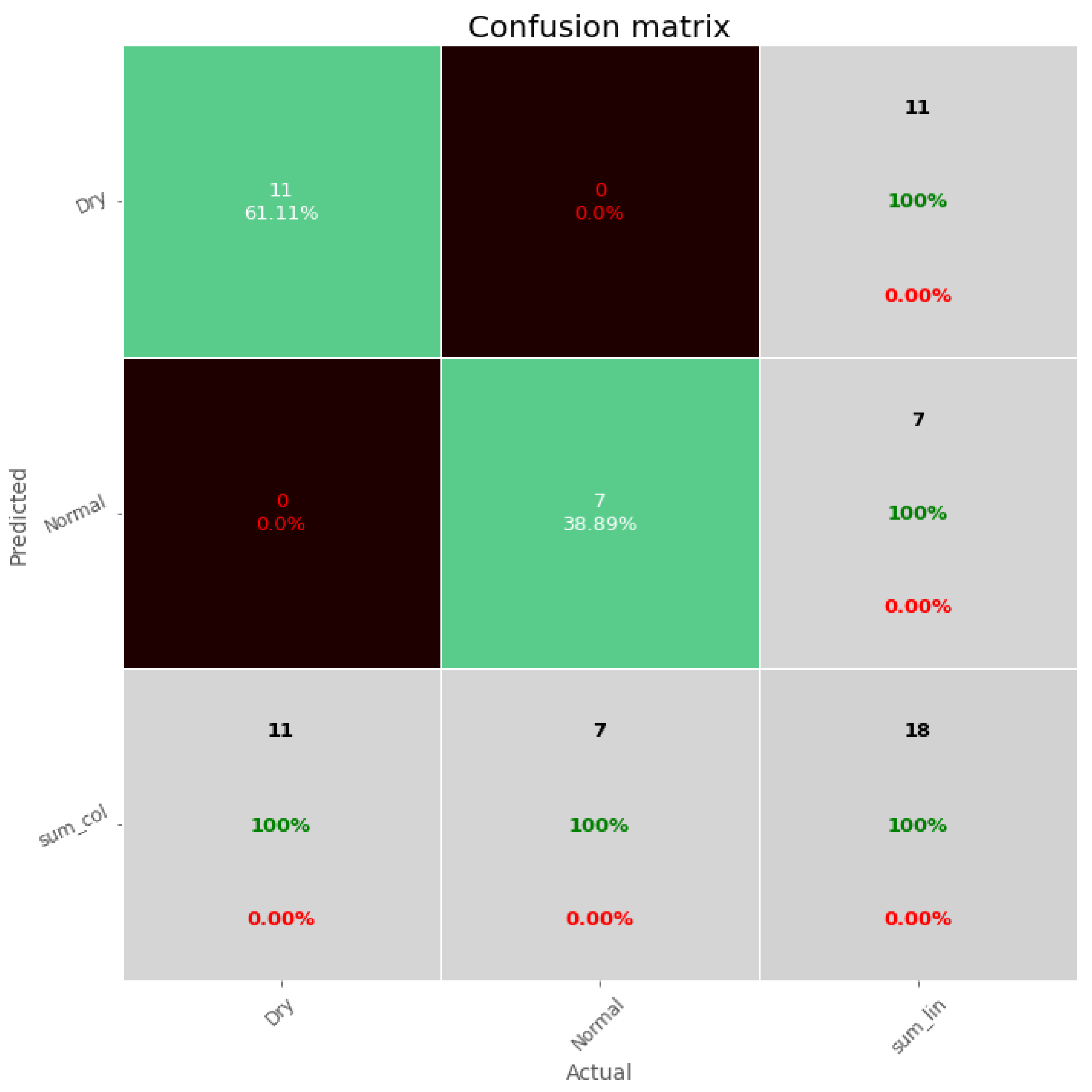
A confusion matrix is used to visualize the accuracy of both models, as shown in Figure 7. Both models succeeded in predicting the drought hydrological situation in the Gidra River on the testing dataset. It correctly classified 11 years as dry years using only daily average discharges of the first four months of each year, as shown in Figure 7.
For verifying the accuracy of both models, the data of years 2019 and 2020 were provided, but only the daily discharges of the first four months of both years. This was used to test the forecasting model results and compare them with the assessment of SHMI for the hydrological situation on the Gidra River. Both SVM and ANN models show results of the dry hydrological situation for 2019 and 2020, which correspond with the results obtained from the analysis using SHMI methodology (water bearing coefficient values for 2019 and 2020: 72 and 85, respectively) and drought assessment by SHMI [31,32].
3.2. Comparison with Previous Studies
This study examined the performance of two well-known machine learning models, SVM and ANN, in predicting the hydrological drought of the Gidra River. Many researchers have been testing the efficiency of deploying both models to predict drought situations in different parts of the world. Furthermore, a recent study was conducted in Pakistan to predict drought in various locations using SVM and ANN [33]. SVM proved to be more efficient in capturing characteristics of drought development and severity over Pakistan. Moreover, SVM outperformed ANN in predicting extreme drought situations in a certain season [33]. In this study, both models provided the exact same results over the testing period. However, the input data and model complexity play a major role in determining the output precision and the input data of this research was restricted to only daily average discharge values.
Another study utilized ANN and SVM to evaluate and predict drought situations in multiple rivers in the United States of America [34]. The study showed that the performance of the models correlates with the location, type, and snowmelt process in the mountains. Both models reached their best performance for predicting drought in the Chehalis River while the poorest performance appeared in the Carson River drought prediction, owing to the time difference between streamflow and snowmelt in these two river basins [34]. These results confirm that the performance of any model may change for different locations and it highly depends on snowmelt parameters [34]
3.3. Discussion
This study showed high accuracy of SVM and ANN results in classifying the hydrological drought. The inputs for both models were the values of daily average discharges of the first 120 days. After training, the SVM model showed perfect performance in classifying the hydrological situations linearly in a high dimensional space of 120 features (inputs). The possibility of linearly separating the data inputs into two classes indicates a low level of data complexity. However, this result does not apply to all possible training sets in case the data were split differently. Thus, this confirms the effect of splitting the data homogeneously, meaning that the training dataset should contain a variety of hydrological situations with different water bearing coefficient values, especially for values located around the limits of determining a new hydrological situation; more specifically, when the input data are of one type, the daily average discharge values, as in this case.
As previously mentioned, ANN is a more complex parametric model that requires more information to set up. It requires the loss function, the optimizer, the activation functions for each layer, the number of neurons in each layer, the overall architecture of the network, and input data transformation. Multiple data transformations such as normalization, standardization, and scaling may apply to the raw data before using the data for training and testing purposes. These transformations tend to boost the model accuracy.
Vanishing gradient descent is one of the frequent problems that appear when using sigmoid activation functions in the deep ANN model. Instead, it is possible to use tanh and SELU activation functions after scaling the data to overcome this problem. Moreover, random initialization of the parameters w, b for the ANN model is one way of avoiding vanishing gradient descent in the training phase; however, use of the Xavier parameters initializing method is recommended to enhance accuracy in the validation phase by choosing model parameters in a systematic approach [35].
Reaching 100% accuracy in ANN models is a surprising result and, it was at first considered a result of overfitting. However, the same results were reached in the SVM model applying linear kernel to classify the hydrological situation in the Gidra River. Therefore, the ability to reach the same results using a linear kernel in the SVM model negates the overfitting effect on the ANN model. After performing multiple experiences with the different training sets, the ANN model obtained better results and, in many cases, these results seem to contain information about the drought severity.
The drawback of both models is their dependency on a single type of data as input. For example, both models do not take into consideration other types of hydrological data, such as temperature, water ground level, and snowmelt, which may expedite the development of drought periods.
These findings apply to foothill rivers, as well. It is more likely that the behavior of rivers in the lowlands could have different patterns. It depends on the flow regime in channels or surface water at lowland territories during the growing season. This often is strongly influenced by the occurrence of aquatic vegetation [36]. As a result, implementing such models to different climate regimes should involve considering other factors that may be more related to droughts in the target climatic area.
4. Conclusions
Analyzing historical data of different types (hydrological, meteorological, climatological, and many others) for drought assessment is one of many possible ways to characterize drought and dry periods. However, performing a broad statistical analysis on hydrological data for any river or streamflow reveals valuable information about average discharges, ranges of average discharges, and the typical average year of dry and normal hydrological situations.
For the Gidra River, after performing detailed statistical analysis according to the SHMI methods, the following results were obtained:
- The discharges of January, February, March, and April play a major role in the final hydrological situation of the Gidra River.
- There is a significant difference in average discharge values for the first four months between dry and normal assessed years.
- Drought has a significant impact on monthly average discharges, mainly in March and April, because it is a stream below a mountainous region and influenced by snowmelt.
- It is possible to use historical data and deploy machine learning models to predict the hydrological situation.
- More accurate results on the hydrological situation obtained from precipitation and snowcover data are recommended to consider, analyze, and combine with discharge values to track every possible pattern through time.
The results of the study provide useful information for any operation project of the Gidra River, including water distribution for agriculture or any other purposes, owing to the number of water structures and abstractions along the river. To prevent downstream drying, forecasting the hydrological status of the Gidra River based on daily discharges during the first four months of the year could be included in the operating manuals for water structures on the Gidra River.
Author Contributions
Conceptualization, L.Č. and W.A.; methodology, L.Č. and W.A.; software, W.A.; validation, W.A.; formal analysis, L.Č., W.A. and A.Š.; investigation, L.Č. and W.A.; resources, L.Č. and W.A.; data curation, L.Č. and W.A.; writing—original draft preparation, L.Č., W.A. and A.Š.; writing—review and editing, L.Č., W.A. and A.Š.; visualization, L.Č. and W.A.; supervision, A.Š.; project administration, A.Š. All authors have read and agreed to the published version of the manuscript.
Funding
This research received no external funding.
Institutional Review Board Statement
Not applicable.
Informed Consent Statement
Not applicable.
Acknowledgments
This contribution was developed within the framework and based on the financial support of the APVV-19-0383 project, “Natural and technical measures oriented to water retention in sub-mountain watersheds of Slovakia”, together with VEGA project No. 1/0728/21, “Analysis and prognosis of the impact of construction activities on groundwater in urbanized territory”.
Conflicts of Interest
The authors declare no conflict of interest.
References
- Lloyd-Hughes, B. The impracticality of a universal drought definition. Theor. Appl. Climatol. 2013, 117, 607–611. [Google Scholar] [CrossRef] [Green Version]
- Kandra, B.; Gomboš, M. Influence of climatic elements on the water regime in a soil profile. Cereal Res. Commun. 2008, 36 (Suppl. 5), 1187–1190. [Google Scholar]
- European Environment Agency. Climate Change and Water Adaptation Issues; European Environment Agency: Copenhagen, Denmark, 2007; p. 112. [Google Scholar]
- Wood, E.; Sheffield, J. The Science of Drought. In Drought: Past Problems and Future Scenarios; Taylor and Francis: Abingdon, UK, 2012; pp. 3–26. [Google Scholar]
- Yevjevich, V. An objective approach to definitions and investigations of continental hydrologic droughts. J. Hydrol. 1969, 7, 353. [Google Scholar]
- Alsumaiei, A.; Alrashidi, M. Hydrometeorological Drought Forecasting in Hyper-Arid Climates Using Nonlinear Autoregressive Neural Networks. Water 2020, 12, 2611. [Google Scholar] [CrossRef]
- Mosavi, A.; Ozturk, P.; Chau, K. Flood Prediction Using Machine Learning Models: Literature Review. Water 2018, 10, 1536. [Google Scholar] [CrossRef] [Green Version]
- Mishra, A.; Desai, V. Drought forecasting using stochastic models. Stoch. Environ. Res. Risk Assess. 2005, 19, 326–339. [Google Scholar] [CrossRef]
- Alsumaiei, A. Monitoring Hydrometeorological Droughts Using a Simplified Precipitation Index. Climate 2020, 8, 19. [Google Scholar] [CrossRef] [Green Version]
- Belayneh, A.; Adamowski, J.; Khalil, B.; Ozga-Zielinski, B. Long-term SPI drought forecasting in the Awash River Basin in Ethiopia using wavelet neural network and wavelet support vector regression models. J. Hydrol. 2014, 508, 418–429. [Google Scholar] [CrossRef]
- Global Water Partnership Central and Eastern Europe. Guidelines for the Preparation of Drought Management Plans. Development and Implementation in the Context of the EU Water Framework Directive; Global Water Partnership Central and Eastern Europe: Stockholm, Sweden, 2015; p. 48. [Google Scholar]
- Orfánus, T.; Jenčo, M.; Bebej, J.; Benko, M. Simulation of the effects of forest roads on stormflow generation using GIS and 2D vadose zone hydrological model. Ekológia 2017, 36, 25–39. [Google Scholar] [CrossRef] [Green Version]
- Voda.oma.sk. n.d. Gidra. Available online: https://voda.oma.sk/gidra (accessed on 17 September 2021).
- Simanová, I. Operational Manual for Water Structure “Častá–Completion of Ponds” on the Gidra River at km 30.7; Proma Ltd.: Bratislava, Slovakia, 2019; p. 97. [Google Scholar]
- Magula, P. Operational Manual for Water Structure Budmerice on the Gidra River at km 29.015 (Abstraction); Slovak Water Management Company: Piešťany, Slovakia, 2012; p. 49. [Google Scholar]
- Magula, P. Operational Manual for Permanent Operation of Hájiček Pond in Budmerice (Side Reservoir on the Gidra River); Geohydro: Bratislava, Slovakia, 2007; p. 28. [Google Scholar]
- Ďuriš, V. Technical report. Measurement after the Implementation of the Sluice Weir for the Pond in Cífer and the Supply Channel to the pond; CS, Ltd.: Trnava, Slovakia, 2019; p. 7. [Google Scholar]
- Matulík, Š. Operational Manual for Water Structure Water Reservoir Ronava, Update 2019; AGROPROJEKT Nitra Ltd.: Nitra, Bratislava, Slovakia, 2019; p. 36. [Google Scholar]
- Potisk, F. Operational Manual for Water Structure Weir on the Gidra River in the River Kilometre 10.967; Slovak Water Management Company: Bratislava, Slovakia, 2018; p. 36. [Google Scholar]
- Duchan, D.; Dráb, A.; Říha, J. Flood Protection in the Czech Republic. In Management of Water Quality and Quantity; Springer: Cham, Switzerland, 2019; pp. 333–363. [Google Scholar]
- Svoboda, M.; Fuchs, B.A. Handbook of Drought Indicators and Indices Integrated Drought Management Programme (IDMP); World Meteorological Organization (WMO) and Global Water Partnership (GWP): Geneva, Switzerland, 2016; 55p. [Google Scholar]
- World Meteorological Organization. Manual on Low-Flow Estimation and Prediction; World Meteorological Organization: Geneva, Switzerland, 2008; 138p. [Google Scholar]
- McGill, R.; Tukey, J.W.; Larsen, W.A. Variations of box plots. Am. Stat. 1978, 32, 12–16. [Google Scholar]
- Bochníček, O.; Blaškovičová, L.; Damborská, I.; Fendek, M.; Fendeková, M.; Horvát, O.; Pekárová, P.; Slivová, V.; Vrablíková, D. Hydrological Drought and Its Manifestation. In Surface Water Flows, Prognosis of Hydrological Drought Development in Slovakia; Fendeková, M., Blaškovičová, L., Eds.; Comenius University: Bratislava, Slovakia, 2018; 21p. [Google Scholar]
- Farber, R. CUDA for Real Problems. In CUDA Application Design and Development; Farber, R., Ed.; Morgan Kaufmann Publishers: Burlington, MA, USA, 2011; pp. 265–275. [Google Scholar]
- Smola, A.J.; Schölkopf, B. A tutorial on support vector regression. Stat. Comput. 2004, 14, 199–222. [Google Scholar] [CrossRef] [Green Version]
- McCulloch, W.S.; Pitts, W. A logical calculus of the ideas immanent in nervous activity. Bull. Math. Biophys. 1943, 5, 115–133. [Google Scholar] [CrossRef]
- Bre, F.; Gimenez, J.M.; Fachinotti, V.D. Prediction of wind pressure coefficients on building surfaces using artificial neural networks. Energy Build. 2017, 158, 1429–1441. [Google Scholar] [CrossRef]
- Klambauer, G.; Unterthiner, T.; Mayr, A.; Hochreiter, S. Self-Normalizing Neural Networks. 2017. Available online: https://arxiv.org/abs/1706.02515. (accessed on 30 November 2021).
- Pedregosa, F.; Varoquaux, G.; Gramfort, A.; Michel, V.; Thirion, B.; Grisel, O.; Blondel, M.; Prettenhofer, P.; Weiss, R.; Dubourg, V.; et al. Scikit-learn: Machine Learning in Python. J. Mach. Learn. Res. 2011, 12, 2825–2830. [Google Scholar]
- Jeneiová, K.; Janečková, L.; Blaškovičová, L.; Podolinska, J.; Síčová, B.; Liová, S. Zhodnotenie hydrologického roka 2019 (in Slovak). Vodohospodársky Sprav. 2020, 3–4, 20–24. [Google Scholar]
- Jeneiová, K.; Blaškovičová, L.; Podolinska, J.; Slivková, K.; Síčová, B.; Liová, S. Zhodnotenie hydrologického roka 2020 (in Slovak). Vodohospodársky Sprav. 2021, 3–4, 20–24. [Google Scholar]
- Khan, N.; Sachindra, D.A.; Shahid, S.; Ahmed, K.; Shiru, M.S.; Nawaz, N. Prediction of droughts over Pakistan using machine learning algorithms. Adv. Water Resour. 2020, 139, 103562. [Google Scholar] [CrossRef]
- Parisouj, P.; Mohebzadeh, H.; Lee, T. Employing machine learning algorithms for streamflow prediction: A case study of four river basins with different climatic zones in the United States. Water Resour. Manag. 2020, 34, 4113–4131. [Google Scholar] [CrossRef]
- Glorot, X.; Bengio, Y. Understanding the difficulty of training deep feedforward neural networks. In Proceedings of the Thirteenth International Conference on Artificial Intelligence and Statistics, Sardinia, Italy, 13–15 May 2010. [Google Scholar]
- Velísková, Y.; Dulovičová, R.; Schügerl, R. Impact of vegetation on flow in a lowland stream during the growing season. Biologia 2017, 72, 840–846. [Google Scholar] [CrossRef]
Figure 1.
Location of the research area (Gidra River basin) in Slovakia [13].
Figure 1.
Location of the research area (Gidra River basin) in Slovakia [13].

Figure 3.
Monthly mean discharges for dry and normal years for the period 1961–2018.

Figure 4.
Range comparison in January (a) and February (b) for the monthly mean discharges.

Figure 5.
Range comparison in March (a) and April (b) for the monthly mean discharges.

Figure 6.
Artificial neural network architecture sketch for illustration [28].
Figure 6.
Artificial neural network architecture sketch for illustration [28].

Figure 7.
Confusion matrix for testing the classification accuracy of the SVM and ANN models.


Table 1.
Standard values of water bearing coefficient [6].
Table 1.
Standard values of water bearing coefficient [6].
| Hydrological Situation | Water Bearing Coefficient Values (%) |
|---|---|
| DRY | 10–29 |
| 30–49 | |
| 50–69 | |
| 70–89 | |
| NORMAL | 90–110 |
| WET | 111–130 |
| 131–150 | |
| 151–170 | |
| 171–180 | |
| More |
Table 2.
Assessment of hydrological status of the Gidra River using water bearing coefficient values.
Table 2.
Assessment of hydrological status of the Gidra River using water bearing coefficient values.
| Year | Qa1961–2000 (m3·s−1) | Qavg (m3·s−1) | Water Bearing Coefficient Qavg/Qa (%) | Status |
|---|---|---|---|---|
| 2001 | 0.297 | 0.181 | 60.8 | Dry |
| 2002 | 0.297 | 0.258 | 86.8 | Dry |
| 2003 | 0.297 | 0.172 | 57.8 | Dry |
| 2004 | 0.297 | 0.265 | 89.1 | Normal or wet |
| 2005 | 0.297 | 0.195 | 65.8 | Dry |
| 2006 | 0.297 | 0.462 | 155.5 | Normal or wet |
| 2007 | 0.297 | 0.187 | 63.0 | Dry |
| 2008 | 0.297 | 0.110 | 36.9 | Dry |
| 2009 | 0.297 | 0.372 | 125.4 | Normal or wet |
| 2010 | 0.297 | 0.553 | 186.3 | Normal or wet |
| 2011 | 0.297 | 0.379 | 127.5 | Normal or wet |
| 2012 | 0.297 | 0.151 | 50.7 | Dry |
| 2013 | 0.297 | 0.348 | 117.2 | Normal or wet |
| 2014 | 0.297 | 0.239 | 80.6 | Dry |
| 2015 | 0.297 | 0.304 | 102.2 | Normal or wet |
| 2016 | 0.297 | 0.220 | 74.2 | Dry |
| 2017 | 0.297 | 0.105 | 35.4 | Dry |
| 2018 | 0.297 | 0.149 | 50.2 | Dry |
Table 3.
Predicted and real hydrological status comparison over the testing period 2001–2018 using SVM and ANNs models.
Table 3.
Predicted and real hydrological status comparison over the testing period 2001–2018 using SVM and ANNs models.
| Year | Real Situation | Predicted Situation |
|---|---|---|
| 2001 | 0 | 0 |
| 2002 | 0 | 0 |
| 2003 | 0 | 0 |
| 2004 | 1 | 1 |
| 2005 | 0 | 0 |
| 2006 | 1 | 1 |
| 2007 | 0 | 0 |
| 2008 | 0 | 0 |
| 2009 | 1 | 1 |
| 2010 | 1 | 1 |
| 2011 | 1 | 1 |
| 2012 | 0 | 0 |
| 2013 | 1 | 1 |
| 2014 | 0 | 0 |
| 2015 | 1 | 1 |
| 2016 | 0 | 0 |
| 2017 | 0 | 0 |
| 2018 | 0 | 0 |
Publisher’s Note: MDPI stays neutral with regard to jurisdictional claims in published maps and institutional affiliations. |
© 2022 by the authors. Licensee MDPI, Basel, Switzerland. This article is an open access article distributed under the terms and conditions of the Creative Commons Attribution (CC BY) license (https://creativecommons.org/licenses/by/4.0/).
Share and Cite
MDPI and ACS Style
Almikaeel, W.; Čubanová, L.; Šoltész, A. Hydrological Drought Forecasting Using Machine Learning—Gidra River Case Study. Water 2022, 14, 387. https://doi.org/10.3390/w14030387
AMA Style
Almikaeel W, Čubanová L, Šoltész A. Hydrological Drought Forecasting Using Machine Learning—Gidra River Case Study. Water. 2022; 14(3):387. https://doi.org/10.3390/w14030387
Chicago/Turabian StyleAlmikaeel, Wael, Lea Čubanová, and Andrej Šoltész. 2022. "Hydrological Drought Forecasting Using Machine Learning—Gidra River Case Study" Water 14, no. 3: 387. https://doi.org/10.3390/w14030387
Note that from the first issue of 2016, this journal uses article numbers instead of page numbers. See further details here.