Rainstorm Magnitude and Debris Flows in Pyroclastic Deposits Covering Steep Slopes of Karst Reliefs in San Martino Valle Caudina (Campania, Southern Italy)

Abstract

Debris flows that have occurred in the area of San Martino Valle Caudina (Campania, Southern Italy) are described by geomorphological and hydrological analyses, focusing on the recent event of December 2019. This area can be considered a key example for studying debris-flow phenomena involving the pyroclastic mantle that covers the karstified bedrock along steep slopes. A hydrological analysis of the time series of the maximum annual rainfall, of durations of 1, 3, 6, 12 and 24 h, was carried out based on a new approach to assess rainstorm magnitude. It was quantified by measuring the deviation of the rainfall intensity from the normal conditions, within a specified time period. As the time series of annual maxima are typically skewed, a preliminary transformation is needed to normalize the distribution; to obtain the Z-value of the standard normal distribution, with mean µ = 0 and standard deviation σ = 1, different probability distribution functions were fitted to the actual data. A specific boxplot was used, with box width Z = ±1 and whiskers length Z = ±2. The deviations from these values provide the performance of the distribution fits. For the normalized time series, the rates shown by the trends and relative significance were investigated for the available time series of 11 rain gauges covering the Western–Central Campania region. The most critical condition for the debris-flow initiation appears to occur when a severe or extreme rainfall has a duration ≥ 12 h. The trend analysis did not detect statistically significant increases in the intensity of the rainfall of duration ≥ 6 h.

1. Introduction

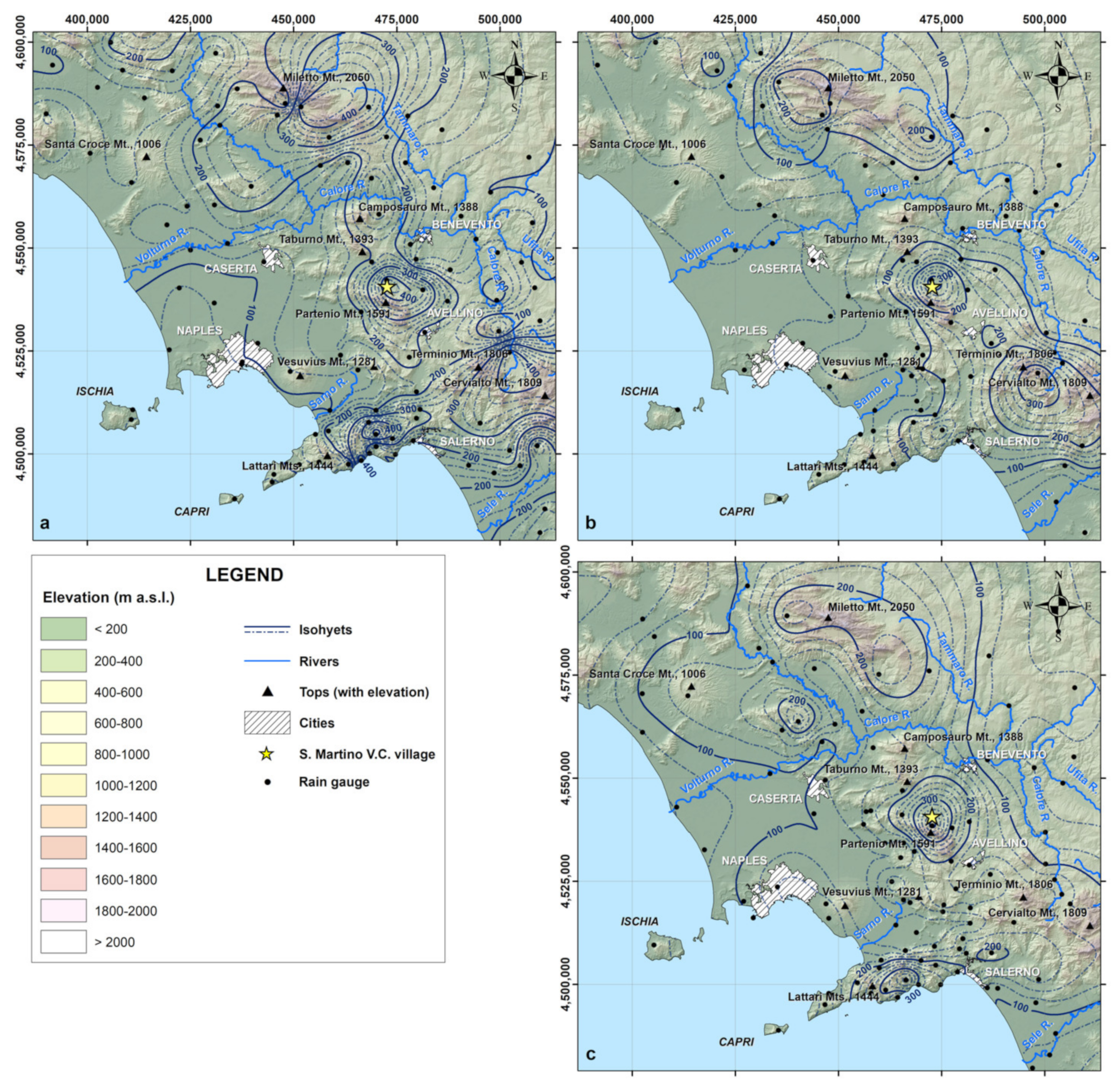
In recent years, great attention has been dedicated to the study of changes in the frequency of intense rainstorms and the increase in the severity of rainfall events. The interest in these topics has increased, especially for those areas where rainfall represents the main driver of catastrophic events, such as floods and debris flows. In Southern Italy, and particularly in the areas surrounding the Somma-Vesuvius and Phlegraean Fields, rainfall-induced debris flows are one of the main sources of risk for urban settlements. In fact, these areas have been affected by catastrophic debris flows many times in the past, characterized by rapid mobilization of the pyroclastic deposits covering the karstified calcareous bedrock [1,2,3]. Although the mechanisms that predispose these areas to slope failure are still debated in many cases cf. [4,5,6,7,8,9], the triggering of these debris flows has often been related to the occurrence of intense rainstorms. As in other areas of the world, the amount of the antecedent rainfall also has an important influence on landslides’ initiation [10]. In fact, these debris flows can occur both during extraordinary storms and less powerful storms in Campania. The extraordinary storm of 26 October 1954 that occurred along the Amalfi Coast (Lattari Mts. 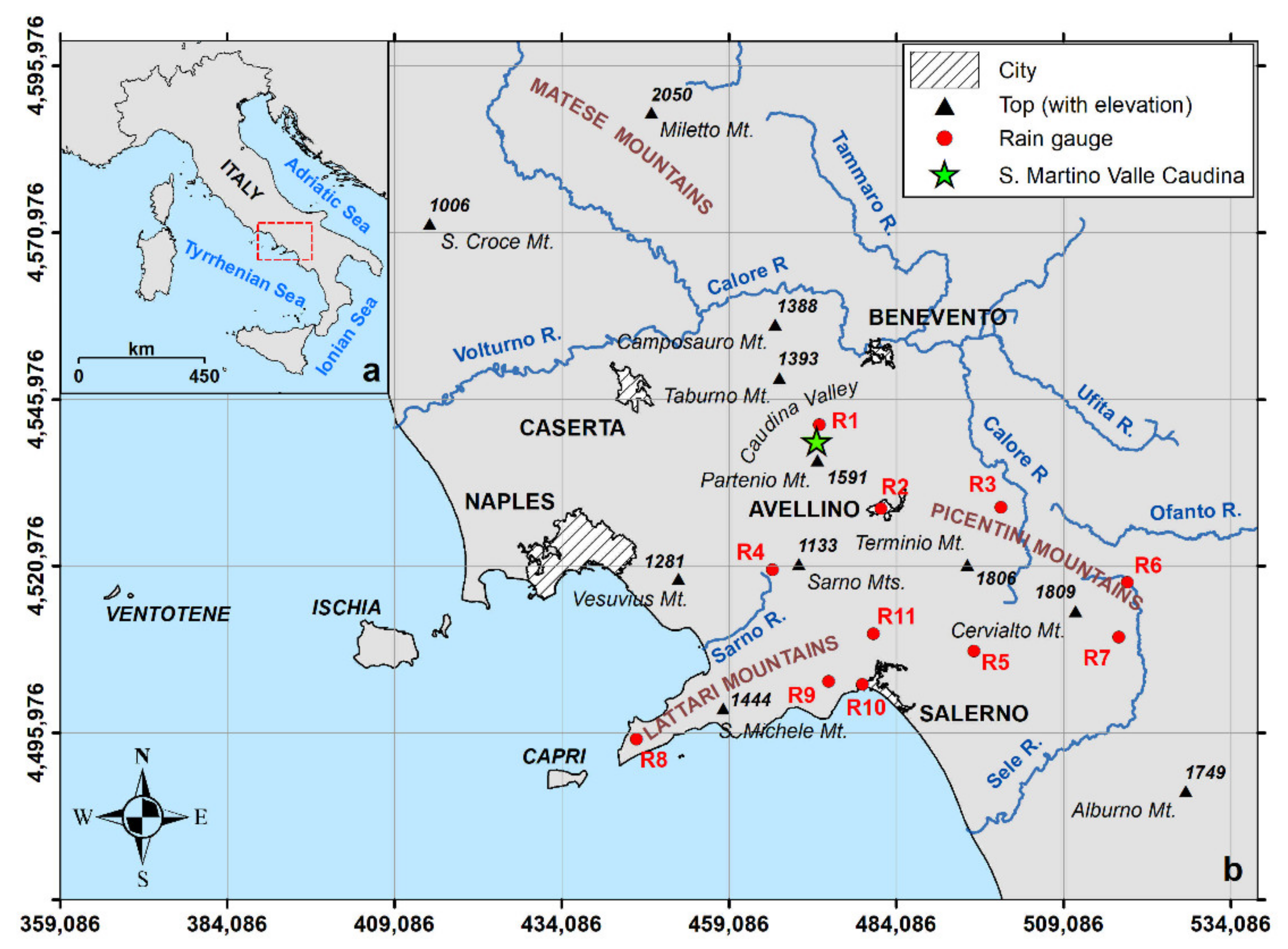in Figure 1), falls into the first category, with 459 mm in 6 h [11] and after a long dry period [4]. It caused more than 300 deaths and severe damage to infrastructures, buildings and local agriculture. The landslides that occurred in May 1998 on the Sarno Mts. (Figure 1) can be considered an example of the second category. These debris flows hit many villages (e.g., see References [2,12]) causing 130 deaths, and were induced by a prolonged storm (154.8 mm in 31 h [11]), after a very wet period [4,13].

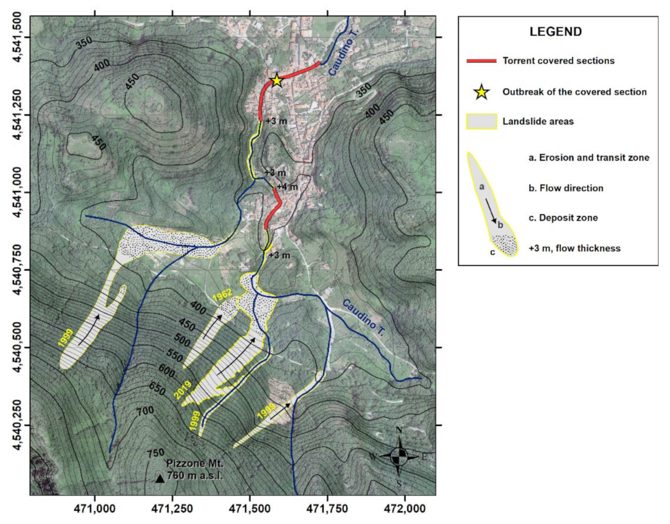
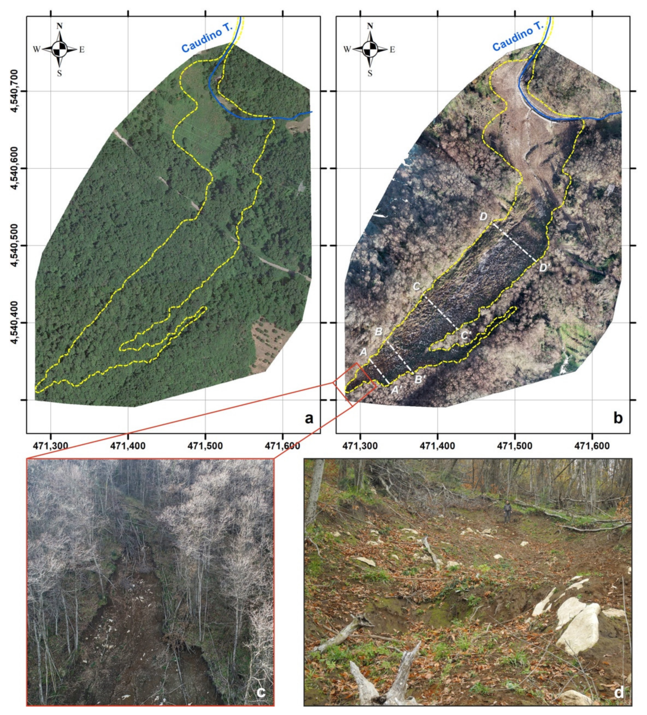
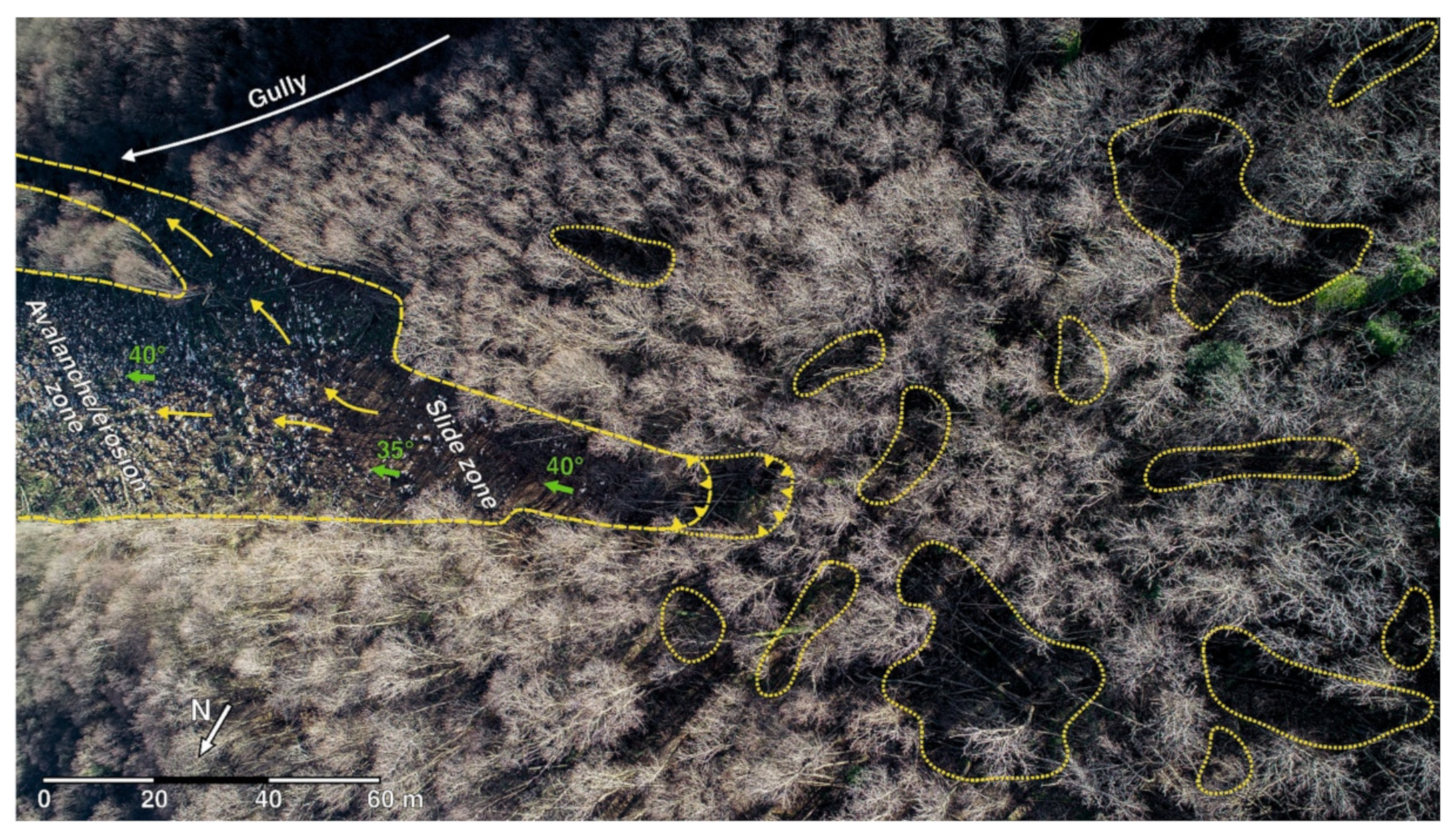
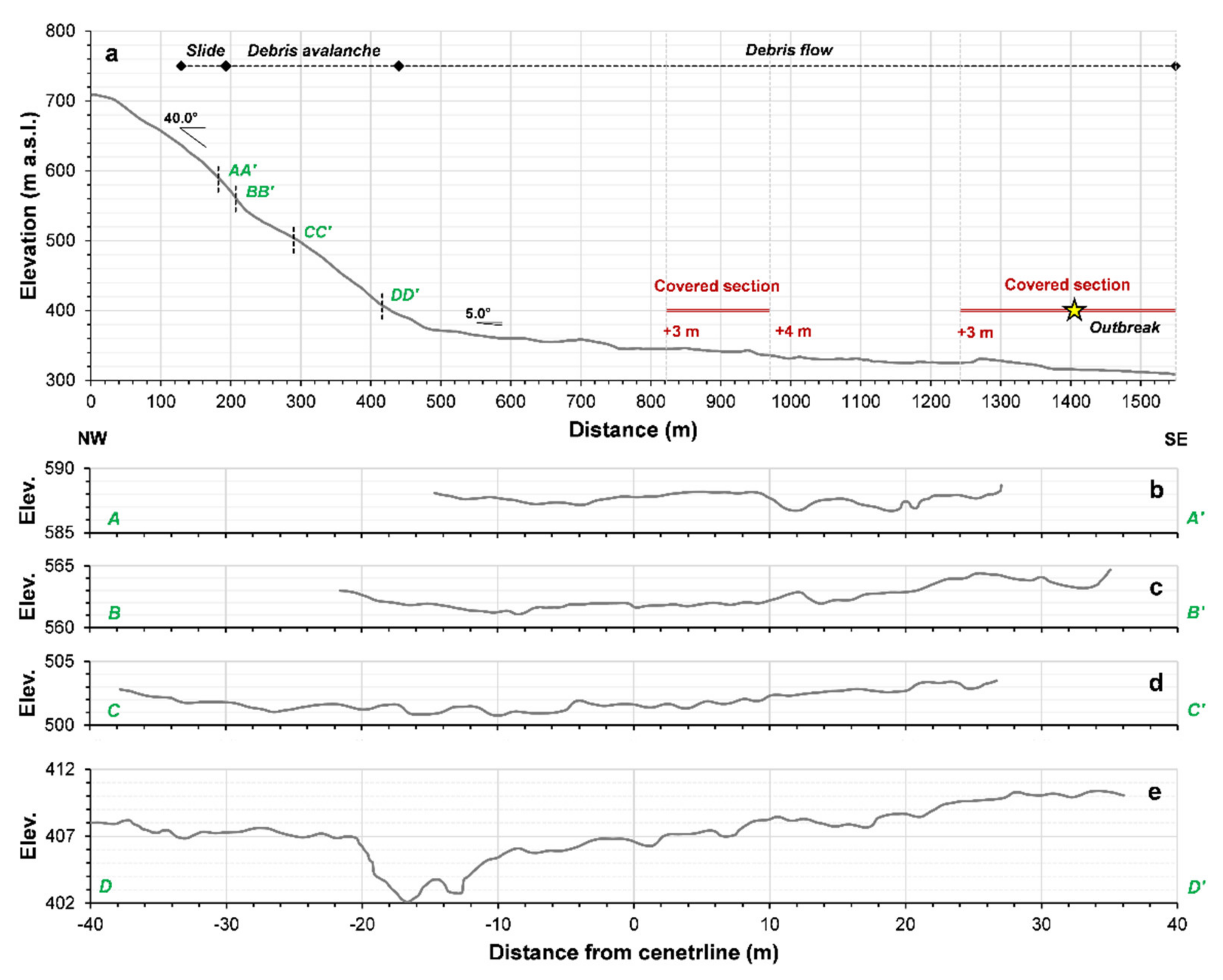
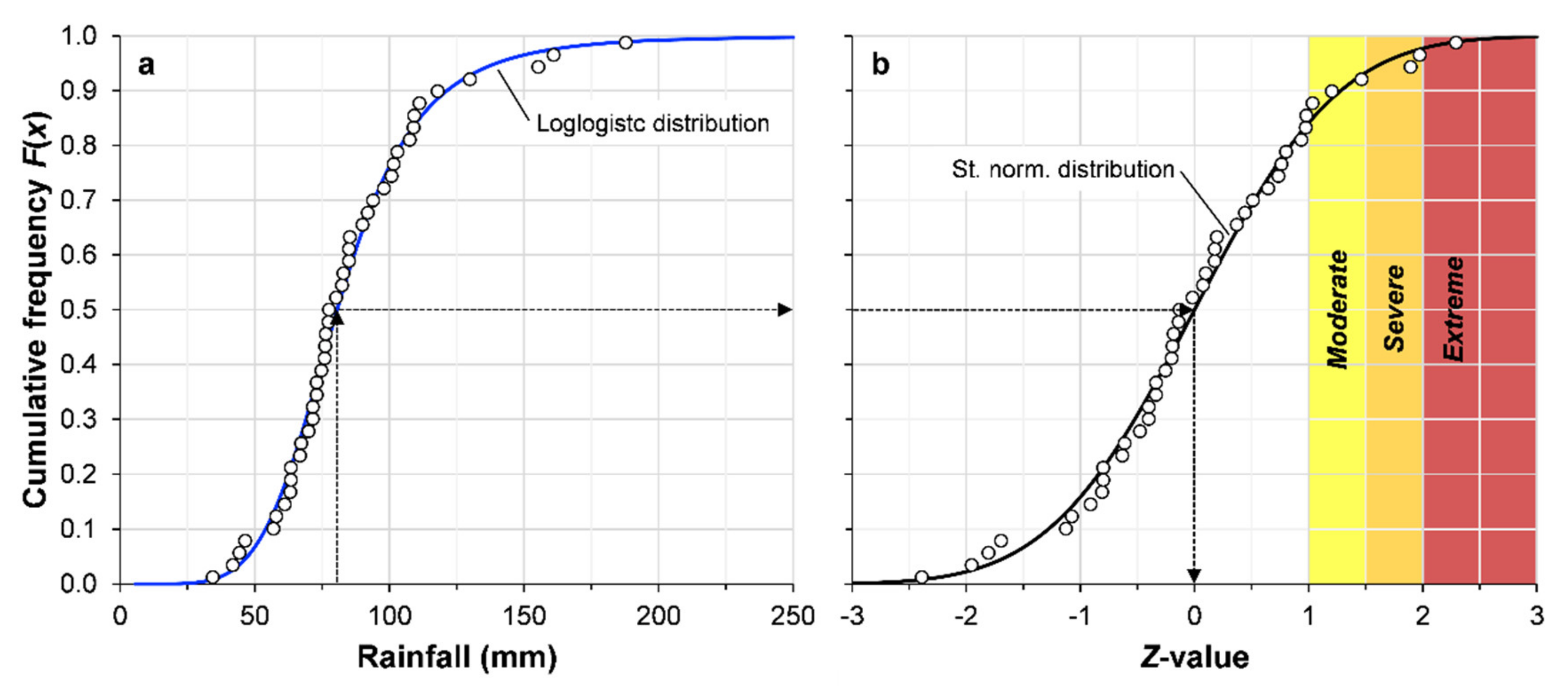
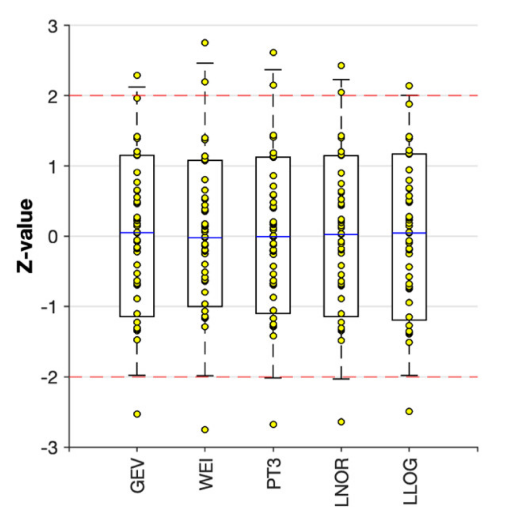
This study analyzed the powerful rainstorms that have occurred in S. Martino V.C. area, which has been hit by debris-flow events several times in the past. For this area, a suitable assessment of the magnitude of the rainstorms was performed based on a new approach, improving upon the procedure described by Fiorillo et al. [14]. The method is based on the frequency analysis of long time series (1966–2020 for the S. Martino V.C. rain gauge) of annual maxima of rainfall for precipitation durations of 1, 3, 6, 12 and 24 h. A criterion for selecting the most suitable probability distribution function for frequency analysis is also presented. The severity of the rainfall events was then estimated by transforming the data distribution into the standard normal distribution; therefore, the threshold value for defining an extreme event was established based on the assessment of the deviation of a specific rainstorm intensity from the long-term average conditions.

The assessment of the deviation of an observation from the mean value of the normalized time series is an unambiguous measure of the storm magnitude based on the historical records, independently from any trend in the time series. This procedure allows the ambiguity related to the definition of the return period to be overcome, which is one of the most used concepts in hydrology to measure the magnitude of an event.

The peculiar characteristics of the standardized time series, which are normally distributed and dimensionless, make them suitable also for further analyses. In particular, the trends of the standardized time series were investigated by least squares linear regression and tested by the t-test. In this way, the results obtained from the trend analysis of the time series of different rain gauges can be compared, given that these time series are now dimensionless and normally distributed.

2. Materials and Methods

2.1. Study Area

The town of S. Martino V.C. is located at 350 m a.s.l., along the Caudino Torrent, which drains a small but very steep basin, with elevation up to 1525 m a.s.l. and a catchment area of 6.4 km² upstream of the town. This catchment belongs to the northern slope of the Partenio Mts., located along the southern edge of the morpho-tectonic depression of the Caudina Valley (Figure 1). The relief consists of monoclines with a northeasterly dip direction and dips of 35°−70°, formed mainly by Cretaceous limestone sequences with bedding thicknesses ranging from decimeters to some meters [15].

Like the other surrounding karst massifs, these highlands are mantled by pyroclastic layers, predominantly air-fall tephra, deposited onto the karst bedrock surface, that are related to the volcanic activity of Vesuvius and the Phlegraean Fields [16].

The pyroclastic cover is generally composed of several irregular ashy pumiceous layers intercalated with buried soil, both with variable physical–mechanical properties. In particular, in the area of the Caudino Torrent catchment, remolded ash deposits can be observed along the steep slope upstream of S. Martino V.C. village. Figure 2 and

Table 1. Physical characteristics of the pyroclastic soil: Bw, weathered and remolded ash deposits; C, pumice level; Bt, weathered ash level; clay, silt, sand and gravel, fraction; γ_d, unit weight of dry soil; n, total porosity; n_eff, effective porosity (extracted from Reference [4]).

Layer	Clay (%)	Silt (%)	Sand (%)	Gravel (%)	γd (kN/m3)	n	neff
Bw	5	20	54	21	10.8	0.57	0.05–0.07
C	-	2	52	46	8.1	0.68	0.33–0.37
Bt	15	25	60	-	8.3	0.67	0.05–0.06

give a representative soil profile according to a standard soil taxonomy [17] and the corresponding physical properties. An important role is assumed by the lower pyroclastic level, which directly lies on the karstified limestone bedrock and infills the previous karst grooves along the slopes. This is a silty/clayey yellowish soil containing pumiceous elements and constitutes the basis along which landslide detachment occurs. This level has a maximum thickness at the base of the slope of up to a few meters and is almost constant along the steep slopes (0.5–1 m). It could be attributed (or ascribed) to the Campanian Ignimbrite (35,000 years B.P., following Reference [16]), which is widely present also in other areas of the Partenio Mts.

The sequences of pyroclastic layers covering the calcareous slopes are complex not only because of the local geometrical characteristics, but also because of their mechanical and hydrological features. The latter control the water retention and the water flow into soils and, thus, the conditions leading to landslide occurrence. Moreover, the steep slopes of these reliefs are a consequence of the features of the karst bedrock, which is characterized by a higher shear strength than the overlying pyroclastic mantle. Moreover, the karst bedrock favors the deep infiltration of the rainwater, limiting the runoff processes.

2.2. Hydrological Data and Climatic Features

The rainfall time series of the 1-, 3-, 6-, 12- and 24-h annual maxima were analyzed for several rain gauges, which were selected based on the length of the available time series and their location. In particular, the rain gauges have almost continuous data records, longer than 45 years, and are located close to the karst reliefs, which are mantled by pyroclastic deposits and have been hit by debris flows during the past (Figure 1).

Rainfall data were provided by the National Hydrographic and Oceanographic Service [11], up to 1999, and by the Multi-risk Functional Center of Civil Protection of the Campania Region [18] later.

For the S. Martino V.C. area, hourly, daily and monthly rainfall data are available starting from 1966. Initially, the rain gauge was located at 300 m a.s.l. and near the town. Since 2000, the rain gauge has been abandoned and the data have been recorded by a rain gauge located about 3.5 km south of the previous one, in the central sector of the Caudino Torrent catchment, at 757 m a.s.l.

The area is characterized by a Mediterranean climate: the dry-and-hot season lasts from June to September, while the wet-and-cool period lasts from October to May (Figure 3). The most intense rainfall (1 h) occurs in September and November; the long-duration rainfall (≥3 h) occurs in autumn/winter, while more evenly distributed rainfall events generally occur in spring [4].

To reconstruct the spatial distribution of the rainfall from the main storms that occurred around S. Martino V.C. (December 1968, December 1999 and December 2019), daily data were considered for more than one hundred rain gauges of the Campania network. The software tool QGIS v. 3.18 was used for the spatial interpolation of the rainfall data.

2.3. Historical Landslide Events and Debris-Flows Mapping

The area surrounding the S. Martino V.C. village has been hit by debris flows and floods several times in the past. The first documented historical news is related to the event of 2 October 1949, when heavy rainfall caused the flooding of the Caudino Torrent, which drains a small catchment located upstream of the S. Martino V.C. village, causing widespread damage. The storm of 1949 affected a wide area of the Campania region, and many catastrophic floods occurred in other places [19]. Although historical information is less detailed for this event in this area, no landslides appear to have occurred in 1949. By contrast, during the period of prolonged rainfall of 1962, which lasted for about two weeks, landslides occurred. Unfortunately, the latter were not mapped at that time, but some historical photographs have allowed them to be located. After the rainstorm of 16–20 December 1968, many landslides occurred along the carbonate slopes located east of the S. Martino V.C. village. Some of them caused debris flows which reached the village, and many people were evacuated. However, even the landslides of 1968 were not mapped at that time and no other details are available. In the night of 15 December 1999, prolonged and heavy rainfall triggered landslides, which struck a wide area of the Caudina Valley along the northern side of the Partenio ridge. The town of Cervinara was particularly affected [8]; six people died, and both houses and infrastructures were destroyed. During this storm event, some landslides also occurred in the area of S. Martino V.C., causing one death. The morphological signs of the 1999 landslides are still evident today along the slopes of this area. The recent landslides of December 2019 developed mainly in the area around S. Martino V.C. and occurred after prolonged–heavy rainfall, which also caused a flood and damage inside the urban area.

Historical photos, Google Earth multitemporal satellite images and unmanned aerial vehicle (UAV)-based remote-sensing methods were used for the landslide mapping. In particular, a historical photo showing the northeast slope of the Pizzone Mt. allowed us to map the main debris flow of the 1962 event (Figure 4).

The debris flows of December 1999 are well-known from several technical reports; the main debris flow, whose morphological signs are still evident today, was mapped based on Google Earth multitemporal satellite images. On the contrary, due to a lack of satellite images after the event of December 2019, UAV-based remote-sensing methods were used to map the 2019 debris flow. Moreover, a high-resolution Digital Surface Model (DSM) of the area was produced for this landslide. In particular, a DJI Phantom 4 Pro drone (SZ DJI Technology Co., Shenzhen, Guangdong, China) equipped with a digital RGB camera was used for photogrammetric surveying. Being a steep slope, the terrain-fallowing flight mode was used for taking images, allowing the UAV to adjust the flight height according to the terrain elevation during the image acquisition. Several flights were performed between January and February 2021, and they were finalized to find the optimal flight planning parameters for the UAV. The software Pix4Dmapper v. 4.5.6 [20] was then used for image matching, to obtain high-resolution digital orthophotos and a DSM of the landslide area.

2.4. Hydrological Analysis

2.4.1. Quantitative Estimation of Rainstorm Severity

In hydrology, the quantitative evaluation of the magnitude of an event, such as a river flood, hydrological and meteorological drought, storm, etc., is often based on the frequency analysis, which is the estimation of how often a specified event occurs [21].

The return period is probably one of the most used concepts in hydrology to measure the magnitude of an event and expresses its degree of rarity [22]. It is a function of the cumulative frequency, which is usually computed by fitting a parametric probability distribution function to the actual data.

Another way to quantify the magnitude of an event is to measure the deviation of a specific hydrological variable from the normal conditions observed over a specified time period. This simple method needs the observations to be normally distributed, and, therefore, it could not be used for hydrological variables, which are typically skewed. However, this disadvantage can be overcome by transforming the skewed distributions into normal distributions. In particular, this approach is generally used in calculating standardized indices, such as the Standardized Precipitation Index (SPI; [23]), which is used to monitor dry and wet periods [24]. The approach requires the choice and fitting of one or more univariate probability distribution functions. Once the optimal function is found, the cumulative frequency is transformed into the Z-value of the standard normal distribution, with mean μ = 0 and standard deviation σ = 1, by applying the inverse standard normal distribution function. Thus, the cumulative probability F(x), computed from a specific probability distribution function, was fixed equal to the cumulative probability of the standard normal distribution F(Z), as shown in the example in Figure 5.

$$F\left(x\right)\equiv F\left(Z\right)$$

(1)

$$F\left(Z\right)=\frac{1}{\sqrt{2\pi }}{{\displaystyle \int }}_{-\infty }^Z{e}^{\raisebox{1ex}{$-Z^2$}\!\left/ \!\raisebox{-1ex}{$2$}\right.}$$

(2)

where x represents the values of a random sample of finite size, drawn from a real-valued random variable X, describing the hydrological process under study.

Therefore, the magnitude of an event is represented by the number of positive or negative standard deviations; a positive or a negative Z-value indicates that the event magnitude is above or below the long-term mean of the time series, respectively. When analyzing the annual maximum values, hydrologists are interested in assessing the magnitude of the events located in the upper-tail of the distribution (positive Z-values) and, more specifically, in the extreme upper-tail. Based on the Z-value, an event is moderate if 1 ≤ Z < 1.5, severe if 1.5 ≤ Z < 2 and extreme if Z ≥ 2 [14]. The generic term “heavy” rainfall could refer to events with Z ≥ 1.5. Furthermore, the terms “short–heavy” and “prolonged–heavy” rainfall could refer to rainfall durations ≤ 6 h and >6 h, respectively.

In this study, the generalized extreme value (GEV), Weibull (WEI) Pearson Type III (PT3), lognormal (LNOR), and loglogistic (LLOG) probability distribution functions (

Table 2. Cumulative distribution functions F(x) and their parameters; Φ is the standard normal cumulative distribution function, while Γ(α) is the gamma function.

Distribution	F(x)	Parameters
Loglogistic	$F\left(x\right)={\left[1+{\left(\frac{\beta }{x-\gamma }\right)}^{\alpha }\right]}^{-1}$	α > 0
		β > 0
		γ ≤ x < +∞
Lognormal	$F\left(x\right)=\mathsf{\Phi }\left[\frac{\ln \left(x-\gamma \right)-\beta }{\alpha }\right]$	α > 0
		−∞ < β < +∞
		γ < x < +∞
Pearson Type III	$F\left(x\right)=\frac{1}{\beta \Gamma \left(\alpha \right)}{{\displaystyle \int }}_{\gamma }^x{\left(\frac{x-\gamma }{\beta }\right)}^{\alpha -1}\exp \left(-\frac{x-\gamma }{\beta }\right)dx$	α > 0
		β > 0
		γ ≤ x < +∞
Gen. extreme value	$F\left(x\right)=\exp \left\{\left.-{\left[1+\alpha \left(\frac{x-\gamma }{\beta }\right)\right]}^{-1/\alpha }\right\}\right.$	α ≠ 0
		β > 0
		$\mathrm{for} \alpha >0, x\ge \gamma -\beta /\alpha$
		$\mathrm{for} \alpha <0, x\le \gamma -\beta /\alpha$
Weibull	$F\left(x\right)=1-\exp \left[-{\left(\frac{x-\gamma }{\beta }\right)}^{\alpha }\right]$	α > 0
		β > 0
		γ ≤ x < +∞

) were chosen for the frequency analysis of 1-, 3-, 6-, 12-, and 24-h annual maximum rainfall time series recorded by the S. Martino V.C. rain gauge during the period 1966–2020, and by other rain gauges of the western–central sector of the Campania region (Figure 1). In particular, the three-parameter functional forms of these distributions were used, which are generalizations of the respective two-parameter functions and are more appropriate for analyzing the annual series of maximum values [25]. The three parameters of the distributions, i.e., the shape (α), the scale (β) and the location (γ) parameters, were estimated from the actual datasets by using the L-moment [21] and the maximum likelihood methods. A demo version of the EasyFit software v. 5.6 (MathWave Technologies) was used to estimate the probability distribution parameters.

Figure 5. (a) Transformation of the best-fitting distribution (three-parameter loglogistic distribution) into (b) a standard normal distribution. Actual data (white circles) are plotted by using the Gringorten formula [26]. The magnitudes of the rainstorms falling in the upper-tail part of the distributions (positive Z-values) are described by colors, where an event can be classified as moderate (1 ≤ Z < 1.5), severe (1.5 ≤ Z < 2) or extreme (Z ≥ 2).

Figure 5. (a) Transformation of the best-fitting distribution (three-parameter loglogistic distribution) into (b) a standard normal distribution. Actual data (white circles) are plotted by using the Gringorten formula [26]. The magnitudes of the rainstorms falling in the upper-tail part of the distributions (positive Z-values) are described by colors, where an event can be classified as moderate (1 ≤ Z < 1.5), severe (1.5 ≤ Z < 2) or extreme (Z ≥ 2).

2.4.2. Probability Distribution Function Selection

A major problem in the analysis of annual maximum rainfall is identifying a parametric probability distribution function that best represents the frequency of the data. The selection of the distribution function is a key decision in calculating both the return period (Tr) and the Z-value, as the selection of an inappropriate distribution may impart bias to the Tr and Z-value, exaggerating or minimizing the degree of rarity (Tr), or the magnitude (Z-value), of the observed phenomenon [27].

This problem has been widely discussed in the literature, and many methods have been proposed to allow hydrologists to choose the optimal functions [25,28,29,30]. The choice of a model to be used for statistical inference is often based on probabilistic hypotheses testing criteria. Commonly, the Kolmogorov–Smirnov and the Anderson–Darling tests are used. They are empirical distribution function goodness-of-fit tests, which measure the probability that a given random sample is drawn from a population with a continuous distribution function F(x) by testing the null hypothesis, H₀, at a specific level of significance, α. When parameters of the assumed distribution have to be estimated from the sample data, the critical values of the test statistics of the Kolmogorov–Smirnov and Anderson–Darling tests are difficult to find theoretically [31,32] and can be obtained only by time-consuming Monte Carlo simulations (e.g., see Reference [33]). However, even when critical values are known, the procedure has some limitations; in particular, the results could be ambiguous, as more than one probability distribution often passes the goodness-of-fit tests [34].

In this study, a method was proposed to select the appropriate probability model. According to this method, the quantiles of the standardized series, obtained by transforming the actual data, were compared to specific quantiles of the theoretical standard normal distribution. Based on the assumption that the quantiles of transformed time series should be equal to the theoretical quantiles of a standard normal distribution (in the hypothesis of perfect matching between the distribution fit and the observed data), the model that generates the smallest differences between computed and expected quantiles should be suitable for calculating robust standardized series, as it does not exaggerate or minimize the magnitude of the observed events.

The results were then graphically summarized by means of modified boxplots. These modifications take into account the features of a standard normal distribution. Different from a common boxplot [35], the upper and the lower boundaries of the box are the quantiles corresponding to probabilities of 0.841 and 0.159, which are equal to Z = 1 and Z = −1 for a standard normal distribution, respectively. The line inside the box identifies the median, which corresponds to a probability of 0.5 (Z = 0), and also corresponds to the mean value. The upper whisker extends from the upper boundary of the box up to the quantile corresponding to a probability of 0.977 (Z = 2), while the lower whisker extends from the lower boundary of the box up to the quantile corresponding to a probability of 0.023 (Z = −2). Values having probabilities greater than 0.977 and less than 0.023 represent extreme values and would correspond to Z-values greater than 2 and less than −2, respectively. Therefore, a perfect fit provides a median equal to zero (Z = 0), a box width between Z = 1 and Z = −1 and whiskers which extent up to Z = 2 and Z = −2. Thus, the performance of each distribution was estimated by summing the absolute values of the differences, |Δ|, between the computed (Z^c) and the expected (Z^e) quantiles, corresponding to probabilities of 0.977, 0.841, 0.5, 0.159 and 0.023:

$$\begin{array}{c}{\displaystyle \sum }\left|\Delta \right|=\left|Z_{0.977}^e-Z_{0.977}^c\right|+\left|Z_{0.841}^e-Z_{0.841}^c\right|+\left|Z_{0.5}^e-Z_{0.5}^c\right|+\left|Z_{0.159}^e-Z_{0.159}^c\right|\\ +\left|Z_{0.023}^e-Z_{0.023}^c\right|\end{array}$$

(3)

An example is shown in

Table 3. Z-values extracted from Figure 6 (6-h rainfall time series) for specific cumulative probabilities.

Probability	Z-Value
	Standard Normal Distribution	Generalized Extreme Value	Weibull	Pearson T. III	Lognormal	Loglogistic
0.977	+2	2.125	2.464	2.383	2.230	2.005
0.841	+1	1.151	1.079	1.125	1.146	1.171
0.500	0	0.050	−0.020	−0.054	0.024	0.045
0.159	−1	−1.144	−1.003	−1.117	−1.144	−1.194
0.023	−2	−1.979	−1.984	−2.048	−2.033	−1.981
Σ|Δ|		0.4908	0.5817	0.7271	0.5772	0.4341

and Figure 6, where the optimal fit is the loglogistic distribution for the 6-h rainfall time series of the S. Martino V.C. rain gauge.

2.4.3. Trend Analysis and Impact of Gaps on Trend Detection

A trend is a gradual change in a data series over time. Tests for trend detection can be classified as parametric and non-parametric; among the most widely used trend detection tests in hydrology, there are the least squares linear regression and the Mann–Kendall [36,37] tests. The non-parametric Mann–Kendall test only needs the data to be independent, while the parametric least squares linear regression test also requires the data to be normally distributed [38]. However, studies based on Monte Carlo simulations demonstrated that this parametric test is more powerful than the Mann–Kendall test for normally distributed data [39]. Therefore, if independence and distributional assumptions are satisfied, the least squares linear regression test should be preferred to the Mann–Kendall.

In this study, the least squares linear regression method was used to detect trends in rainfall time series of annual maxima recorded by the S. Martino V.C. rain gauge and another 10 rain gauges of the Western–Central Campania region, using the MATLAB R2019b software. It is important to highlight that these time series are skewed, however, the data transformation described in Section 2.4.1 allows us to satisfy the assumption about the normal distribution of the data series required by the least squares linear regression test. Furthermore, the standardization transforms all the data distributions into the standard normal distribution, whose values are dimensionless (Z-values), allowing the magnitude of the trends of different time series to be compared.

Using the least squares linear regression approach, the trend of a time series is described by the slope b of the regression line. The detected trend (parameter b) was considered statistically significant when the test statistic, t, defined as the ratio between the slope b and the associated standard error, was lower than a specific critical value. In particular, the null hypothesis of trend absence is rejected if the probability (p-value) associated to the statistic t, which follows the student’s t-distribution, was lower than the critical level α = 0.05 [40].

As the analyzed annual rainfall series of S. Martino V.C. contains gaps, their impact on the trend detection was analyzed by simulations. More precisely, their effects were investigated by generating random data from specific probability distribution functions to fill the data gaps. A total of 10,000 iterations were done for each rainfall time series; at each iteration, only gaps were filled with random data generated from the distribution functions which fit best to the actual data. The filled time series were then transformed into the Z-value of the standard normal distribution. Finally, the trend line slope (b_fill) and the associated test statistic (t_fill) were computed for every time series.

3. Results

3.1. Historical Events and the Landslides of December 2019

The main landslides of the area investigated in this study have affected the steep carbonate slopes of the Pizzone Mt. They are shown in Figure 7 and occurred in December 1962, December 1999 and December 2019. Landslides also occurred in December 1968 along the hill located east of the S. Martino V.C. village.

Based on rainfall data recorded by more than 100 stations of the Campanian rain gauge network, the isohyet maps of the 16–20 December 1968, 14–16 December 1999 and 19–23 December 2019 rainstorms were made by using the kriging method and are shown in Figure 8. For all three storm events, high rainfall intensities were observed in the area of the Partenio Mt. The 1968 rainstorm affected a wide area of the Campania region, where the sectors receiving the most rain (>400 mm in 5 days) were observed in the areas of the main karst reliefs (Miletto, Partenio, Cervialto and Lattari Mountains). For 1999, the areas with the heaviest rainfall (>300 mm in 3 days) were located in the areas of the Cervialto and Partenio Mts. For the 2019 event, the maximum rainfall intensities were observed on the Partenio Mts. (>400 mm in 5 days) and the Lattari Mts. (>300 mm in 5 days).

With regard to the main debris flow of December 2019 (Figure 7), from an elevation of about 630 m a.s.l., a pyroclastic body moved as a debris slide moved over a surface with a dip of about 40°. In general, these high slope angles are connected to the features of the karst bedrock, which is characterized by a higher shear strength than the pyroclastic layer. Moreover, the karst bedrock favors the deep infiltration of the rainwater.

The sliding surface had to be located at the top of the lower pyroclastic level (ignimbrite deposit; Figure 2), where the mean thickness in the scar zone was estimated to be about 1 m. In situ surveys allowed the local conditions of the detachment zone (Figure 9c,d) to be verified, where the karst substratum outcrops with an open vertical joint through which water flow could occur during intense storms.

Above the main scar, many trees fell forward due to other debris slides, which did not evolve into avalanche types and stopped after a few meters, as in many other zones of the steep slope (Figure 10). Practically, many debris slides occurred, but locally only one evolved into a debris avalanche (Figure 10). Following the detachment at 630 m a.s.l., the landslide progressively involved the entire pyroclastic mantle of the slope, including the vegetation, which consisted mainly of chestnut trees. Downslope, the thickness of the pyroclastic mantle does not increase until the slope gradually decreases towards the torrent. As for other similar landslides in the Campania area, this phase of the movement is particularly notable, as it gives the landslide the characteristics of a debris avalanche, which usually has a considerable velocity. The rumble heard by the local population in the late afternoon of 21 December 2019 can be associated with this phase.

Figure 11 shows that the sliding surface has a slightly concave shape with a highly irregular profile due to the karstification of the bedrock. This would suggest that the thickness of the pyroclastic cover is not constant along the slope, making it difficult to accurately estimate the volume of the material involved in the movement, which has been estimated to be between 15,000 and 20,000 m³.

Figure 11. (a) Longitudinal topographic profile along the landslide area, showing the types of movement and slope. Covered sections of the Caudino Torrent and flow thickness (red numbers) are also shown. (b–e) Topographic profiles from the UAV survey (the location of the traces AA’, BB’, CC’ and DD’ is shown in Figure 9).

Figure 11. (a) Longitudinal topographic profile along the landslide area, showing the types of movement and slope. Covered sections of the Caudino Torrent and flow thickness (red numbers) are also shown. (b–e) Topographic profiles from the UAV survey (the location of the traces AA’, BB’, CC’ and DD’ is shown in Figure 9).

At the base of the slope and after considerable expansion (Figure 9), the landslide material probably caused a temporary filling of the valley floor and was progressively drained by the Caudino Torrent, which locally crosses the urban stretch with several covered segments built during different historical periods (Figure 7 and Figure 11). During its passage, along the Caudino Torrent, the phenomenon evolved into a hyper-concentrated streamflow due to dilution (sensu [41]). During the in situ surveys, the height that the flow reached once it was channeled in the Caudino Torrent was measured (Figure 7, Figure 11 and Figure 12). An occlusion of the torrent in its lowest covered segments, probably caused by the accumulation of the debris and the tree trunks, caused the outbreak of the covered torrent segment inside the town shortly after 19:00. Other minor landslides occurred locally during the storm of December 2019. In particular, another landslide occurred on the eastern side of the Pizzone Mt., 1 km southeast from the main landslide, at about 635 m a.s.l., and blocked the local Mafariello road.

3.2. Severity of Rainstorms and Trend Analysis

The best-fitting probability distributions were chosen for the time series (1, 3, 6, 12 and 24 h) of the R1 rain gauges, and of the other ten considered rain gauges, according to the method described in Section 2.4.2. The best-fit functions for each time series are shown in

Table 4. Best-fit probability distribution functions used for computing standardized time series of annual maxima of rainfall. Five different probability distributions were considered: generalized extreme value (GEV), Weibull (WEI), Pearson Type III (PT3), lognormal (LNOR) and loglogistic (LLOG).

Station	No. of Data	1 h	3 h	6 h	12 h	24 h
R1	55	LNOR	LLOG	LLOG	LLOG	LLOG
R2	72	WEI	PT3	LNOR	LNOR	LLOG
R3	48	GEV	LNOR	LNOR	LLOG	LLOG
R4	57	PT3	LLOG	LLOG	LLOG	LLOG
R5	80	GEV	PT3	LNOR	LNOR	LLOG
R6	73	LLOG	LLOG	LLOG	LLOG	LLOG
R7	86	WEI	GEV	LLOG	LLOG	LLOG
R8	44	LNOR	WEI	LNOR	LLOG	LLOG
R9	67	LNOR	GEV	LLOG	LLOG	LNOR
R10	71	LLOG	LNOR	LNOR	LNOR	LNOR
R11	56	GEV	LLOG	LLOG	LLOG	GEV

S. Martino V.C. (R1), Avellino (R2), Montemarano (R3), Sarno (R4), Giffoni Vallepiana (R5), Caposele (R6), Senerchia (R7), Massa Lubrense (R8), Cava De’ Tirreni (R9), Salerno (R10), Baronissi (R11).

. The computed probabilities were then transformed into the Z-value of the standard normal distribution to obtain standardized annual maximum rainfall time series.

Figure 13 shows the frequency distributions selected for R1 (Figure 13a) and their transformation into the Z-value of the standard normal distribution (Figure 13b).

Figure 14 shows the standardized time series of R1. For the 1-h time series, severe rainfall (1.5 ≤ Z < 2) occurred in 1981, 2003 and 2014, while extreme rainfall (Z ≥ 2) occurred in 2018; however, no landslides occurred in these years. For the 3-h time series, severe rainfall occurred in 2014 and 2019, while extreme rainfall occurred in 1997. However, no landslides occurred in 2014 or 1997. For the 6-h time series, severe and extreme rainfalls occurred in 1997 and 2019, respectively. The storm events of December 1968, December 1999 and December 2019 that caused landslides show the highest magnitude only in the cases of 12- and 24-h rainfall intensities. In particular, for the 12-h time series, the 1968 and 1999 events are severe and show Z-values close to 2, while the 2019 event is extreme. For the 24-h time series, all three events are extreme.

Table 5. Actual maximum rainfall intensities, h (mm), of the three storm events which caused the landslides of S. Martino V.C.; the Z-values (standard deviations, σ) of the events were computed from three-parameter lognormal distribution for the 1-h rainfall and from three-parameter loglogistic distribution for the 3-, 6-, 12- and 24-h rainfall series.

Storm	Rainfall	1 h	3-h	6 h	12 h	24 h
Dec-1968	h (mm)	30.0	60.0	100.0	161.0	275.6
	Z-value (σ)	0.017	0.956	1.393	1.972	2.324
		-	-	Moderate	Severe	Extreme
Dec-1999	h (mm)	19.0	53.4	93.0	155.4	253.0
	Z-value (σ)	−1.397	0.580	1.224	1.893	2.173
		-	-	Moderate	Severe	Extreme
Dec-2019	h (mm)	37.4	92.2	147.8	187.8	248.8
	Z-value (σ)	0.755	1.998	2.138	2.292	2.142
		-	Severe	Extreme	Extreme	Extreme

shows the severity of the 1968, 1999 and 2019 storms in terms of rainfall amount h (mm) and Z-value (standard deviations, σ). Based on this analysis, the landslides in the study area appear to be related to heavy rainfall having a duration ≥ 12 h. On the contrary, intense and short-duration rainfall (1-, 3- and 6-h) should not be able to induce landslides, as in the case of 1981, 1997 and 2014 events, which are severe events associated with Z-values much greater than 1.5.

The least squares linear regression method was the applied to assess the parameter b of the trend lines and its significance for the analyzed time series (Figure 14). As can be seen, positive trends were found in all cases, indicating a general increase in the annual maximum intensities of rainfall since 1966. The 1- and 3-h series show the highest slope values of the trend line, which are 0.0237 and 0.0224 σ/year, respectively. The lowest value (0.008 σ/year) was found for the 12-h series. At a significance level of α = 0.05, only the 1- and 3-h series show statistically significant trends (p-value < 0.05). On the contrary, trends in the 6-, 12- and 24-h series were not statistically significant (p-value > 0.05).

Figure 15 shows the results obtained from the trend analysis of the filled time series using boxplots [35] for the R1 rain gauges. Synthetic data were generated from lognormal and loglogistic distributions. As shown by the figure, all filled time series give positive trend values, indicating that data gaps do not affect the sign of the trends. For all series, the slope values estimated from the transformed actual data (Figure 14) are above the 50th percentile (Figure 15a).

Furthermore, we note that data gaps do not affect the trend significance. In particular, the 1- and 3-h series show statistically significant trends (t-statistic > 2.005, p-value < 0.05; Figure 14a,b). For the 1- and 3-h time series with filled gaps, the null hypothesis of trend absence is rejected in 98% and 95% of the cases, respectively (Figure 15b). The time series of the 12- and 24-h rainfall series have no statistically significant trends (t-statistic < 2.005, p-value > 0.05; Figure 14d,e). The same occurs for the time series with filled gaps (Figure 15b). The 6-h time series does not show a statistically significant trend (Figure 14c). For the 6-h time series with filled gaps, the detected trends are not statistically significant in almost 85% of the cases (Figure 15b).

The trends detected in the time series of the S. Martino V.C. rain gauges (R1) were compared with the trends of other rain gauges of the western–central sector of Campania. These rain gauges are located close to the karst massifs of the Lattari and Partenio-Sarno Mts. Both massifs have been hit by debris flows in the past. Both positive and negative linear trends were detected in the standardized time series (

Table 6. Results of the least squares linear regression test applied to the time series of annual maxima of rainfall of the 11 considered rain gauges. Elevation (in m a.s.l.) of the rain gauge, the starting year of the time series and the number of available data are reported in table. The parameter b (in σ/year, where σ is the standard deviation) is the slope of the regression line; statistically significant trend line slopes (p-value < 0.05) are shown in bold.

Station	Elevation	Beginning	No. of Data	Trend	1 h	3 h	6 h	12 h	24 h
R1	751	1966	55	b	0.0237	0.0224	0.0154	0.0075	0.0116
				p-value	0.0064	0.0103	0.0823	0.4116	0.2096
R2	360	1949	72	b	0.0134	0.0086	0.0036	−0.0009	0.0002
				p-value	0.0238	0.1535	0.5557	0.8865	0.9720
R3	865	1973	48	b	0.0145	0.0164	0.0103	0.0115	0.0040
				p-value	0.1634	0.1295	0.3442	0.2855	0.7205
R4	124	1964	57	b	0.0169	0.0133	0.0096	0.0045	−0.0034
				p-value	0.0515	0.1337	0.2782	0.6090	0.7020
R5	980	1941	80	b	0.0065	0.0052	0.0019	0.0026	0.0025
				p-value	0.2173	0.3324	0.7195	0.6304	0.6431
R6	428	1948	73	b	0.0169	0.0168	0.0068	0.0095	0.0110
				p-value	0.0090	0.0110	0.3169	0.1584	0.0976
R7	578	1935	86	b	0.0140	0.0044	0.0012	0.0007	0.0024
				p-value	0.0017	0.3344	0.7985	0.8893	0.6043
R8	385	1977	44	b	−0.0156	−0.0111	−0.0116	−0.0087	−0.0116
				p-value	0.2072	0.3306	0.3510	0.4837	0.3437
R9	195	1954	67	b	−0.0002	−0.0106	−0.0156	−0.0177	−0.0153
				p-value	0.9752	0.1028	0.0154	0.0055	0.0152
R10	13	1950	71	b	0.0011	−0.0003	−0.0027	−0.0011	0.0013
				p-value	0.8541	0.9553	0.6524	0.8527	0.8222
R11	226	1965	56	b	−0.0035	−0.0098	−0.0072	−0.0059	−0.0079
				p-value	0.6892	0.2643	0.4125	0.5017	0.3566

S. Martino V.C. (R1), Avellino (R2), Montemarano (R3), Sarno (R4), Giffoni Vallepiana (R5), Caposele (R6), Senerchia (R7), Massa Lubrense (R8), Cava De’ Tirreni (R9), Salerno (R10), Baronissi (R11).

). In particular, rain gauges of the Lattari Mts. (R8, R9, R10 and R11) have negative trends in the majority of the cases. However, statistically significant trends were detected for R9 only. The rain gauges around the Partenio-Sarno Mts. are characterized by no significant positive trends in most cases.

4. Discussions

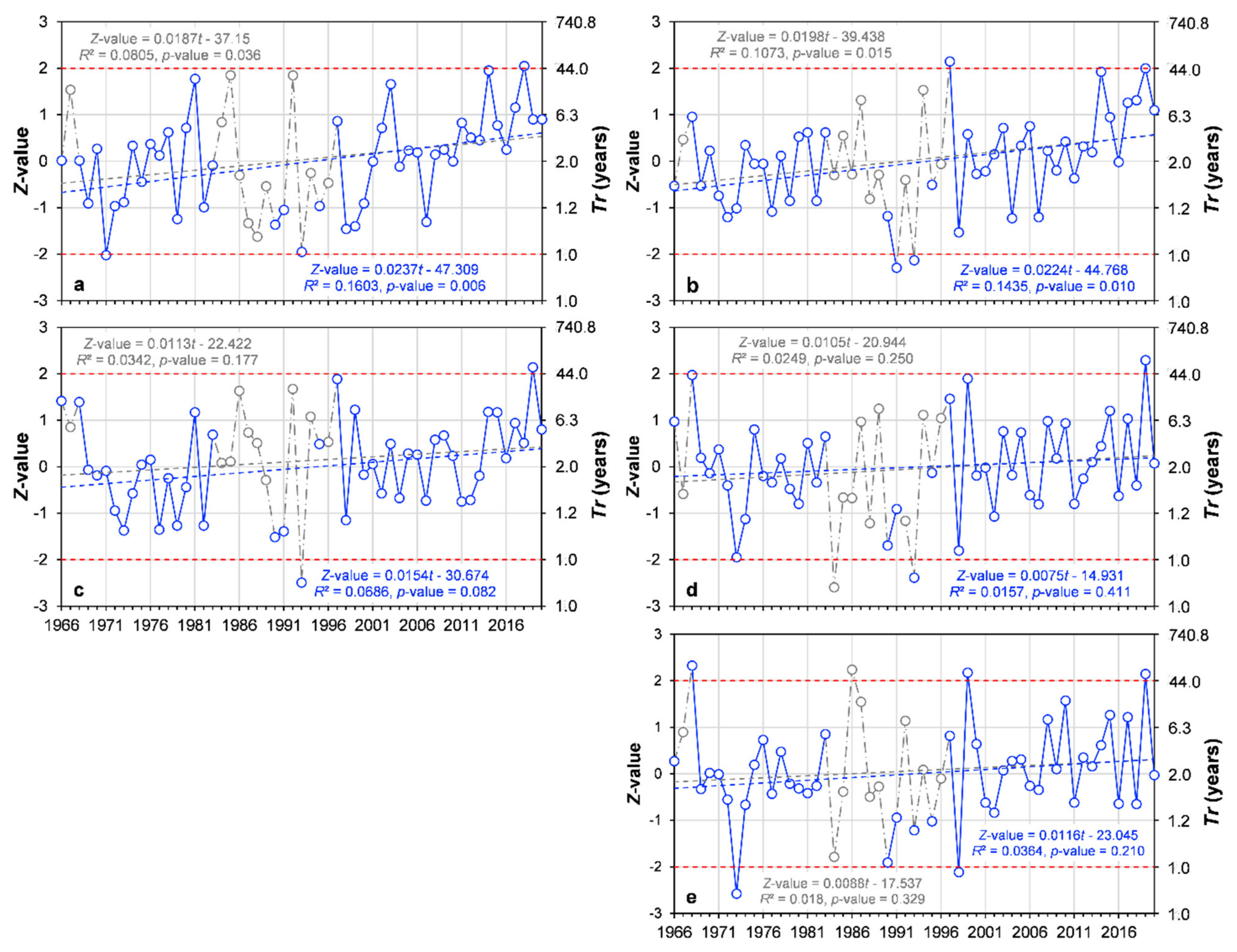
Trend analysis has shown a general shift toward more intense rainfall in all of the time series of the R1 rain gauge. When considering rainfall durations of 1 and 3 h, these trends are statistically significant. On the contrary, trends in 6-, 12- and 24-h time series are not statistically significant for R1. In addition, the heaviest rainstorms (1968, 1999 and 2019) appear almost evenly distributed over time (Figure 14d,e).

Significant positive linear trends were also found for the Avellino (R2), Caposele (R6) and Senerchia (R7) rain gauges, for the 1-h time series. However, it should be noted that the high value of the trend line slope b found for the 1-h and 3-h time series of S. Martino V. Caudina (R1) could be influenced by the shift of the rain gauge, which occurred in 2000. The rain gauge was moved about 3.5 km from its initial position, from a location close to the outlet of the Caudino Torrent catchment (300 m a.s.l.), to the central sector of the catchment (751 m a.s.l.). Even if this could have altered the homogeneity of the time series, the two records (before and after 2000) can be considered as belonging to a single station. In fact, the analyses provided no statistically significant trends for the 6-, 12- and 24-h series of R1. The absence of significant trends in the 6-, 12- and 24-h rainfall time series of the R1 rain gauge appears to be supported by the results of trend analysis of the other rain gauges, where no statistically significant positive trends were detected in all cases. As discussed below, main attention must be given to 12- and 24-h rainfall events, which appear to be the most critical rainstorm durations for debris-flow initiation in this area.

In general, the absence of statistically significant increasing trends in the 6-, 12- and 24-h rainfall time series does not seem to be related to the length of the analyzed records. In fact, this behavior was also observed in the longest analyzed time series, which are those recorded by the R2 (1949–2020), R5 (1941–2020), R6 (1948–2020) and R7 (1935–2020) rain gauges.

The absence of significant trends found for the 6-, 12- and 24-h time series of the rain gauges of the Campania appears to be in line with that found in other areas of Southern Italy; in contrast, 1- and 3-h rainfall time series have significant positive trend more frequently.

Libertino et al. [42] assessed the presence of regional trends in the magnitude of annual rainfall maxima for precipitation durations of ≤24 h in Italy. Their analysis was limited to the period 1928–2014 and focused mainly on five regions of the Italian Peninsula. The authors underlined that the rainfall events with durations ≤ 24 h are characterized by large spatial heterogeneities, with a clear trend in rainfall time series that is not able to be detected at the country-scale. However, they recognized an increase in the rainfall severity for all durations in the northeastern part of the country and a decrease in the southern extreme of the peninsula (Calabria region).

Caporali et al. [43] provided a review of the studies on precipitation trends detected in Italy. However, many of the reviewed works analyzed time series which do not consider the rainfall data of the last decade. For Southern Italy, Arnone et al. [44] found statistically significant positive trends in the 1-h maximum annual rainfall time series only in 14% of the analyzed rain gauges; for 3-, 6- and 12-h durations, positive trends were detected at about 4–6% of the stations; for the 24-h duration events, no positive trends were found.

Bonaccorso and Aronica [45] obtained similar results. They investigated the temporal changes in the 1-, 3-, 6-, 12- and 24-h annual maxima of rainfall in Sicily. Only a few rain gauges, mainly located along the northern coast of Sicily, exhibited statistically significant positive trends, with the time series analyzed by the authors covering the period which spanned from 1928 to 2009.

Polemio and Lonigro [46] analyzed the annual maximum time series of the 1-, 3-, 6-, 12- and 24-h rainfall, collected from several rain gauges of the Apulia from 1921 to 2002. They detected positive and negative statistically significant trends only in a few time series. Generally, less than the 6.5% of the 1- and 3-h rainfall time series analyzed by the authors had statistically significant positive trends, while the 6-, 12- and 24-h rainfall time series had statistically significant trends in less than 3.5% of the cases.

Regarding other parts of the Italian Peninsula, Gentilucci et al. [47] analyzed the trends in maximum annual rainfall recorded by 128 rain gauges from 1921 to 2017 in the Marche region (Central Italy). They found that the growth of extreme precipitation events is significant in the southern part of the region, which is characterized mainly by a typical Mediterranean climate.

It has to be noted that the trend analysis was carried out on the standardized time series. In addition, the use of the Z-value for describing the magnitude of a rainstorm allows us to overcome the ambiguity related to the definition of the return period, especially under a climate change condition. This definition is widely debated in the literature, as it implicitly contains an indication of the future recurrence of events. The return period is generally used to provide the expected recurrence of an event; this use is formally correct, but possibly misleading, because the probability associated with an event within a time series actually is the probability of observing that event each year [22]. Instead, the Z-value remains fixed on the observed data series and would not provide any indication regarding the recurrence of these events in the future. For example, an event with a return period of 100 years means that it occurs statistically every 100 years, which is potentially a misleading result when the stationary of the time series cannot be guaranteed. For this reason, the use of the Z-value overcomes considerations about the stationarity of the time series, which is a debated topic in the literature (cf. References [48,49]). The Z-value, which is applied under the above-described procedure, would be an unambiguous measure of the storm magnitude based on historical records, independently from any trend in the time series. After the transformation of the observations, the Z-value provides an unbiased deviation from the mean value of the time series.

Table 7. S. Martino V.C. rain gauge (R1): actual maximum rainfall intensities h (mm) and Z-values of the storms of the historical series (1966–2020) characterized by hourly maxima falling in the severe (1.5 ≤ Z < 2) and extreme categories (Z ≥ 2).

Storm Date	Landslides	Rainfall	1 h	3 h	6 h	12 h	24 h
18-Dec-1968	Yes	h (mm)	30.0	60.0	100.0	161.0	275.6
		Z-value	-	-	-	1.972	2.324
7-Dec-1981	No	h (mm)	50.0	54.0	91.0	94.0	94.0
		Z-value	1.772	-	-	-	-
12-Nov-1997	No	h (mm)	38.6	99.6	127.6	130	139.2
		Z-value	-	2.144	1.885	-	-
15-Dec-1999	Yes	h (mm)	19.0	53.4	93.0	155.4	253.0
		Z-value	-	-	-	1.893	2.173
3-Jun-2003	No	h (mm)	48.4	55.6	55.6	55.6	55.6
		Z-value	1.656	-	-	-	-
9-Nov-2010	No	h (mm)	28.6	51.0	65.6	107.6	187.6
		Z-value	-	-	-	-	1.570
14-Jul-2014	No	h (mm)	52.6	88.8	91.4	92.0	93.4
		Z-value	1.954	1.924	-	-	-
17-Apr-2018	No	h (mm)	54.0	68.0	71.6	71.6	71.6
		Z-value	2.049	-	-	-	-
21-Dec-2019	Yes	h (mm)	37.4	92.2	147.8	187.8	248.8
		Z-value	-	1.998	2.138	2.292	2.142

shows all heavy rainfall events (Z ≥ 1.5) of the time series, split into severe (1.5 ≤ Z < 2) and extreme (Z ≥ 2) categories for the R1 rain gauge. Severe and extreme storms characterized by a short–heavy rainfall (1-, 3- and 6-h) occurred in 1981, 1997, 2003, 2014 and 2018. In all of these cases, no landslides occurred. The December 1968, 1999 and 2019 storm events, which caused landslides in the area, showed values of Z close to or higher than 2 and represent the heaviest events of the time series when 12- and 24-h rainfall intensities are considered. Moreover, for the 24-h rainfall, all three storms are extreme (Z ≥ 2).

Taking into account the information in Table 7, it appears that short–heavy rainfall (Z ≥ 1.5 for a duration ≤ 6 h) would not cause landslides; that is, it is statistically improbable that short–heavy rainfall events could cause debris flows under these climate conditions in this area. 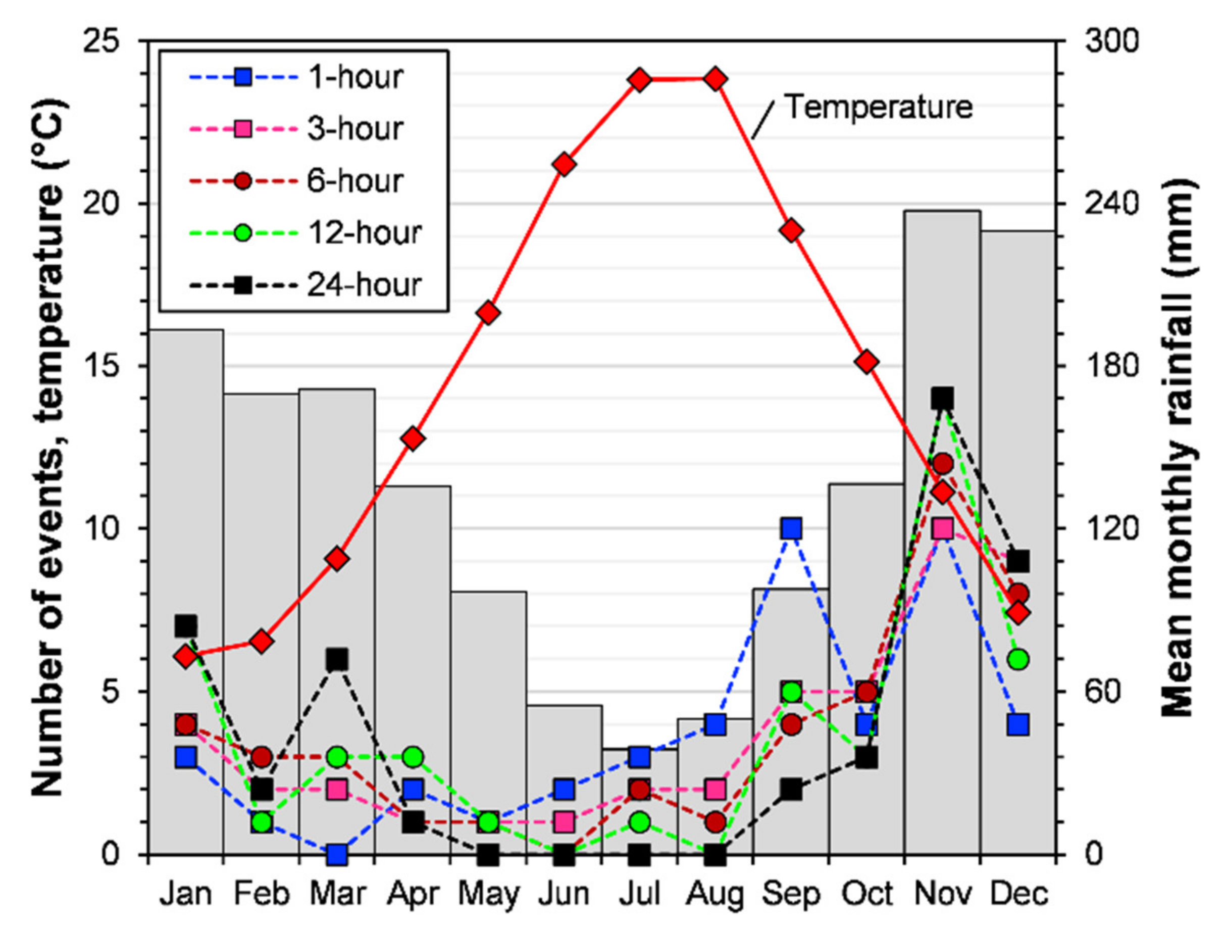Here, short–heavy rainfall (i) generally occurs during the beginning of the rainy season (September–November period, Figure 3), when rain water is partially retained as soil moisture [4], and (ii) could favor runoff processes along steep slopes. On the other hand, a prolonged–heavy rainfall (Z ≥ 1.5 for a duration > 6 h) would cause landslides (Table 7). In this area, the heaviest rainstorms of 12- or 24-h duration occur in December, when the soil moisture has generally reached its highest value (field capacity) [4], and it is useful to develop positive pore pressure or deep infiltration. Furthermore, the rainfall which occurs during December more easily reaches the ground surface, as they are not retained by the leaves of the chestnut trees, which fall in October/November.

For a 12-h duration event, the Z-value is between 1.46 (maximum Z-value of the 12-h rainfall which failed to induce landslides, November 1997) and 1.89 (minimum Z-value of the 12 h which induced landslides), corresponding to 130.0 and 155.4 mm of rain, respectively. For a 24-h duration event, the Z-value is between 1.57 (maximum Z-value of the 24-h rainfall which failed to induce landslides, November 2010) and 2.14 (minimum Z-value of the 24 h which induced landslides), corresponding to 187.6 and 248.8 mm of rainfall, respectively.

As is well-known, the initiation of debris flows is a combination of a powerful storm and a certain amount of antecedent rainfall [4,50]. In particular, the previous weather conditions directly influence the soil water content, which can be considered the final factor controlling the landslide initiation, as it directly affects the shear strength of the pyroclastic layer [4,8]. Since the soil is subjected to rainwater infiltration and evapotranspiration, the soil water content varies over the year according to the seasonal characteristics of rainstorms and temperature.

5. Conclusions

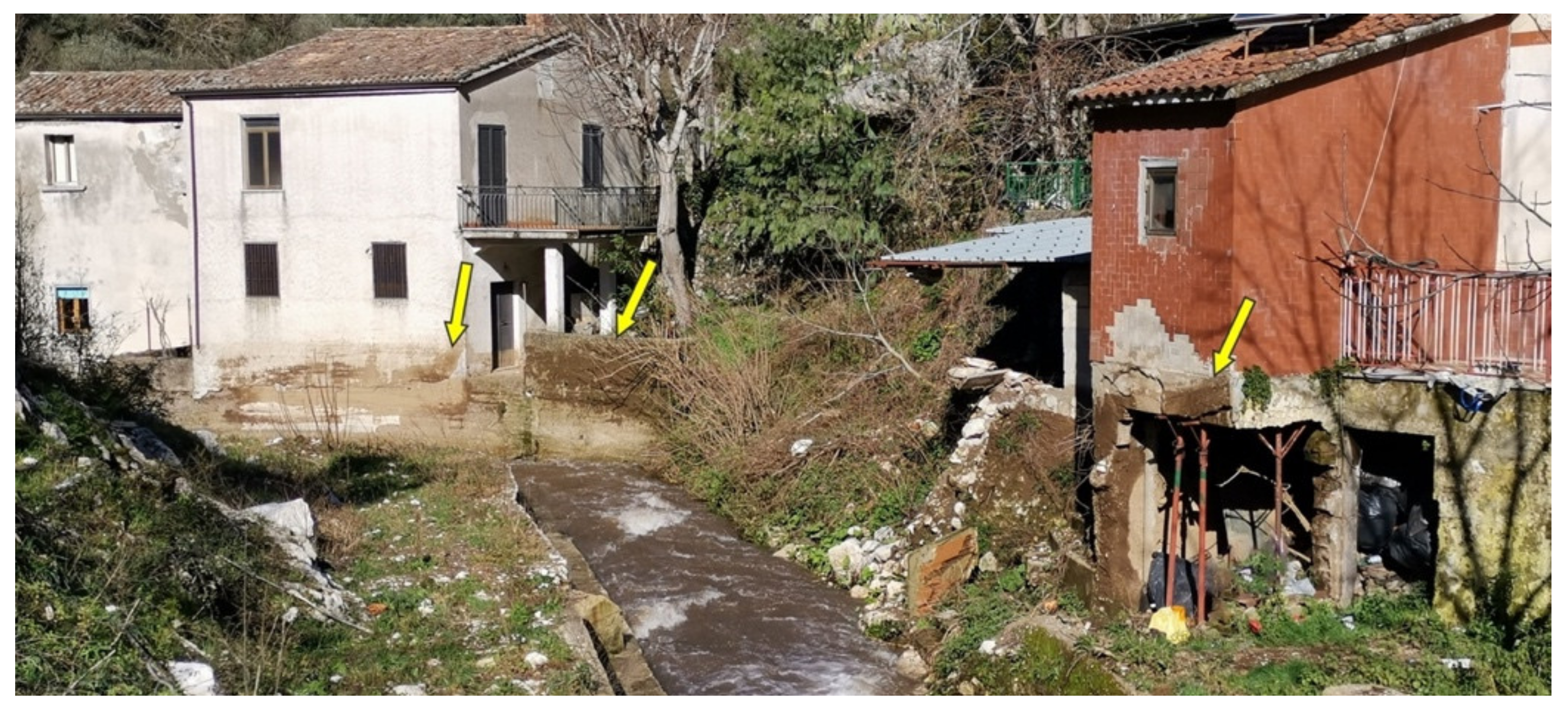
This case study focused on a sector of the Partenio Mts., where rainfall represents a main source of risk for urban settlements, as it was the driver of the catastrophic floods and the debris flows which have hit the area many times in the past. Part of the research dealt with the chronological reconstruction of the debris-flow events through historical photographs and newspapers, rainfall records and local testimonials. This is generally a difficult task, because, as well as for many areas of the Campania region, hydrological data are often missing, and time series are discontinuous. Moreover, the geomorphological processes and the regrowth of vegetation rapidly erase the topographic signs left by minor landslides along the slopes. Despite these difficulties, the results obtained in terms of the recurrence of landslide events make this area a further key location for studying these phenomena in Campania.

A new method to estimate the magnitude of rainfall events has been described in this work. It is based on the use of the Z-value of the standard normal distribution as a measure of the deviation from the mean value, which represents the long-term normal conditions. As the Z-value remains fixed on the observed data series, it does not provide any indications about the recurrence of the future events and appears as an unambiguous measure of the power of a storm.

Since the standardized time series are normally distributed, the use of the least squares linear regression test appears more suitable to detect trends. In addition, standardized data are dimensionless, and this allows us a better comparison between the slope of the trend lines of different time series (1, 3, 6, 12 and 24 h) and between time series recorded at different rain gauges.

Our findings indicate that the historical debris flows which have affected the S. Martino V.C. area in recent times were related to severe and extreme rainfall events having durations ≥ 12 h, as no landslide occurred for powerful rainfall of shorter durations (≤6 h). Moreover, significant changes in the intensity of the rainfall events were not observed during the time. In particular, it was found that the intensity of the rainstorms of a duration ≥ 6 h is not increasing.

References

1. Calcaterra, D.; Santo, A. The January 10, 1997 Pozzano landslide, Sorrento Peninsula, Italy. Eng. Geol. 2004, 75, 181–200. [Google Scholar] [CrossRef]
2. Guadagno, F.M.; Forte, R.; Revellino, P.; Fiorillo, F.; Focareta, M. Some aspects of the initiation of debris avalanches in the Campania Region: The role of morphological slope discontinuities and the development of failure. Geomorphology 2005, 66, 237–254. [Google Scholar] [CrossRef]
3. Fiorillo, F.; Guerriero, L.; Capobianco, L.; Pagnozzi, M.; Revellino, P.; Russo, F.; Guadagno, F.M. Inventory of Vietri-Maiori landslides induced by the storm of October 1954 (southern Italy). J. Maps 2019, 15, 530–537. [Google Scholar] [CrossRef]
4. Fiorillo, F.; Wilson, R.C. Rainfall induced debris flows in pyroclastic deposits, Campania (southern Italy). Eng. Geol. 2004, 75, 263–289. [Google Scholar] [CrossRef]
5. Galeandro, A.; Šimůnek, J.; Simeone, V. Analysis of rainfall infiltration effects on the stability of pyroclastic soil veneer affected by vertical drying shrinkage fractures. Bull. Int. Assoc. Eng. Geol. 2013, 72, 447–455. [Google Scholar] [CrossRef] [Green Version]
6. De Vita, P.; Napolitano, E.; Godt, J.; Baum, R. Deterministic estimation of hydrological thresholds for shallow landslide initiation and slope stability models: Case study from the Somma-Vesuvius area of southern Italy. Landslides 2012, 10, 713–728. [Google Scholar] [CrossRef]
7. Cuomo, S.; Masi, E.B.; Tofani, V.; Moscariello, M.; Rossi, G.; Matano, F. Multiseasonal probabilistic slope stability analysis of a large area of unsaturated pyroclastic soils. Landslides 2021, 18, 1259–1274. [Google Scholar] [CrossRef]
8. Comegna, L.; Damiano, E.; Greco, R.; Olivares, L.; Picarelli, L. The Hysteretic Response of a Shallow Pyroclastic Deposit. Earth Syst. Sci. Data 2021, 13, 2541–2553. [Google Scholar] [CrossRef]
9. Greco, R.; Comegna, L.; Damiano, E.; Marino, P.; Olivares, L.; Santonastaso, G.F. Recurrent rainfall-induced landslides on the slopes with pyroclastic cover of Partenio Mountains (Campania, Italy): Comparison of 1999 and 2019 events. Eng. Geol. 2021, 288, 106160. [Google Scholar] [CrossRef]
10. Napolitano, E.; Fusco, F.; Baum, R.L.; Godt, J.W.; De Vita, P. Effect of antecedent-hydrological conditions on rainfall triggering of debris flows in ash-fall pyroclastic mantled slopes of Campania (southern Italy). Landslides 2015, 13, 967–983. [Google Scholar] [CrossRef]
11. Annali Idrologici. Available online: http://www.acq.isprambiente.it/annalipdf/ (accessed on 25 March 2021).
12. Cascini, L.; Cuomo, S.; Guida, D. Typical source areas of May 1998 flow-like mass movements in the Campania region, Southern Italy. Eng. Geol. 2008, 96, 107–125. [Google Scholar] [CrossRef]
13. Fiorillo, F.; Esposito, L.; Grelle, G.; Revellino, P.; Guadagno, F.M. Further hydrological analyses on landslide initiation in the Sarno area (Italy). Ital. J. Geosci. 2013, 132, 341–349. [Google Scholar] [CrossRef]
14. Fiorillo, F.; Diodato, N.; Meo, M. Reconstruction of a storm map and new approach in the definition of categories of the extreme rainfall, northeastern Sicily. Water 2016, 8, 330. [Google Scholar] [CrossRef] [Green Version]
15. Ispra: Carta Geologica d’Italia 1:50.000. Available online: https://www.isprambiente.gov.it/Media/carg/ (accessed on 19 March 2021).
16. Rosi, M.; Sbrana, A. Phlegrean Fields, Quaderni della Ricerca Scientifica; CNR: Rome, Italy, 1987; Volume 9. [Google Scholar]
17. Soil Survey Staff. Key to Soil Taxonomy, 9th ed.; USDA-NRCS: Washington, DC, USA, 2003.
18. Centro Funzionale Multirischi Di Protezione Civile Regione Campania. Available online: http://centrofunzionale.regione.campania.it/ (accessed on 19 March 2021).
19. Revellino, P.; Guerriero, L.; Mascellaro, N.; Fiorillo, F.; Grelle, G.; Ruzza, G.; Guadagno, F.M. Multiple effects of intense meteorological events in the Benevento Province, Southern Italy. Water 2019, 11, 1560. [Google Scholar] [CrossRef] [Green Version]
20. PIX4Dmapper: Professional Photogrammetry Software for Drone Mapping. Available online: https://www.pix4d.com/product/pix4dmapper-photogrammetry-software (accessed on 1 July 2021).
21. Hosking, J.R.M.; Wallis, J.R. Regional Frequency Analysis: An Approach Based on L-Moments; Cambridge University Press: Cambridge, UK, 2005. [Google Scholar]
22. Serinaldi, F. Dismissing return periods! Stoch. Environ. Res. Risk Assess. 2015, 29, 1179–1189. [Google Scholar] [CrossRef] [Green Version]
23. McKee, T.B.; Doesken, N.J.; Kleist, J. The relationship of drought frequency and duration to time scales. In Proceedings of the 8th Conference on Applied Climatology, Anaheim, CA, USA, 17–22 January 1993; pp. 179–183. [Google Scholar]
24. Brenčič, M. Extreme historical droughts in the South-Eastern Alps—Analyses based on standardised precipitation index. Acta Geophys. 2016, 64, 1731–1754. [Google Scholar] [CrossRef] [Green Version]
25. Ahmad, M.I.; Sinclair, C.D.; Spurr, B.D. Assessment of flood frequency models using empirical distribution function statistics. Water Resour. Res. 1988, 24, 1323–1328. [Google Scholar] [CrossRef]
26. Gringorten, I.I. A plotting rule for extreme probability paper. J. Geophys. Res. Space Phys. 1963, 68, 813–814. [Google Scholar] [CrossRef]
27. Stagge, J.H.; Tallaksen, L.M.; Gudmundsson, L.; Van Loon, A.F.; Stahl, K. Candidate distributions for climatological drought indices (SPI and SPEI). Int. J. Clim. 2015, 35, 4027–4040. [Google Scholar] [CrossRef]
28. Nguyen, T.-H.; El Outayek, S.; Lim, S.H.; Nguyen, V.-T.-V. A systematic approach to selecting the best probability models for annual maximum rainfalls—A case study using data in Ontario (Canada). J. Hydrol. 2017, 553, 49–58. [Google Scholar] [CrossRef]
29. Vicente-Serrano, S.M.; Beguería, S.; Lopez-Moreno, I. A Multiscalar Drought index sensitive to global warming: The standardized precipitation evapotranspiration index. J. Clim. 2010, 23, 1696–1718. [Google Scholar] [CrossRef] [Green Version]
30. Wu, Y.-C.; Liou, J.-J.; Su, Y.-F.; Cheng, K.-S. Establishing acceptance regions for L-moments based goodness-of-fit tests for the Pearson type III distribution. Stoch. Environ. Res. Risk Assess. 2011, 26, 873–885. [Google Scholar] [CrossRef]
31. Stephens, M.A. EDF Statistics for Goodness of Fit and Some Comparisons. J. Am. Stat. Assoc. 1974, 69, 730–737. [Google Scholar] [CrossRef]
32. Stephens, M.A. Test based on EDF statistics. In Goodness-of-Fit Techniques; Statistics: Textbook and monographs; D’Agostino, R.B., Stephens, M.A., Eds.; Marcel Dekker Inc.: New York, NY, USA, 1986; Volume 68, p. 560. [Google Scholar]
33. Lilliefors, H.W. On the Kolmogorov-Smirnov Test for Normality with Mean and Variance Unknown. J. Am. Stat. Assoc. 1967, 62, 399–402. [Google Scholar] [CrossRef]
34. Burnham, K.P.; Anderson, D.R. Model Selection and Multimodel Inference; Springer: New York, NY, USA, 2004. [Google Scholar]
35. Tukey, J.W. Exploratory Data Analysis; Addison-Wesley Series in Behavioral Science; Addison-Wesley Pub. Co: Reading, MA, USA, 1977. [Google Scholar]
36. Mann, H.B. Nonparametric tests against trend. Econometrica 1945, 13, 245–259. [Google Scholar] [CrossRef]
37. Kendall, M.G. Rank Correlation Methods; Charles Griffin: London, UK, 1975. [Google Scholar]
38. Haan, C.T. Statistical Methods in Hydrology, 1st ed.; Iowa State University Press: Ames, IA, USA, 1977. [Google Scholar]
39. Yue, S.; Pilon, P. A comparison of the power of thettest, Mann-Kendall and bootstrap tests for trend detection/Une comparaison de la puissance des teststde Student, de Mann-Kendall et du bootstrap pour la détection de tendance. Hydrol. Sci. J. 2004, 49, 21–37. [Google Scholar] [CrossRef]
40. Sonali, P.; Kumar, D.N. Review of trend detection methods and their application to detect temperature changes in India. J. Hydrol. 2013, 476, 212–227. [Google Scholar] [CrossRef]
41. Pierson, T.C.; Costa, J.E. Arheologic classification of subaerial sediment-water flows. Rev. Eng. Geol. 1987, 7, 1–12. [Google Scholar] [CrossRef]
42. Libertino, A.; Ganora, D.; Claps, P. Evidence for increasing rainfall extremes remains elusive at large spatial scales: The case of Italy. Geophys. Res. Lett. 2019, 46, 7437–7446. [Google Scholar] [CrossRef]
43. Caporali, E.; Lompi, M.; Pacetti, T.; Chiarello, V.; Fatichi, S. A review of studies on observed precipitation trends in Italy. Int. J. Climatol. 2021, 41, E1–E25. [Google Scholar] [CrossRef]
44. Arnone, E.; Pumo, D.; Viola, F.; Noto, L.V.; La Loggia, G. Rainfall statistics changes in Sicily. Hydrol. Earth Syst. Sci. 2013, 17, 2449–2458. [Google Scholar] [CrossRef] [Green Version]
45. Bonaccorso, B.; Aronica, G.T. Estimating temporal changes in extreme rainfall in Sicily Region (Italy). Water Resour. Manag. 2016, 30, 5651–5670. [Google Scholar] [CrossRef]
46. Polemio, M.; Lonigro, T. Trends in climate, short-duration rainfall, and damaging hydrogeological events (Apulia, Southern Italy). Nat. Hazards 2015, 75, 515–540. [Google Scholar] [CrossRef]
47. Gentilucci, M.; Barbieri, M.; Lee, H.S.; Zardi, D. Analysis of rainfall trends and extreme precipitation in the Middle Adriatic Side, Marche Region (Central Italy). Water 2019, 11, 1948. [Google Scholar] [CrossRef] [Green Version]
48. Milly, P.C.D.; Betancourt, J.; Falkenmark, M.; Hirsch, R.; Kundzewicz, Z.; Lettenmaier, D.P.; Stouffer, R.J. Stationarity is dead: Whither water management? Science 2008, 319, 573–574. [Google Scholar] [CrossRef]
49. Montanari, A.; Koutsoyiannis, D. Modeling and mitigating natural hazards: Stationarity is immortal! Water Resour. Res. 2014, 50, 9748–9756. [Google Scholar] [CrossRef]
50. Chirico, G.B.; Claps, P.; Rossi, F.; Villani, P. Hydrologic conditions leading to debris-flow initiation in the Campanian volcanoclastic soils. In Mediterranean Storms, Proceedings of the EGS Plinius Conference, Maratea, Italy, 14–16 October 1999; Claps, P., Siccardi, F., Eds.; BIOS: Consenza, Italy, 2000. [Google Scholar]
Figure 1. Italian Peninsula (a) and a map of the Western Campania region (b). The rain gauges selected for trend analysis are shown by red circles. S. Martino V.C. (R1), Avellino (R2), Montemarano (R3), Sarno (R4), Giffoni Vallepiana (R5), Caposele (R6), Senerchia (R7), Massa Lubrense (R8), Cava De’ Tirreni (R9), Salerno (R10), and Baronissi (R11).
Water 13 02274 g001
Figure 2. (a) Avalanche/erosion zone of the 21 December 2019 landslide and (b) schematic profile of a typical slope of the high-elevation zones of the Campania region (soil mantle thickness is exaggerated); modified from Reference [13].
Water 13 02274 g002
Figure 3. Main climate features of the S. Martino V.C. area; mean monthly rainfall (histogram; 1966–2020 period) and temperature (2002–2020 period). The number of times that the peak annual rainfall, for a given duration, falls in a particular month is also shown.
Water 13 02274 g003
Figure 4. Some historical landslides (stars highlight the scar zones) of the Pizzone Mt., south of the S. Martino V.C. village: (a) photo taken in 1963, showing landslide of 1962; (b) photo taken in 2020, showing the landslides of 2019 and 1999.
Water 13 02274 g004
Figure 6. Modified boxplots showing the standardized distributions computed for the 6-h rainfall time series of R1 rain gauge, using different probability functions (generalized extreme value, Weibull, Pearson Type III, lognormal and loglogistic). A perfect fit provides a median equal to zero (Z = 0), box width between Z = 1 and Z = −1 and whisker extent up to Z = 2 and Z = −2. Yellow circles are the standardized data, and the blue line is the median of the distribution.
Water 13 02274 g006
Figure 7. Landslides that occurred in San Martino V.C.; yellow number indicates the year of the event.
Water 13 02274 g007
Figure 8. Rainstorm maps reconstructed by the kriging interpolation method (some rain gauges fall outside the map): (a) 16–20 December 1968, (b) 14–16 December 1999 and (c) 19–23 December 2019.
Water 13 02274 g008
Figure 9. Landslide area of December 2019: (a) June 2019 Google Earth view; (b) January 2021 UAV view, with traces of the topographic profiles (AA’, BB’, CC’, DD’) shown in Figure 11; (c,d) details of the upper landslide area bounded by the red rectangle in Figure 9b. The images were acquired from two different points of view, looking from downslope.
Water 13 02274 g009
Figure 10. Upper landslide area of the December 2019 debris flow, showing the direction of the flow (yellow arrows), the slope angle, and dip direction (green numbers and arrows). Several further instabilities occurred that failed to trigger debris avalanches (areas bounded by yellow dotted lines).
Water 13 02274 g010
Figure 12. View of Caudino Torrent downstream of the first covered segment (cf. Figure 6) and houses hit by the 2019 debris flow. The indicators of the flow thickness are shown by the arrows.
Water 13 02274 g012
Figure 13. (a) Three-parameter lognormal (1-h rainfall series; R1 rain gauge) and loglogistic (3-, 6-, 12- and 24-h rainfall series; R1 rain gauge) cumulative distribution functions. (bf) Standardized series of the annual maxima of rainfall (1–24 h) (see Figure 5).
Water 13 02274 g013
Figure 14. Z-value time series of the annual maximum rainfall (blue circles are the observed data; gray circles are one of the 10,000 synthetic filling data series used: (a) 1 h, (b) 3 h, (c) 6 h, (d) 12 h and (e) 24 h. Blue dashed lines are the trend lines of the observed time series, while gray dashed lines include the synthetic data.
Water 13 02274 g014
Figure 15. Boxplots showing the results obtained from trend analysis of the annual maximum rainfall time series filled with synthetic data. (a) Distributions of the trend slope values bfill (σ/year). Red circles represent the slope values found for the standardized time series with data gaps. (b) Distributions of the test statistic tfill (red dashed line indicate the critical value of the t-test, which is tc = 2.005). Red circles represent the t-test values found for the standardized time series with data gaps.
Water 13 02274 g015