Improving the Applicability of the SWAT Model to Simulate Flow and Nitrate Dynamics in a Flat Data-Scarce Agricultural Region in the Mediterranean


Abstract
:1. Introduction
2. Materials and Methods
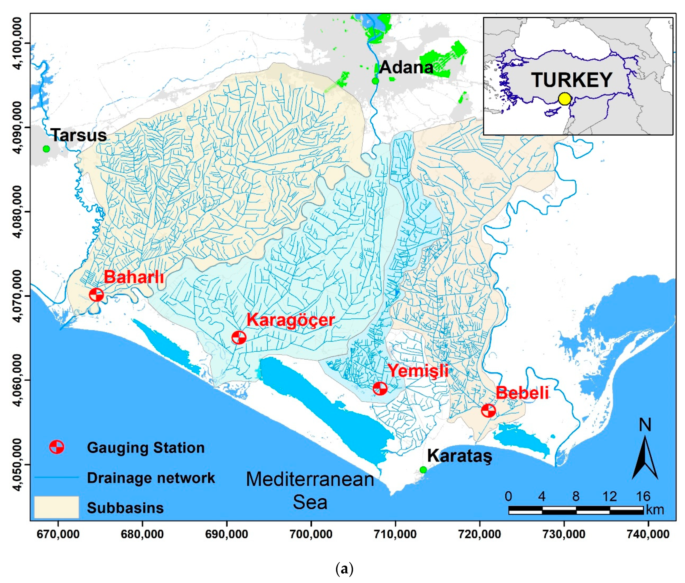
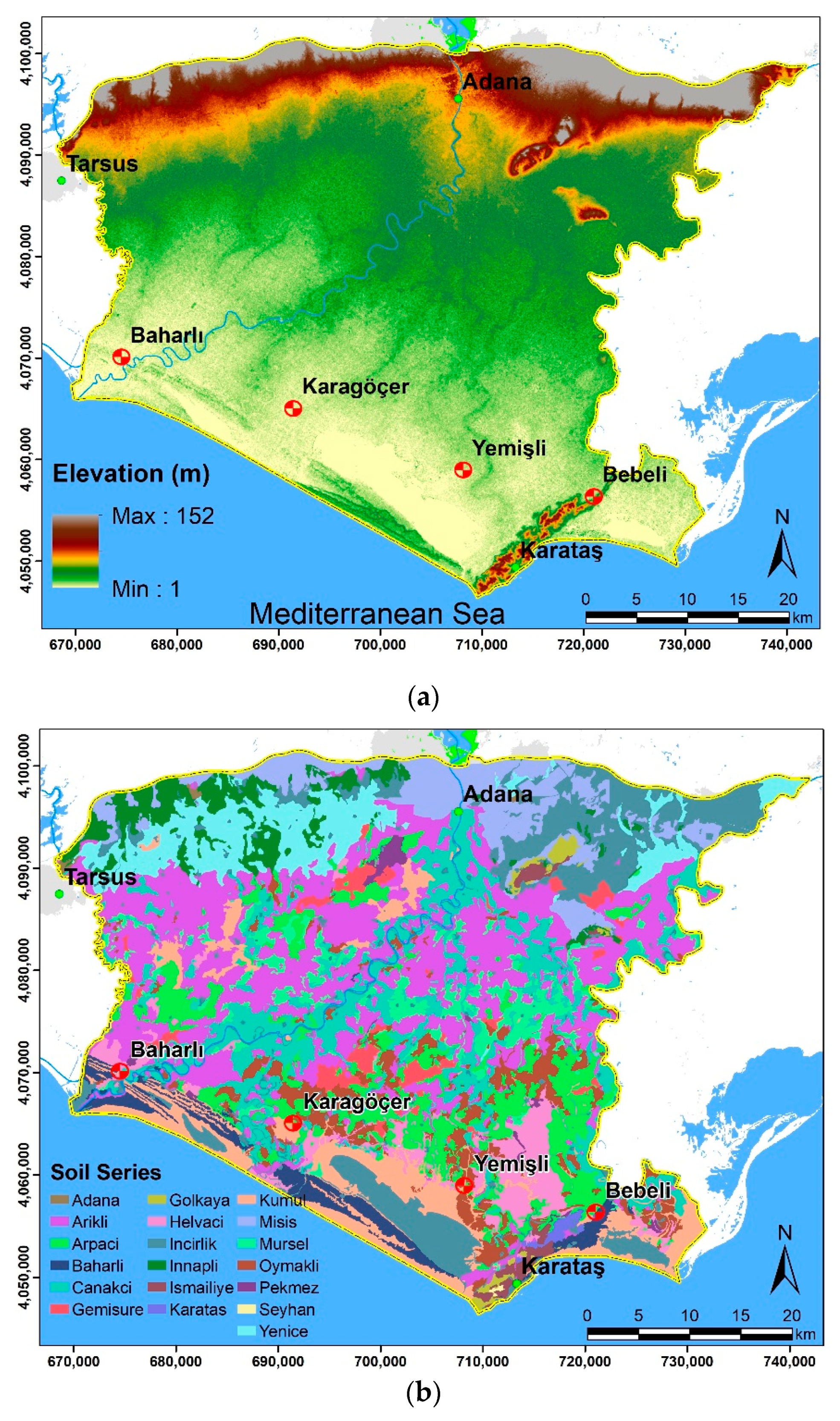
2.1. Study Area
2.2. Model Description
2.2.1. Model Inputs
2.2.2. Data Adjustments, Model Parametrization, and Setup
Ancillary Data
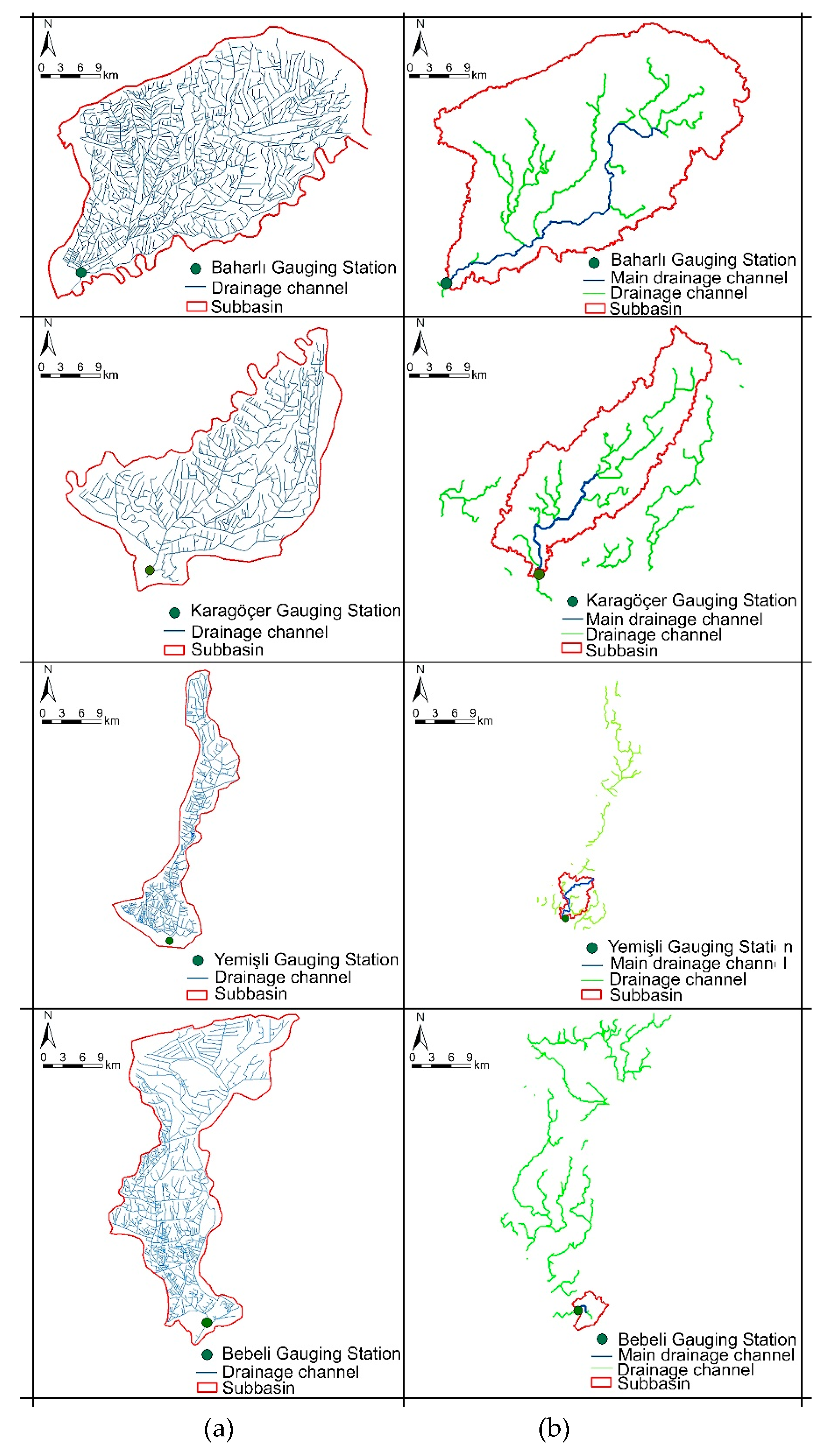
Drainage Networks
Sub-Basin Delineation
Hydrological Response Units
Time Series and Management Data
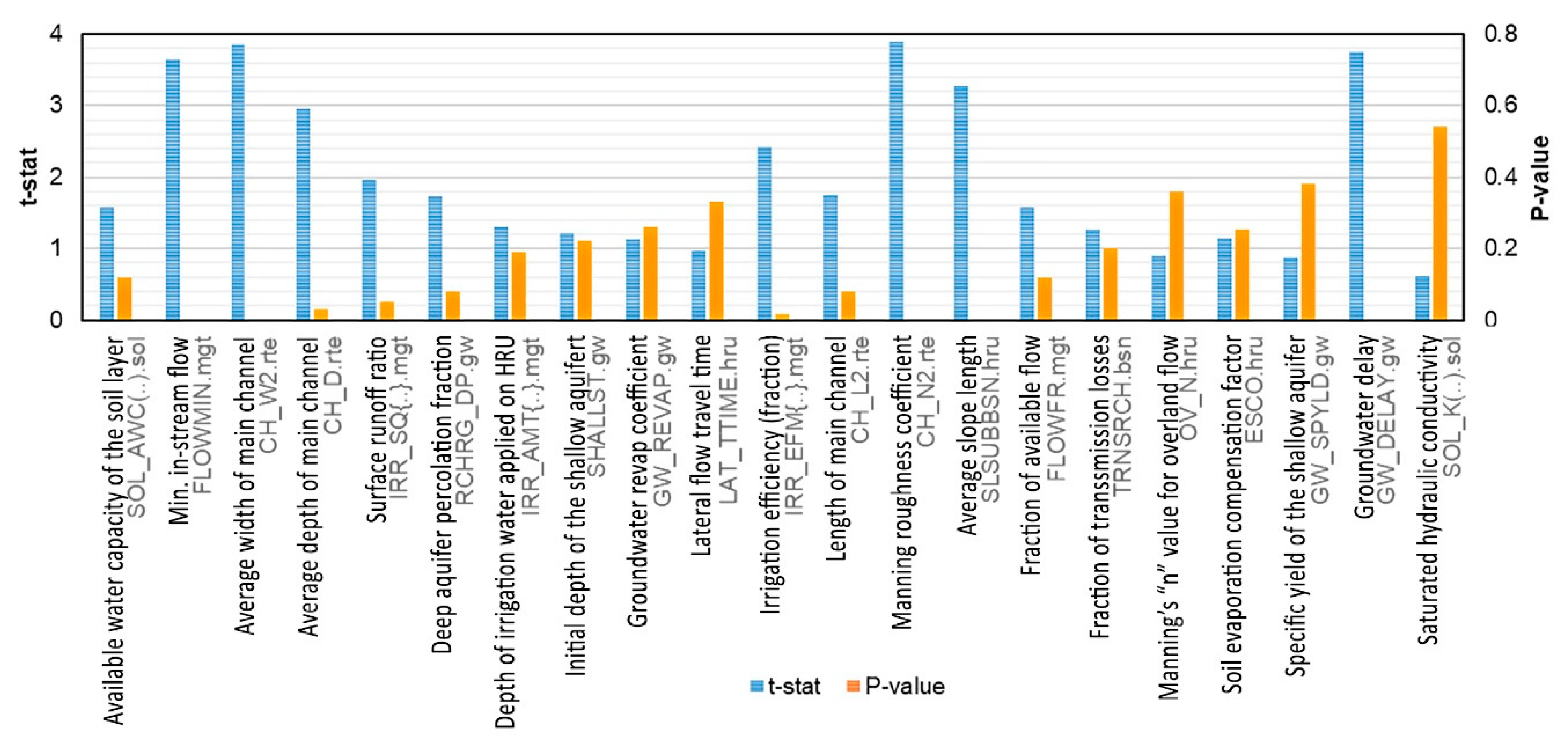
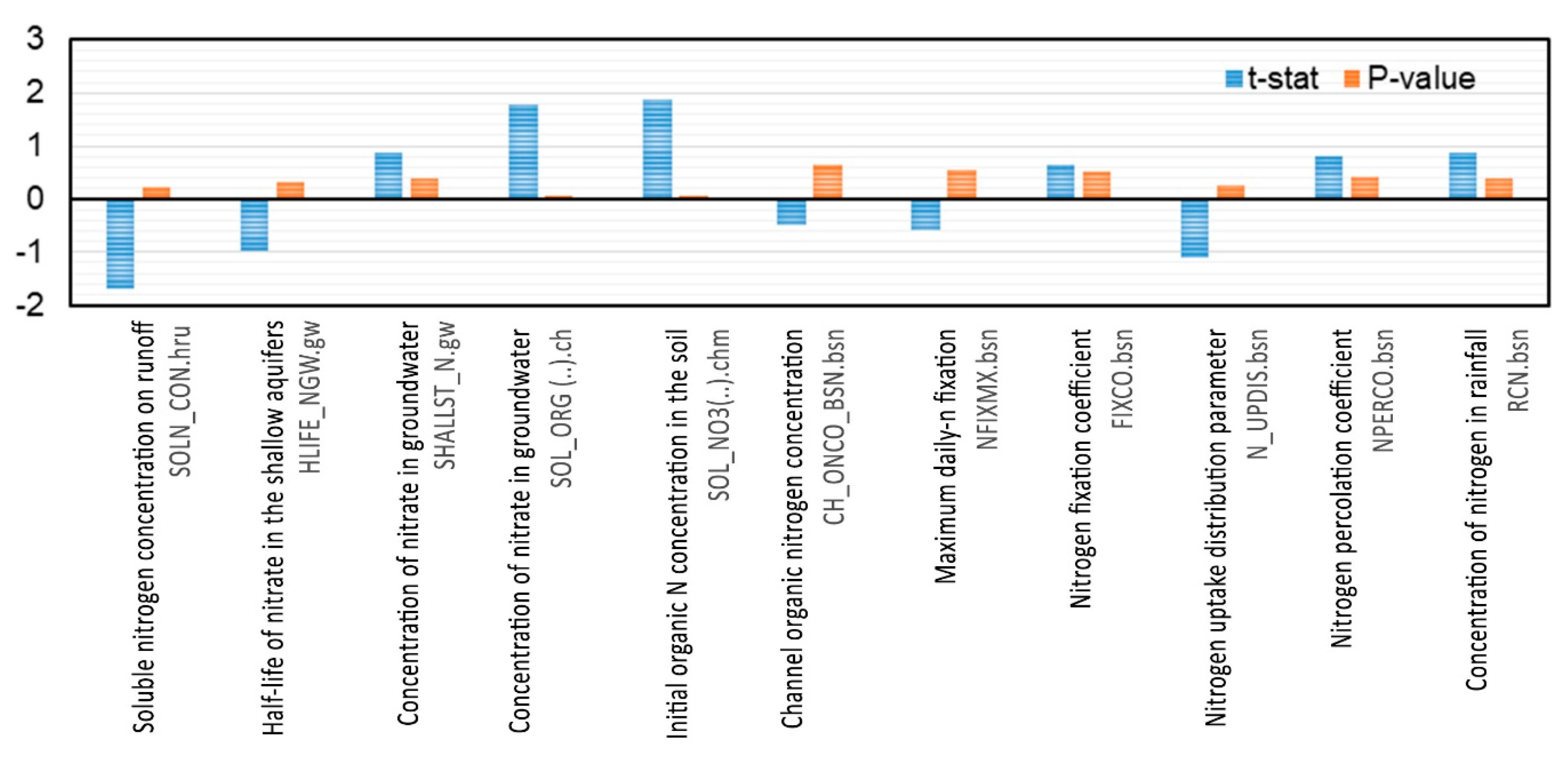
2.2.3. Model Calibration and Sensitivity Analysis
3. Results
3.1. Model Runs Using Default Parameter Conditions
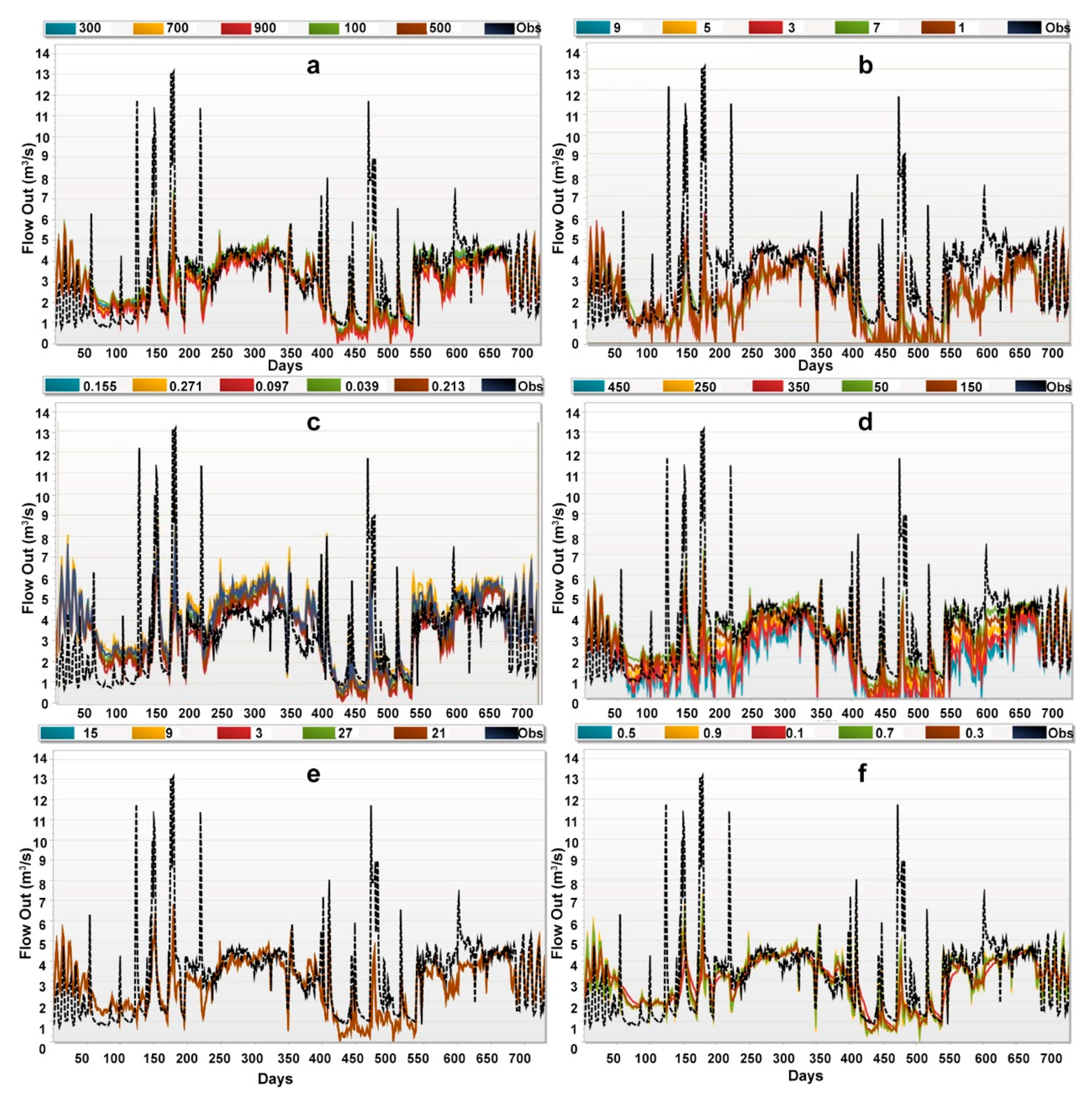
3.1.1. Model Calibration
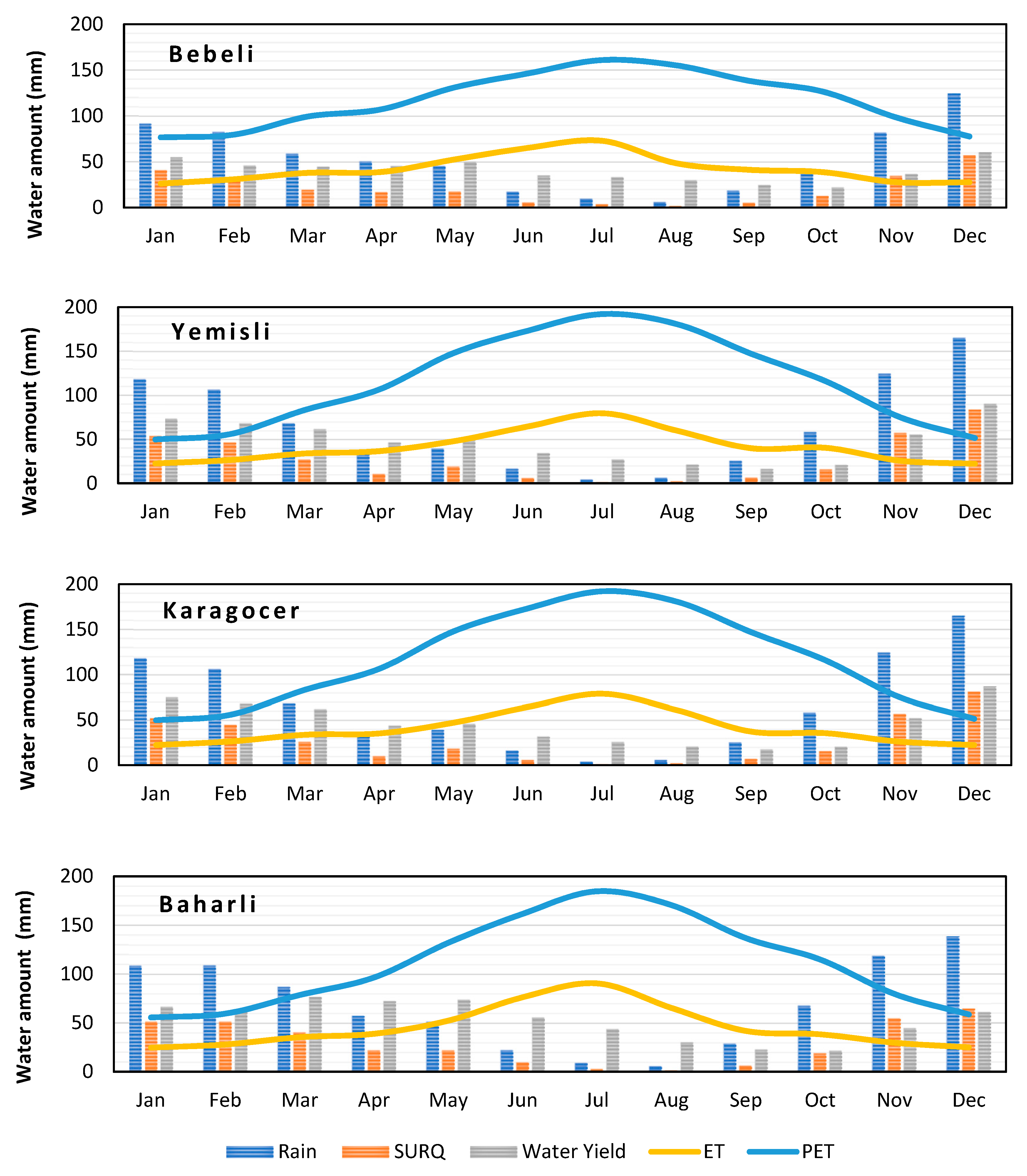
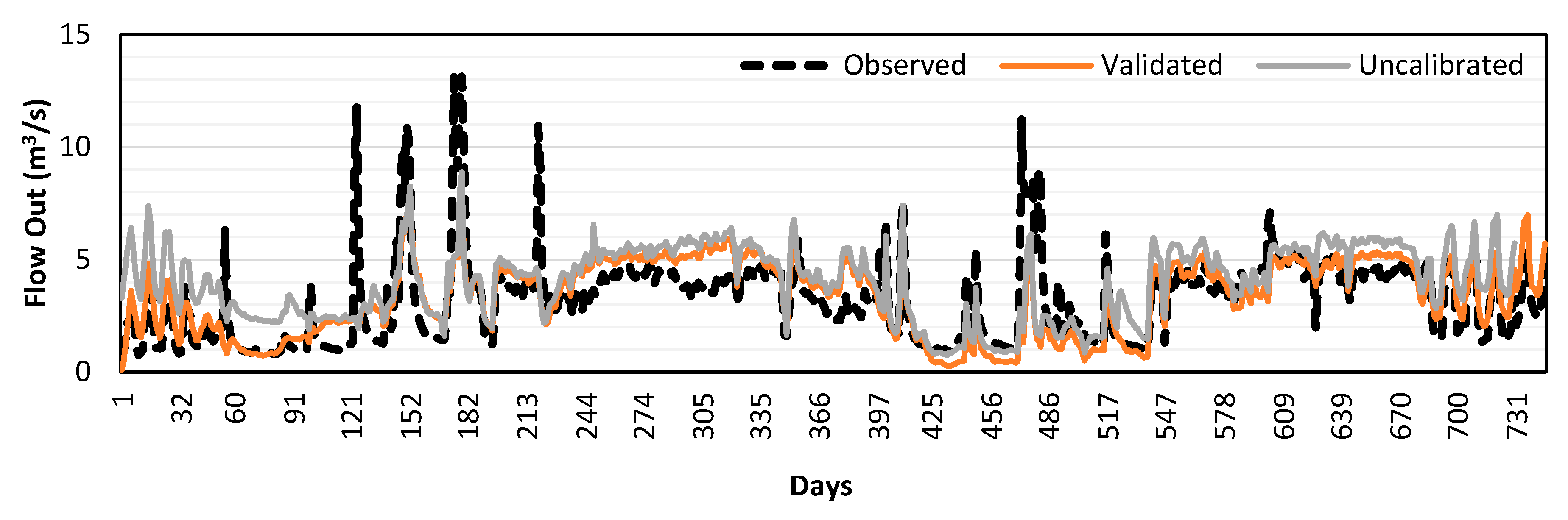
Water
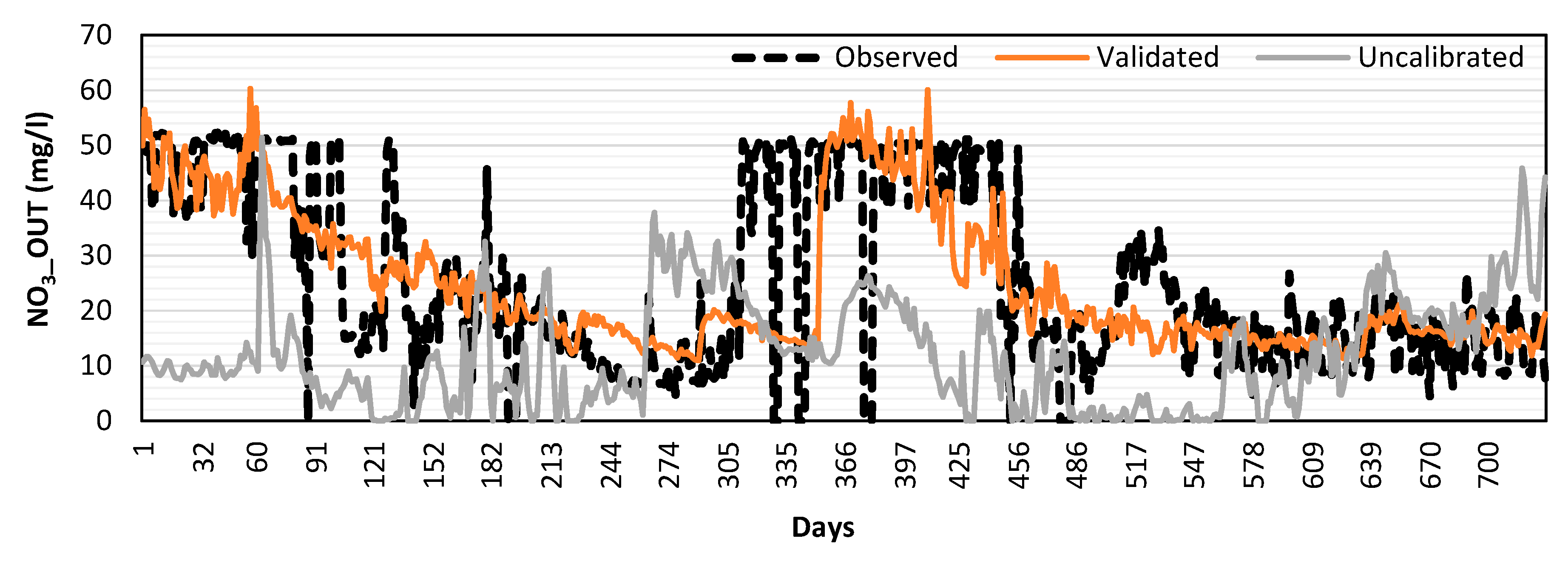
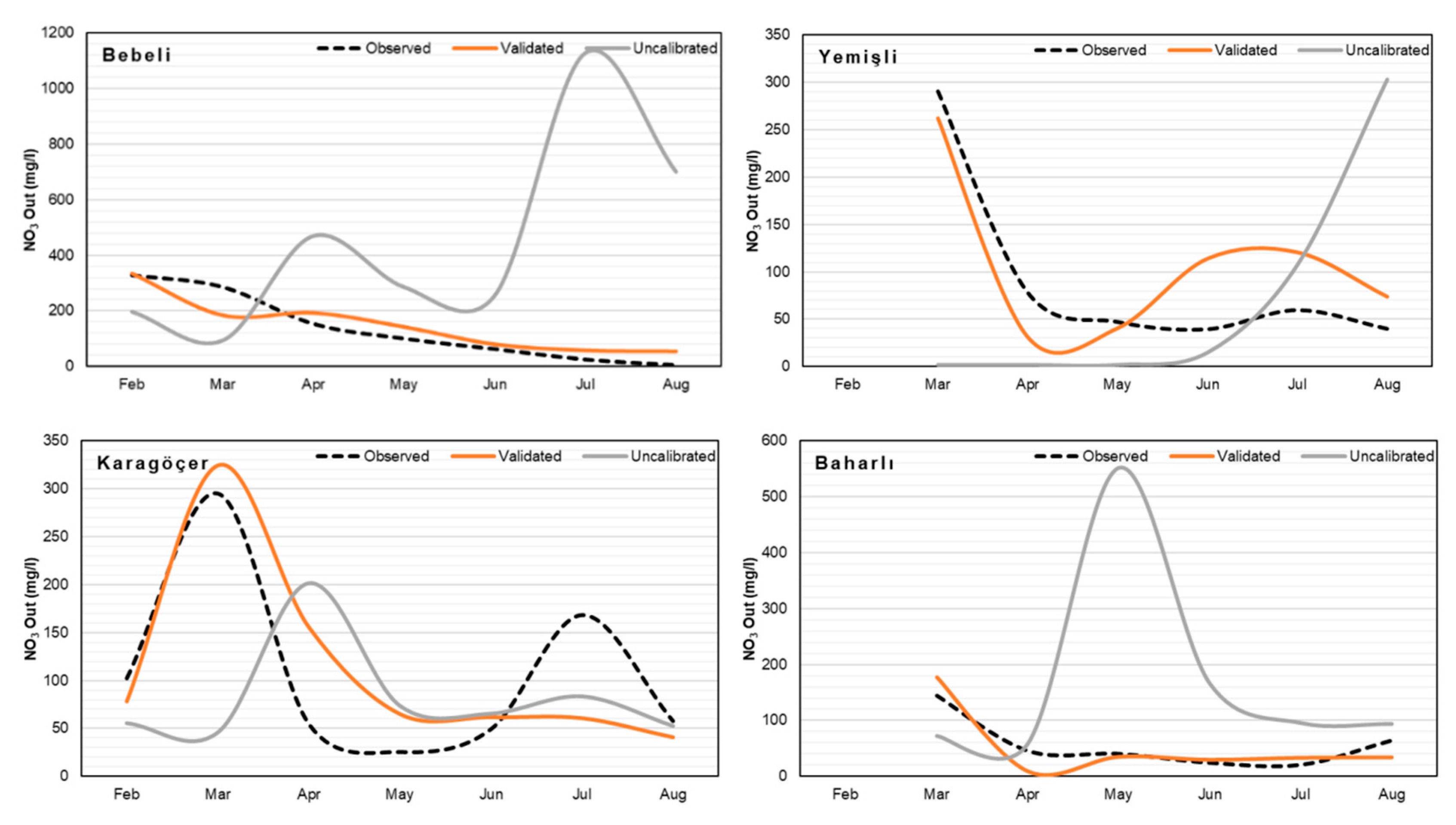
Nutrients
4. Discussion and Conclusions
Author Contributions
Funding
Conflicts of Interest
References
- Amatya, D.M.; Jha, M.K. Evaluating the SWAT model for a low-gradient forested watershed in coastal South Carolina. Trans. ASABE 2011, 54, 2151–2163. [Google Scholar] [CrossRef] [Green Version]
- Tripathi, M.P.; Raghuwanshi, N.S.; Rao, G.P. Effect of watershed subdivision on simulation of water balance components. Hydrol. Process. 2006, 20, 1137–1156. [Google Scholar] [CrossRef]
- Garbrecht, J.; Ogden, F.L.; DeBarry, P.A.; Maidment, D.R. GIS and distributed watershed models. I: Data coverages and sources. J. Hydrol. Eng. 2001, 6, 506–514. [Google Scholar] [CrossRef]
- Vogt, J.; Soille, P.; Colombo, R.; Paracchini, M.L.; de Jager, A. Development of a pan-European river and catchment database. Lect. Notes Geoinf. Cartogr. 2007, 121–144. [Google Scholar] [CrossRef]
- Reil, A.; Skoulikaris, C.; Alexandridis, T.K.; Roub, R. Evaluation of riverbed representation methods for one-dimensional flood hydraulics model. J. Flood Risk Manag. 2018. [Google Scholar] [CrossRef]
- Maidment, D.R. Arc Hydro: GIS for Water Resources; Environmental Systems Research Institute Inc.: Redlands, CA, USA, 2002; ISBN 1589480341. [Google Scholar]
- Arnold, J.G.; Srinivasan, R.; Muttiah, R.S.; Williams, J.R. Large area hydrologic modeling and assessment part I: Model development. J. Am. Water Resour. Assoc. 1998, 34, 73–89. [Google Scholar] [CrossRef]
- Schmalz, B.; Tavares, F.; Fohrer, N. Modelling hydrological processess in mesoscale lowland river basins with SWAT-Capabilities and challenges. Hydrol. Sci. J. 2008, 53, 989–1000. [Google Scholar] [CrossRef]
- Habeck, A.; Krysanova, V.; Hattermann, F. Integrated analysis of water quality in a mesoscale lowland basin. Adv. Geosci. 2005, 5, 13–17. [Google Scholar] [CrossRef] [Green Version]
- Krysanova, V.; Müller-Wohlfeil, D.I.; Becker, A. Development and test of a spatially distributed hydrological/water quality model for mesoscale watersheds. Ecol. Modell. 1998, 106, 261–289. [Google Scholar] [CrossRef]
- Krysanova, V.; Meiner, A.; Roosaare, J.; Vasilyev, A. Simulation modelling of the coastal waters pollution from agricultural watershed. Ecol. Modell. 1989, 49, 7–29. [Google Scholar] [CrossRef]
- Stefanova, A.; Hesse, C.; Krysanova, V.; Volk, M. Assessment of Socio-Economic and Climate Change Impacts on Water Resources in Four European Lagoon Catchments. Environ. Manag. 2019, 64, 701–720. [Google Scholar] [CrossRef] [Green Version]
- Arabi, M.; Govindaraju, R.S.; Hantush, M.M.; Engel, B.A. Role of watershed subdivision on modeling the effectiveness of best management practices with SWAT. J. Am. Water Resour. Assoc. 2006, 42, 513–528. [Google Scholar] [CrossRef]
- Al-Khafaji, M.S.; Al-Sweiti, F.H. Integrated Impact of Digital Elevation Model and Land Cover Resolutions on Simulated Runoff by SWAT Model. Hydrol. Earth Syst. Sci. Discuss. 2017, 1–26. [Google Scholar] [CrossRef] [Green Version]
- Lindsay, J.B. The practice of DEM stream burning revisited. Earth Surf. Process. Landf. 2016, 41, 658–668. [Google Scholar] [CrossRef]
- Amatya, D.M.; Radecki-pawlik, A. Flow Dynamics of Three Experiemental Forested Watersheds in coastal SC. Acta Sci. Pol. Form. Circumiectus 2007, 6, 3–17. [Google Scholar]
- Bárdossy, A. Calibration of hydrological model parameters for ungauged catchments. Hydrol. Earth Syst. Sci. 2007, 11, 703–710. [Google Scholar] [CrossRef] [Green Version]
- Blöschl, G. Rainfall-Runoff Modeling of Ungauged Catchments. In Encyclopedia of Hydrological Sciences; John Wiley & Sons, Ltd.: Chichester, UK, 2005. [Google Scholar]
- Nepal, S.; Flügel, W.A.; Krause, P.; Fink, M.; Fischer, C. Assessment of spatial transferability of process-based hydrological model parameters in two neighbouring catchments in the Himalayan Region. Hydrol. Process. 2017, 31, 2812–2826. [Google Scholar] [CrossRef]
- Donmez, C.; Berberoglu, S. A comparative assessment of catchment runoff generation and forest productivity in a semi-arid environment. Int. J. Digit. Earth 2016, 9, 942–962. [Google Scholar] [CrossRef]
- Cilek, A.; Berberoglu, S. Biotope conservation in a Mediterranean agricultural land by incorporating crop modelling. Ecol. Modell. 2019, 392, 52–66. [Google Scholar] [CrossRef]
- Sari, O. Modelling Hydrologic Dynamics of Lower Seyhan Basin by the Swat Model. Master’s Thesis, Department of Remote Sensing and Geographical Information Systems, Institute of Natural and Applied Sciences, Cukurova University, Adana, Turkey, 2018. [Google Scholar]
- Berberoglu, S.; Polat, S.; Ibrikci, H.; Donmez, C.; Satir, O.; Akin Tanriover, A.; Gultekin, U.; Kapur, B.; Erdogan, M.; Erdogan, N.; et al. Spatial Information Technology based Decision Support System for Seyhan Basin; Turkish Scientific and Research Council (TUBITAK) Project (ID:115Y063); Turkish Scientific and Research Council (TUBITAK): Adana, Turkey, 2019. [Google Scholar]
- Watanabe, T.; Nagano, T.; Kanber, R.; Kapur, S. An Integrated Approach to Climate Change Impact Assessment on Basin Hydrology and Agriculture. In Climate Change Impacts on Basin Agro-Ecosystems; Watanabe, T., Kapur, S., Aydın, M., Kanber, R., Akça, E., Eds.; Springer International Publishing: Cham, Switzerland, 2019; pp. 1–15. ISBN 978-3-030-01036-2. [Google Scholar]
- Guse, B.; Pfannerstill, M.; Strauch, M.; Reusser, D.E.; Lüdtke, S.; Volk, M.; Gupta, H.; Fohrer, N. On characterizing the temporal dominance patterns of model parameters and processes. Hydrol. Process. 2016, 30, 2255–2270. [Google Scholar] [CrossRef]
- Rahman, K.; Maringanti, C.; Beniston, M.; Widmer, F.; Abbaspour, K.; Lehmann, A. Streamflow Modeling in a Highly Managed Mountainous Glacier Watershed Using SWAT: The Upper Rhone River Watershed Case in Switzerland. Water Resour. Manag. 2013, 27, 323–339. [Google Scholar] [CrossRef] [Green Version]
- Zhou, P.; Huang, J.; Pontius, R.G.; Hong, H. New insight into the correlations between land use and water quality in a coastal watershed of China: Does point source pollution weaken it? Sci. Total Environ. 2016, 543, 591–600. [Google Scholar] [CrossRef] [PubMed]
- Strauch, M.; Bernhofer, C.; Koide, S.; Volk, M.; Lorz, C.; Makeschin, F. Using precipitation data ensemble for uncertainty analysis in SWAT streamflow simulation. J. Hydrol. 2012, 414, 413–424. [Google Scholar] [CrossRef]
- USDA Soil Conservation Service. Soil Conservation Service Engineering Division Section 4: Hydrology. In National Engineering Handbook; USDA Soil Conservation Service: Washington, DC, USA,, 1972. [Google Scholar]
- Vaché, K.B.; Eilers, J.M.; Santelmann, M.V. Water quality modeling of alternative agricultural scenarios in the U.S. Corn Belt. J. Am. Water Resour. Assoc. 2002, 38, 773–787. [Google Scholar] [CrossRef]
- Chaplot, V.; Saleh, A.; Jaynes, D.B.; Arnold, J. Predicting water, sediment and NO 3-N loads under scenarios of land-use and management practices in a flat watershed. Water. Air. Soil Pollut. 2004, 154, 271–293. [Google Scholar] [CrossRef]
- Behera, S.; Panda, R.K. Evaluation of management alternatives for an agricultural watershed in a sub-humid subtropical region using a physical process based model. Agric. Ecosyst. Environ. 2006, 113, 62–72. [Google Scholar] [CrossRef]
- Gassman, P.W.; Reyes, M.R.; Green, C.H.; Arnold, J.G. The soil and water assessment tool: Historical development, applications, and future research directions. Trans. ASABE 2007, 50, 1211–1250. [Google Scholar] [CrossRef] [Green Version]
- Akgul, M.A. Modelling Water and Nitrate Budget in Left Bank Irrigation of Lower Seyhan Plain. Master’s Thesis, Department of Remote Sensing and Geographical Information Systems, Institute of Natural and Applied Sciences, Cukurova University, Adana, Turkey, 2015. [Google Scholar]
- Abbaspour, K.C.; Vejdani, M.; Haghighat, S. SWAT-CUP calibration and uncertainty programs for SWAT. In Proceedings of the MODSIM07-Land, Water and Environmental Management: Integrated Systems for Sustainability, Christchurch, New Zealand, 10–13 December 2007; pp. 1596–1602. [Google Scholar]
- Setegn, S.G.; Srinivasan, R.; Melesse, A.M.; Dargahi, B. SWAT model application and prediction uncertainty analysis in the Lake Tana Basin, Ethiopia. Hydrol. Process. 2010, 24, 357–367. [Google Scholar] [CrossRef]
- Moriasi, D.N.; Arnold, J.G.; Van Liew, M.W.; Bingner, R.L.; Harmel, R.D.; Veith, T.L. Model Evaluation Guidelines for Systematic Quantification of Accuracy in Watershed Simulations. Trans. ASABE 2007, 50, 885–900. [Google Scholar] [CrossRef]
- Cakir, R.; Raimonet, M.; Sauvage, S.; Paredes-Arquiola, J.; Grusson, Y.; Roset, L.; Meaurio, M.; Navarro, E.; Sevilla-Callejo, M.; Lechuga-Crespo, J.L.; et al. Hydrological alteration index as an indicator of the calibration complexity ofwater quantity and quality modeling in the context of global change. Water 2020, 12, 115. [Google Scholar] [CrossRef] [Green Version]
- Nagelkerke, N.J.D. A note on a general definition of the coefficient of determination. Biometrika 1991, 78, 691–692. [Google Scholar] [CrossRef]
- Gupta, H.V.; Sorooshian, S.; Yapo, P.O. Status of Automatic Calibration for Hydrologic Models: Comparison with Multilevel Expert Calibration. J. Hydrol. Eng. 1999. [Google Scholar] [CrossRef]
- Tedeschi, L.O. Assessment of the adequacy of mathematical models. Agric. Syst. 2006, 89, 225–247. [Google Scholar] [CrossRef]
- Kapur, B.; Aydın, M.; Yano, T.; Koç, M.; Barutçular, C. Interactive Effects of Elevated CO2 and Climate Change on Wheat Production in the Mediterranean Region. In Climate Change Impacts on Basin Agro-Ecosystems; Watanabe, T., Kapur, S., Aydın, M., Kanber, R., Akça, E., Eds.; Springer International Publishing: Cham, Switzerland, 2019; pp. 245–268. ISBN 978-3-030-01036-2. [Google Scholar]
- Ben-Asher, J.; Yano, T.; Aydın, M.; Garcia y Garcia, A. Enhanced Growth Rate and Reduced Water Demand of Crop Due to Climate Change in the Eastern Mediterranean Region. In Climate Change Impacts on Basin Agro-Ecosystems; Watanabe, T., Kapur, S., Aydın, M., Kanber, R., Akça, E., Eds.; Springer International Publishing: Cham, Switzerland, 2019; pp. 269–293. ISBN 978-3-030-01036-2. [Google Scholar]
- Berberoğlu, S.; Evrendilek, F.; Dönmez, C.; Çilek, A. Estimating Spatio-temporal Responses of Net Primary Productivity to Climate Change Scenarios in the Seyhan Watershed by Integrating Biogeochemical Modelling and Remote Sensing. In Climate Change Impacts on Basin Agro-Ecosystems; Springer: Berlin/Heidelberg, Germany, 2019; pp. 183–199. [Google Scholar]
- Tanaka, K.; Fujihara, Y.; Topaloğlu, F.; Simonovic, S.P.; Kojiri, T. Impacts of Climate Change on Basin Hydrology and the Availability of Water Resources. In Climate Change Impacts on Basin Agro-Ecosystems; Watanabe, T., Kapur, S., Aydın, M., Kanber, R., Akça, E., Eds.; Springer International Publishing: Cham, Switzerland, 2019; pp. 71–97. ISBN 978-3-030-01036-2. [Google Scholar]
- Hoshikawa, K.; Nagano, T.; Kume, T.; Watanabe, T. Evaluation of Impact of Climate Changes in the Lower Seyhan Irrigation Project Area, Turkey. In Climate Change Impacts on Basin Agro-Ecosystems; Watanabe, T., Kapur, S., Aydın, M., Kanber, R., Akça, E., Eds.; Springer International Publishing: Cham, Switzerland, 2019; pp. 99–123. ISBN 978-3-030-01036-2. [Google Scholar]


| Data | Data Type | Source | Scale/Resolution | Data Description/Properties |
|---|---|---|---|---|
| Spatial Data | DEM | ASTER GDEM | 15 m | Stream network, sub-basin delineation, slope derivation |
| Satellite images | LANDSAT 7 ETM+ | 30 m | LULC, cultivated parcels | |
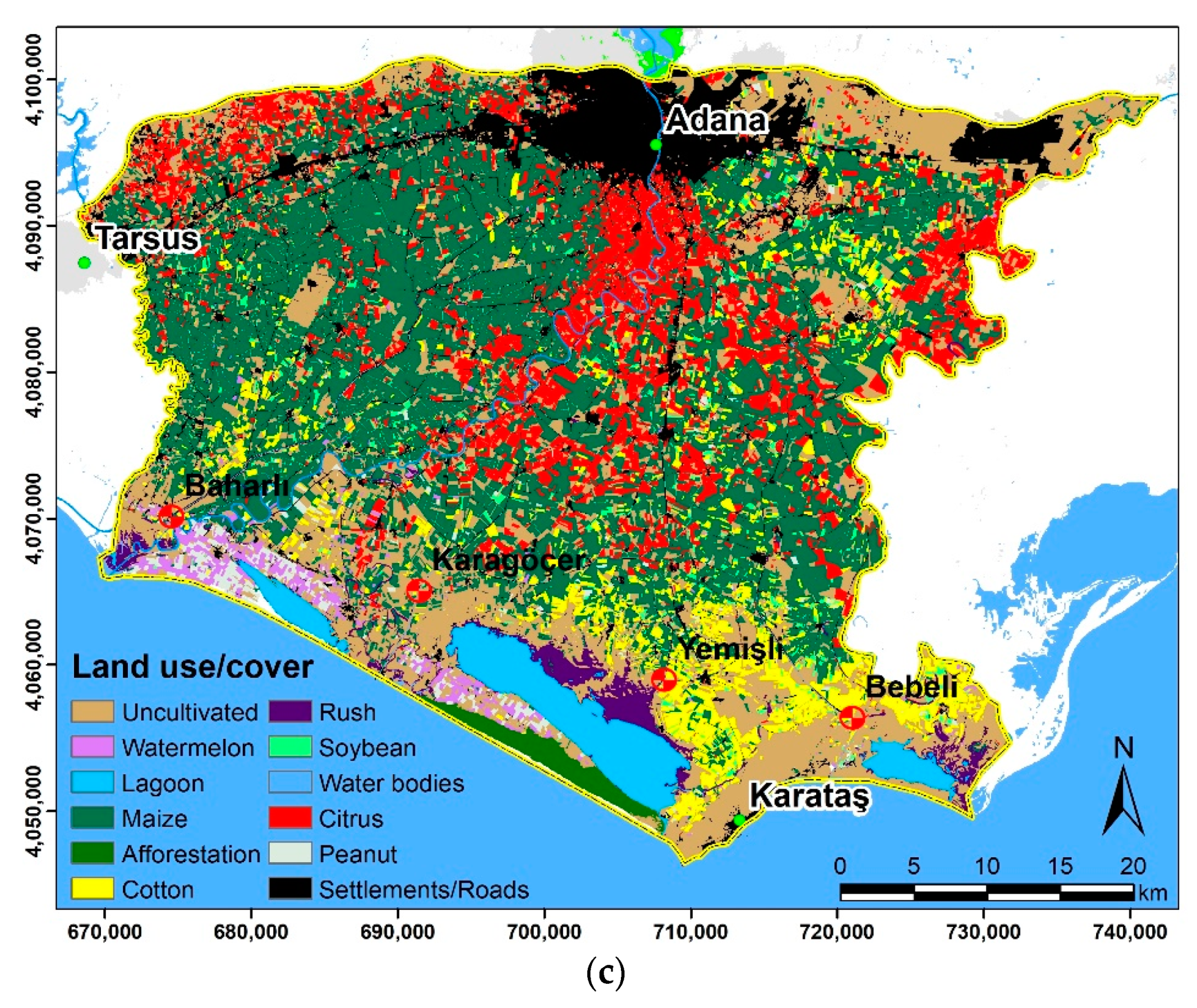
| LULC | Classified from LANDSAT 7 ETM+ | 30 m | 15 land cover/use classes. 95% (Kappa statistic) | |
| Soil | Derived from TUBITAK Project (No: 115Y063) | 1/250.000 | 17 soil series Soil physical properties including depth, saturated hydraulic conductivity, texture | |
| Stream networks | Digitized using stream burning method | 30 m | Including main drainage channels | |
| Hydrological Response Unit (HRU) | Derived using QGIS | 30 m | Comprising spatial information on heterogeneous units | |
| Hydro-meteorological Time-series | Temperature | Turkish State Meteorological Service | 13 stations | Daily climate data (2011–2018) |
| Relative humidity | ||||
| Wind speed | ||||
| Precipitation | ||||
| Solar radiation | ||||
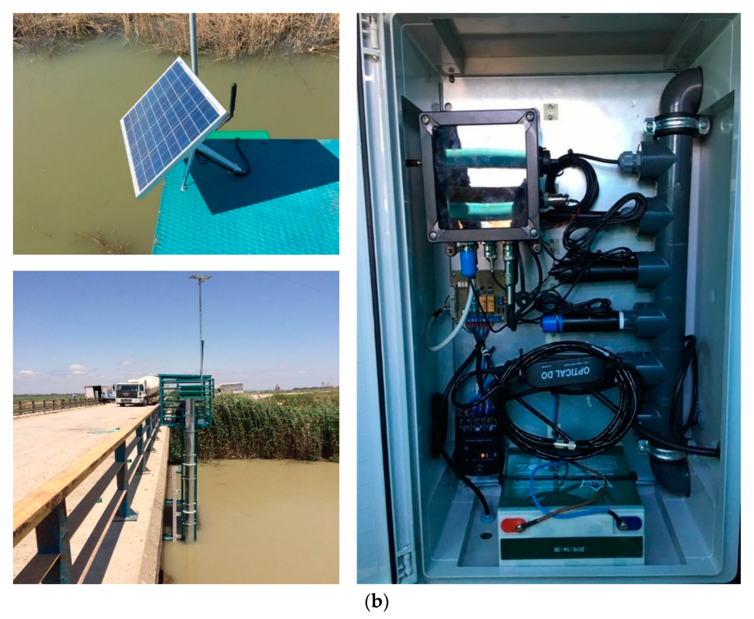
| Observed flow | Real-time stream gauging stations by TUBITAK Project (No: 115Y063) | Four gauging stations | Flow rates were calculated using this 15 min flow rates (ft3 s−1) to Derive mean daily outflow rates (m3 s−1) and daily total (mm) for each sub-basin (Sari, 2018). | |
| NO3 records | Real-time stream gauging stations by TUBITAK Project (No: 115Y063) | Four gauging stations | ||
| Land Management Information | Management/Point sources | Water use associations, expert opinion, and field campaigns | Planting, harvest, irrigation applications, fertilizer/pesticide/tillage applications for each crop |
| Stress Types (Number of Days/Year) | Sub-Basins | |||
|---|---|---|---|---|
| Baharli | Karagocer | Yemisli | Bebeli | |
| Water Stress | 73.85 | 84.62 | 59.87 | 56.38 |
| Temperature Stress | 88.86 | 89.09 | 99.81 | 84.44 |
| Nitrogen Stress | 73.72 | 40.66 | 67.15 | 50.89 |
| Phosphorus Stress | 14.33 | 8.45 | 6.27 | 8.87 |
| Hydrological Variables (mm) | Sub-Basins | |||
|---|---|---|---|---|
| Baharli | Karagocer | Yemisli | Bebeli | |
| Precipitation | 802.8 | 766.3 | 766.3 | 628.2 |
| Surface Runoff | 374.84 | 377.81 | 339.6 | 244.31 |
| Shallow Aquifer | 57.68 | 64.01 | 163.68 | NAN |
| Deep Aquifer Recharge | 4.23 | 4.57 | 9.92 | 2.12 |
| Total Aquifer Recharge | 84.55 | 90.52 | 198.44 | 42.47 |
| Total Water Yield | 436.93 | 446.46 | 513.74 | 268.26 |
| Percolation Out of the Soil | 83.81 | 89.52 | 196.96 | 42.22 |
| Actual Evapotranspiration (ET) | 356.6 | 323.2 | 386.9 | 352.1 |
| Potential Evapotranspiration (PET) | 1334.4 | 1376.5 | 1380.1 | 1399.9 |
| Average Annual Basin Values, Nutrients (kg/ha) | Sub-Basins | |||
|---|---|---|---|---|
| Baharli | Karagocer | Yemisli | Bebeli | |
| Organic N | 9.881 | 1.604 | 1.145 | 1.404 |
| Organic P | 1.205 | 0.221 | 0.156 | 0.188 |
| NO3 yield (SQ) (to Stream in Surface Runoff) | 3.399 | 2.679 | 2.872 | 2.173 |
| NO3 yield (LAT) (to Stream in Lateral Flow) | 0.009 | 0.012 | 0.025 | 0.009 |
| Sol-P yield | 0.033 | 0 | 0.131 | 0.049 |
| NO3 leached | 76.846 | 70.083 | 99.665 | 66.547 |
| P uptake | NaN | 12.379 | 14.411 | 17.754 |
| N uptake | 47.895 | 38.251 | 48.681 | 57.843 |
| P-Fertilizer applied | 7.402 | 4.286 | 4.773 | 5.764 |
| N-Fertilizer applied | 259.672 | 226.447 | 262.881 | 226.179 |
| Denitrification | 27.688 | 14.863 | 15.926 | 18.676 |
| NO3 in rainfall | 0 | 0 | 0 | 0 |
| Initial NO3 in soil | 52.219 | 53.21 | 55.548 | 52.412 |
| Final NO3 in soil | 225.04 | 202.345 | 243.52 | 214.992 |
| Initial org N in soil | 8721.166 | 82.616 | 85.152 | 82.174 |
| Final org N in soil | 8130.764 | 135.558 | 193.541 | 149.786 |
| NO3 in fertilizers | 16.823 | 9.742 | 10.848 | 13.101 |
| P uptake in yield | 2.88 | 1.58 | 2.82 | 3.972 |
| N removed in yield | 19.638 | 12.615 | 22.263 | 31.812 |
| Ammonia volatilization | 102.663 | 111.7 | 117.634 | 99.893 |
| Ammonia nitrification | 140.351 | 105.306 | 134.719 | 113.005 |
| Parameters (Part-A) | Best Value | Minimum Range | Maximum Range | Description |
|---|---|---|---|---|
| Management (Mgt) | ||||
| IRR_ASO | 0.4234 | 0 | 1 | Irrigation/flow ratio |
| IRR_EFF | 0.2939 | 0 | 1 | Irrigation efficiency |
| IRR_AMT | 31.51 | 0 | 100 | Irrigation application depth |
| IRR_EFM | 0.201 | 0 | 1 | Irrigation productivity |
| AUTOWSTRS | 0.179 | 0 | 1 | Water stress factor of the plants |
| Direction (rte) | ||||
| CH_D | 16.891 | 0 | 30 | Average main channel depth |
| CH_N2 | 0.1134 | 0.01 | 0.3 | Manning roughness coefficient |
| CH_L2 | 50.281 | 0 | 500 | Average main channel length |
| CH_W2 | 60.798 | 0 | 1000 | Average main channel width |
| Groundwater (gwt) | ||||
| GWQMN | 1863 | 0 | 5000 | Water depth coefficient in a shallow aquifer |
| GW_SPYLD | 0.177 | 0 | 0.4 | Specific yield of a shallow aquifer |
| GW_DELAY | 15.654 | 0 | 500 | Groundwater delay |
| GWREVAP | 0.12 | 0.02 | 0.2 | Groundwater “Revap” coefficient |
| REVAPMN | 224.02 | 0 | 500 | Threshold in a shallow aquifer for “revap” level depth |
| SHALLST | 12344 | 0 | 50000 | Initial depth of the shallow aquifer |
| DEEPST | 21234.5 | 0 | 50000 | Initial depth of the deep aquifer |
| GWHT | 12.62 | 0 | 25 | Water table depth |
| ALPHA_BF | 0.92 | 0 | 1 | Groundwater alpha factor |
| RCHRG_DP | 0.877 | 0 | 1 | Deep aquifer percolation factor |
| Parameters (Part-B) | Best value | Minimum Range | Maximum Range | Description |
| Management (Mgt) | ||||
| TRSRCH | 0.544 | 0 | 1 | Quantity function of water passing through the main channel to the deep aquifer |
| SLSUBBSN | 89.116 | 10 | 150 | Average slope length |
| SURLAG | 13.725 | 0.05 | 24 | Surface flow delay |
| MSK_X | 0.2382 | 0 | 0.3 | Weight factor Affecting of storage of water entering the river |
| MSK_CO1 | 2.105 | 0 | 10 | Controlling coefficient of storage timing of the water in the river |
| MSK_CO2 | 4.39 | 0 | 10 | Controlling coefficient of storage timing of the water in the river |
| EPCO | 0.395 | 0 | 1 | Plant uptake factor |
| EVLAI. | 0.121 | 0 | 10 | Leaf area Index with no evaporation |
| Soil | ||||
| SOL_K | 272.43 | 0 | 2000 | Soil hydraulic conductivity coefficient |
| SOL_AWC | 0.143 | 0 | 1 | Existing soil water holding capacity |
| SOL_CBN | 8.378 | 0.05 | 10 | Amount of soil organic carbon |
| SOL_BD | 1.432 | 0.9 | 2.5 | Soil bulk density |
| HRU | ||||
| ESCO | 0.0337 | 0 | 1 | Soil evaporation factor |
| OV_N | 19.654 | 0.01 | 30 | Manning “n” value for surface flow |
| LAT_TTIME | 118.52 | 0 | 180 | Lateral flow movement time |
| Hydrological Variables (mm) | Sub-Basins | |||
|---|---|---|---|---|
| Baharli | Karagocer | Yemisli | Bebeli | |
| Precipitation | 802.8 | 766.3 | 766.3 | 628.2 |
| Flow generation | 374.84 | 377.81 | 339.6 | 244.31 |
| Contribution of the Subsurface Current to Streams | 0.05 | 0.08 | 0.21 | 0.06 |
| Contribution of the groundwater Current to Streams | 4.27 | 4.53 | 10.01 | 2.15 |
| Amount of water from the shallow aquifer to plant/soil profile | 25.26 | 25.52 | 26.96 | 20.81 |
| Shallow aquifer discharge | 57.68 | 64.01 | 163.68 | NAN |
| Deep aquifer discharge | 4.23 | 4.57 | 9.92 | 2.12 |
| Amount of water entering both aquifers | 84.55 | 90.52 | 198.44 | 42.47 |
| Water yield from HRUs to Streams | 436.93 | 446.46 | 513.74 | 268.26 |
| Infiltrated water to the soil profile | 83.81 | 89.52 | 196.96 | 42.22 |
| Actual Evapotranspiration (ET) | 356.6 | 323.2 | 386.9 | 352.1 |
| Potential Evapotranspiration (PET) | 1334.4 | 1376.5 | 1380.1 | 1399.9 |
| Parameters | Best Value | Minimum Range | Maximum Range | Description |
|---|---|---|---|---|
| Basin (Bsn) | ||||
| CH_ONCO_BSN | 81.1828 | 0 | 100 | Organic nitrogen in the channel |
| NFIXMX.bsn | 10.255 | 1 | 20 | Daily maximum nitrogen fixing |
| FIXCO.bsn | 0.263 | 0 | 1 | Nitrogen fixation coefficient |
| N_UPDIS.bsn | 28.238 | 0 | 100 | Nitrogen uptake and distribution parameters |
| NPERCO.bsn | 0.3938 | 0 | 1 | Nitrogen infiltration coefficient |
| RCN.bsn | 1.1891 | 0 | 15 | Nitrogen in the rain |
| Groundwater (gwt) | ||||
| SHALLST_N | 740.31 | 0 | 1000 | NO3 water in groundwater contribution to flow |
| HLIFE_NGW | 105.744 | 0 | 200 | Half-life of NO3 in a shallow aquifer |
| HRU | ||||
| SOLN_CON | 5.157 | 0 | 10 | Soluble nitrogen concentration after applying urban Best Management Practices (BMP) |
| Chemical (chm) | ||||
| SOL_NO3 | 28.93 | 0 | 100 | The initial concentration of NO3 in soil |
| SOL_ORGN | 11.24 | 0 | 100 | The initial amount of NO3 in soil |
| Sub-Basins | Flow | NO3 | ||||||||||
|---|---|---|---|---|---|---|---|---|---|---|---|---|
| Calibration (2011–2012) | Validation (2013–2018) | Calibration (2011–2012) | Validation (2013–2018) | |||||||||
| E | r2 | PBIAS | E | r2 | PBIAS | E | r2 | PBIAS | E | r2 | PBIAS | |
| Bebeli | 0.44 | 0.47 | −0.1 | 0.64 | 0.70 | +4.0 | 0.45 | 0.48 | −9.4 | 0.82 | 0.85 | +3.4 |
| Yemişli | 0.15 | 0.22 | −0.63 | 0.60 | 0.68 | +3.3 | −0.44 | 0.23 | −15.9 | 0.72 | 0.75 | +2.9 |
| Karagöçer | 0.01 | 0.08 | −2.9 | 0.57 | 0.66 | 0 | 0.10 | 0.18 | −4.8 | 0.53 | 0.61 | +3.8 |
| Baharlı | 0.13 | 0.44 | −0.1 | 0.63 | 0.82 | +4.1 | 0.21 | 0.43 | 0 | 0.66 | 0.85 | +7 |
Publisher’s Note: MDPI stays neutral with regard to jurisdictional claims in published maps and institutional affiliations. |
© 2020 by the authors. Licensee MDPI, Basel, Switzerland. This article is an open access article distributed under the terms and conditions of the Creative Commons Attribution (CC BY) license (http://creativecommons.org/licenses/by/4.0/).
Share and Cite
Donmez, C.; Sari, O.; Berberoglu, S.; Cilek, A.; Satir, O.; Volk, M. Improving the Applicability of the SWAT Model to Simulate Flow and Nitrate Dynamics in a Flat Data-Scarce Agricultural Region in the Mediterranean. Water 2020, 12, 3479. https://doi.org/10.3390/w12123479
Donmez C, Sari O, Berberoglu S, Cilek A, Satir O, Volk M. Improving the Applicability of the SWAT Model to Simulate Flow and Nitrate Dynamics in a Flat Data-Scarce Agricultural Region in the Mediterranean. Water. 2020; 12(12):3479. https://doi.org/10.3390/w12123479
Chicago/Turabian StyleDonmez, Cenk, Omer Sari, Suha Berberoglu, Ahmet Cilek, Onur Satir, and Martin Volk. 2020. "Improving the Applicability of the SWAT Model to Simulate Flow and Nitrate Dynamics in a Flat Data-Scarce Agricultural Region in the Mediterranean" Water 12, no. 12: 3479. https://doi.org/10.3390/w12123479