Soil Moisture Estimation Using Citizen Observatory Data, Microwave Satellite Imagery, and Environmental Covariates


University of Miskolc, Institute of Geography and Geoinformatics, 3515 Miskolc, Hungary
*
Author to whom correspondence should be addressed.
Water 2020, 12(8), 2160; https://doi.org/10.3390/w12082160
Submission received: 8 June 2020
/
Revised: 20 July 2020
/
Accepted: 24 July 2020
/
Published: 30 July 2020
(This article belongs to the Section Water, Agriculture and Aquaculture)
Abstract
:Soil moisture (SM) is a key variable in the climate system and a key parameter in earth surface processes. This study aimed to test the citizen observatory (CO) data to develop a method to estimate surface SM distribution using Sentinel-1B C-band Synthetic Aperture Radar (SAR) and Landsat 8 data; acquired between January 2019 and June 2019. An agricultural region of Tard in western Hungary was chosen as the study area. In situ soil moisture measurements in the uppermost 10 cm were carried out in 36 test fields simultaneously with SAR data acquisition. The effects of environmental covariates and the backscattering coefficient on SM were analyzed to perform SM estimation procedures. Three approaches were developed and compared for a continuous four-month period, using multiple regression analysis, regression-kriging and cokriging with the digital elevation model (DEM), and Sentinel-1B C-band and Landsat 8 images. CO data were evaluated over the landscape by expert knowledge and found to be representative of the major SM distribution processes but also presenting some indifferent short-range variability that was difficult to explain at this scale. The proposed models were evaluated using statistical metrics: The coefficient of determination (R2) and root mean square error (RMSE). Multiple linear regression provides more realistic spatial patterns over the landscape, even in a data-poor environment. Regression kriging was found to be a potential tool to refine the results, while ordinary cokriging was found to be less effective. The obtained results showed that CO data complemented with Sentinel-1B SAR, Landsat 8, and terrain data has the potential to estimate and map soil moisture content.
1. Introduction
Soil moisture (SM) is a key variable in the climate system and a key parameter in earth surface processes, particularly in water and energy cycles, as it impacts the total volume of water following on the earth’s surface and beneath the surface [1]. SM is defined as the volume of water content (units (vol/vol)) at a particular time within a particular space of the soil profile [2]. Several soil and landscape properties influence SM. Therefore, the correlation between different soil and landscape properties is critical in understanding the change in spatial and temporal soil moisture patterns.
Even though a large number of local and regional soil moisture networks are operating worldwide, they lack common standards (e.g., observed variables, sensor types, and sensor setup, etc.) and the generated data are often not freely available [3]. The International Soil Moisture Network (ISMN) is an international initiative trying to overcome such issues [4,5]. In situ soil moisture observations are collected from various networks distributed all over the globe, harmonized in terms of the sampling interval, units, and data format, and made freely available to the public through a web portal [6]. However, the number of observation sites and their density is very low. Therefore, it is evident that there is a great potential offered by COs (e.g., GROW Observatory) to contribute with an unprecedented stream of data from thousands of sensors.
Citizen science is rapidly developing in the 21st century, whereby data collection is conducted by or with non-experts [7]. Despite the long history of ‘citizen observatory’ (CO), quality assurance for the scientific use of citizen science-generated data is still missing [8]. Citizen science projects have been dominated by biodiversity topics [9], and weather and climate topics [10]. The GROW Observatory monitors soil properties, aiming to engage a target audience of smallholders, and community groups practicing sustainable growing [3].
The project aimed to demonstrate a complete ‘citizens’ observatory’ system for monitoring soil moisture, land use, and landcover; contributing in situ data for satellite validation; creating useful data products and applications; and finally giving a local context on the soil to local farmers [3,11]. Scientific studies to evaluate CO data interpretation and SM mapping on a large scale are needed to support agriculture, especially precision farming. This study aimed to contribute to this process with the development and testing of several digital soil mapping (DSM) procedures.
DSM [12,13] has allowed researchers to map soil properties quantitatively with the help of different data sources and on a range of different spatial scales [14,15]. DSM requires a smaller soil sampling effort, compared to more traditional mapping methods [14,16]. Once the smaller amount of sampled soil data is harmonized with environmental covariates from different sources, DSM can be a very powerful tool in the estimation of soil moisture and various soil properties [17]. The available SM measurements and monitoring sites are minimal and not very beneficial to local users. A potential way to fill this data gap is citizen observatory (CO). GROW Observatory collected a relatively large geo-referenced dataset of SM of the upper 10 cm, having the aim of producing observed data for Sentinel 1 applications [3].
To date, a large proportion of satellite imagery-based SM estimations focus on global and national scales [18,19]. Freely accessible satellite radar data, like Sentinel-1, have great potential in SM estimation [20], but reliable products require field data for calibration, which is one of the most limiting factors. Therefore, systems able to measure dynamic soil properties like SM are very rare, and are limited to a few observation sites and are mainly lacking the spatial interpolation procedures [21,22]. Despite the difficulties, the number of papers dealing with SM estimation using radar satellite data for irrigation and farming applications is increasing [23,24].
Zribi et al. [20], reviewed emerging SM estimation studies. Gharechelou et al. [25] ran several interpolation methods (inverse distance weighting, kriging, and co-kriging) to derive and evaluate SM maps for an arid area. The produced maps were compared to each other and validated using ground truth data. Keskin and Grunwald [26] used regression kriging (RK) for spatial interpolation of several soil properties. Han et al. [27] used MODIS data to estimate SM. Zeng et al. [28] performed cokriging using temporal backscatter ratios to estimate soil moisture on bare land using three variables, which were based on cross-semivariogram and cross-variance over 91 sampling points. The results showed a root mean square error (RMSE) value of between 2.669 and 2.701 over five months (December to April). Chatterjee et al. [29] tested two empirical models: A multiple linear regression model against the cubist model using in situ soil sensor SM measurements (used as the model response), Sentinel-1 data, and various ancillary data (USGS DEM, Sentinel 1, US National Land Cover Database, and the Probabilistic Remapping of Soil Survey Geographic (POLARIS) dataset). The statistical metric used to determine the model was R2. The Cubist model (0.56) performed better than the multiple linear regression (0.24) in land that had a specific crop type. The MLR results are similar to results obtained in our study and show that MLR at times cannot account for the complex relationship between soil moisture and satellite imagery. Zhang et al. [30] used three kriging methods (extended, ordinary, and cokriging) to interpolate near-surface soil moisture data measured by wireless sensor networks using the remote sensing-derived spectral variables, NDVI and albedo, in the interpolation algorithm. The visual results indicated that the result from extended kriging showed more spatial details than that of ordinary kriging or cokriging. However, the root mean square error (RMSE) of extended kriging (2.41) was found to be the smallest among the four (RMSE ranged from 2.62 to 3.01) interpolation results.
Bousbih et al. [23] used integrated Sentinel 1 and 2 datasets for field-scale SM estimation in a semi-arid region using an integrated decision tree estimation procedure. Two models were compared, a neural network classification and a direct water cloud model. They concluded that the approach is promising and the RMSE values ranged between 4.8 and 6.4. vol % and the R2 values ranged between 0.4 and 0.58. Xing et al. [24] used Radarsat-2 data for SM estimation and applied a modified water cloud model to remove the vegetation effect and applied the Dubois model to retrieve the dielectric constant and calculate the volumetric soil moisture. The final RMSE value was 4.43, with an R2 of 0.71.
Therefore, this research aimed to develop a method to estimate, test, and evaluate soil moisture spatially and temporally by integrating terrain and remote sensing data, like Sentinel-1 and Landsat-derived NDVI products. The study was carefully carried out through the following steps: (1) Establishment of an in situ soil moisture sampling design using low-cost soil sensors from the GROW example; (2) selection of environmental covariates that had the highest statistical correlation with soil moisture; (3) the creation and simulation of a quantitative approach for the estimation of soil moisture that is simple and data extensive—easy and free to access data; and (4) the conduction of a statistical analysis using multiple linear regression modelling, where regression kriging and cokriging were developed, analyzed, and compared [31]. Finally, the study examined if low-cost sensors are suitable devices in estimating soil moisture data across different geomorphological units to aid farming activities and scientific research.
2. Study Area
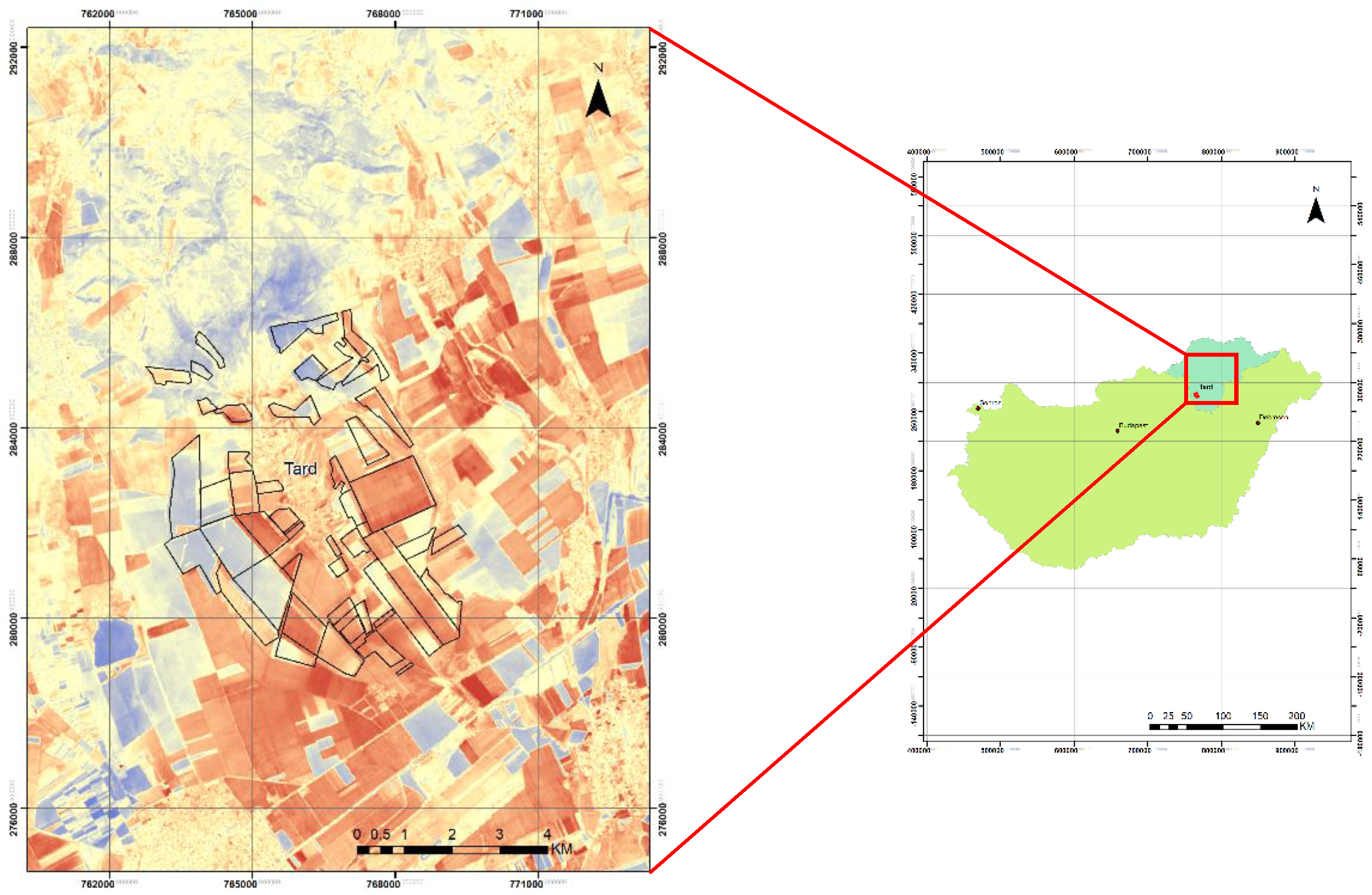
The study area comprised 1700 hectares (ha) of agricultural land. It is located on the southern tip of the mountain range of the North-Western Carpathians and the southern dissected foot slopes of the Bükk Mountains (Figure 1), near the village of Tard (47°52′33.67″ N, 20°35′56.53″ E). Geomorphologically, the area consists of two south-facing plateaus, which are split by the Tardi stream. The average elevation ranges between 150 and 200 m above mean sea level and a moderately warm-dry climate characterizes the region.
The latitude difference between the area is negligible from the macroclimate aspect; only the terrain factors influence the differences between the different microclimatic areas. The average annual temperature in the higher areas is 8 °C and in the lower areas is 9–10 °C. From mid-April to mid-October, the number of frost-free days is approximately 185 days, but the terrain greatly influences them. The average maximum summer temperature is 34 °C, and the mean winter minimum is −17 °C. The yearly amount of precipitation is approximately 640 mm while during the planting season period, it is measured to be approximately 340–380 mm. The average number of days of snow covering the surface is around 45 days, with an approximate thickness of 160–180 mm.
The crops planted during the study period were mainly winter wheat and sorghum. The latter one was secondary sowing, because rapeseed, which was planted in the fall, could not germinate due to extreme drought. The winter wheat was planted in early October and was harvested in July, so vegetation cover was permanent on the test fields with increasing biomass covering the surface. The height of the wheat was 10–20 cm in January and February and reached its full coverage in May with a height of approximately 60 cm with complete coverage of the soil surface. This temporal change of the covering biomass may have potentially decreased the model performance.
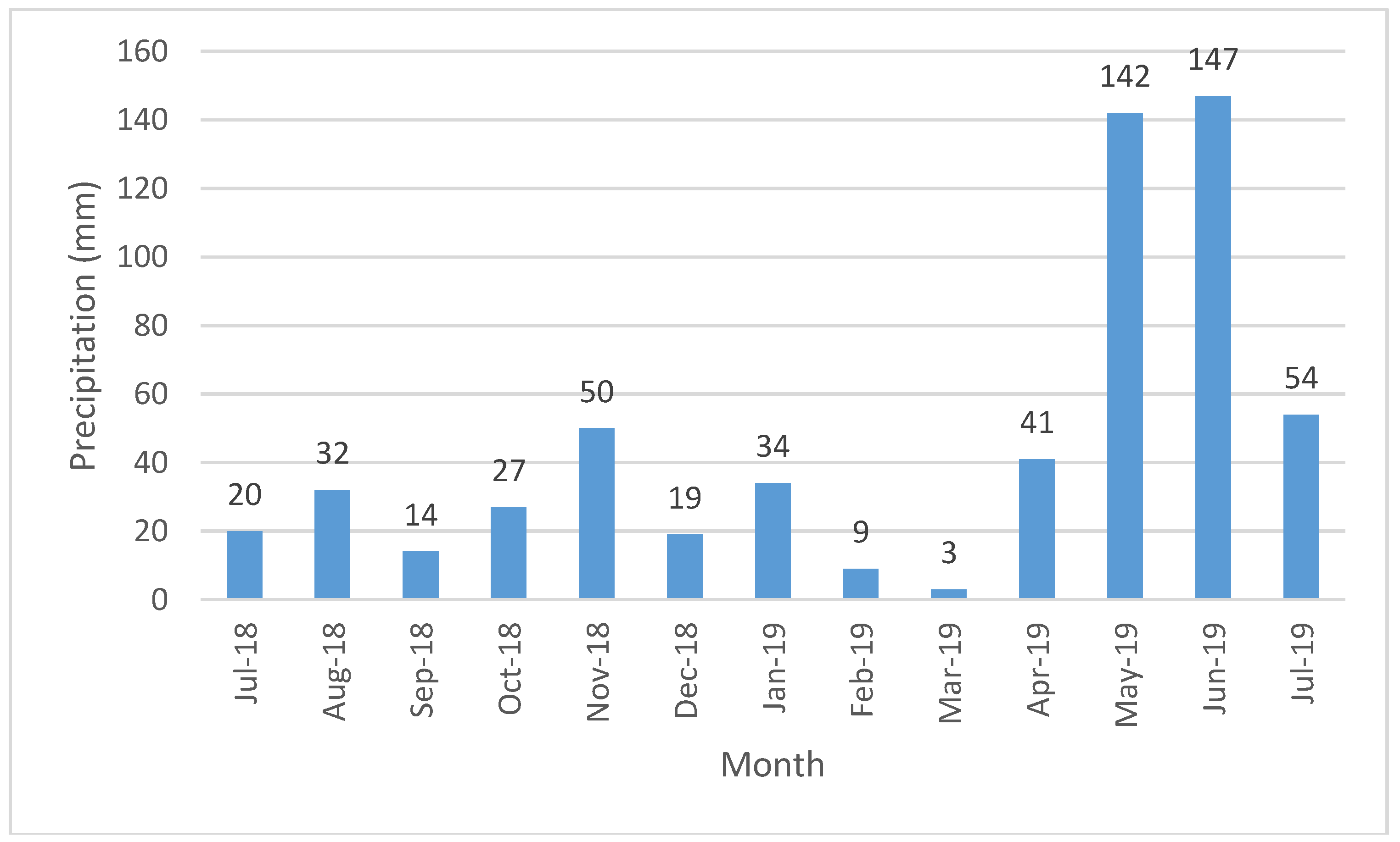
The weather in the study period varied a lot. The fall and winter were extremely dry, with some precipitation in November to January and no precipitation in February and March. There was a change from April to June, with extremely high precipitation (Figure 2) and a warming temperature that increased the evapotranspiration.
The soils of the region are mainly Mollic Vertisols [32] (Udic Haplustert [33]), which covers 80% of the region, namely the wide plateaus. The valley bottom has a loam texture and Gleyic Chernozems [32] (Cumulic Endoaquolls [33]) while the steep valley sides are a loamy sand texture Arenosols. The northern edge becomes a steep and sandy loam Luvisol [32] (Alfisol [33]) area with a lot of rhyolite tuff close to the surface; this is where the land use is changing from arable land to forest towards the mountain range.
3. Materials and Methods
3.1. Materials
3.1.1. Field Data
Soil moisture measurements were carried out using a low-cost sensor (Flower Power developed by Parrot S.A., Paris, France) at a depth of 0–10 cm below the surface of the ground. The low-cost sensors provide SM data in the upper 10 cm, soil temperature, light intensity, and conductivity. The reason for the selection of the upper 10 cm by the GROW project was to potentially provide validation data for Sentinel-1 images, which have a comparable penetration depth.
The measurements were logged every 15 min. The SM lines of drying—no precipitation with steady circumstances—showed clear trends with some daily fluctuation, which we regarded as artefacts due to the sudden temperature increase. These temperature values were used as input variables for the SM estimation and results in an erroneous estimation. In order to decrease its impact, soil moisture measurements were chosen at 2 a.m. of every selected day because, at this time, there was very little influence from any environmental factors, such as light, temperature, and evapotranspiration. Dates were chosen by the availability of Sentinel-1 data. NDVI was calculated from the closest cloud-free dates of the available satellite products, which happened to be Landsat 8 data. So, the Sentinel 1B and field data were from the same day, and the NDVI was 1 to 3 days after the selected dates, depending on the month. A systematic network was designed to capture the geomorphological and soil variation to develop an optimal setup, whereby the sensor performance was characterized. Sensors were placed in all representative geomorphological units of the study area to ensure the thematic coverage was filled.
The total area of the pilot site, where in situ soil moisture sensors were installed, was approximately 1200 ha of the total 1700 ha. This highlighted that more than 70% of the area was included, indicating a good variance in soil types and land use. In order to get an appropriate spatial distribution of sensors, the sensors were purposively placed at representative spots in all geomorphologic units. Catenas/toposequences were also defined to study the transition zones. The geomorphologic units were defined by the (soil and terrain digital database) e–SOTER methodology [34].
The total number of sensors placed in the study area ranged from 44 to 76 sensors depending on the month. Then, in each month, a total of 36 parcels were chosen for in situ soil moisture measurements. However, the major focus was placed on 12 of them having winter wheat, because it was the only crop that was consecutively in the field for the duration of the study. The influence of vegetation was more towards the end of the study period due to the growth of the wheat, which resulted in the backscatter coefficient having more noise. Fieldwork was conducted from January 2019 to June 2019 to understand the soil moisture change during different seasons.
3.1.2. Sentinel 1 Imagery
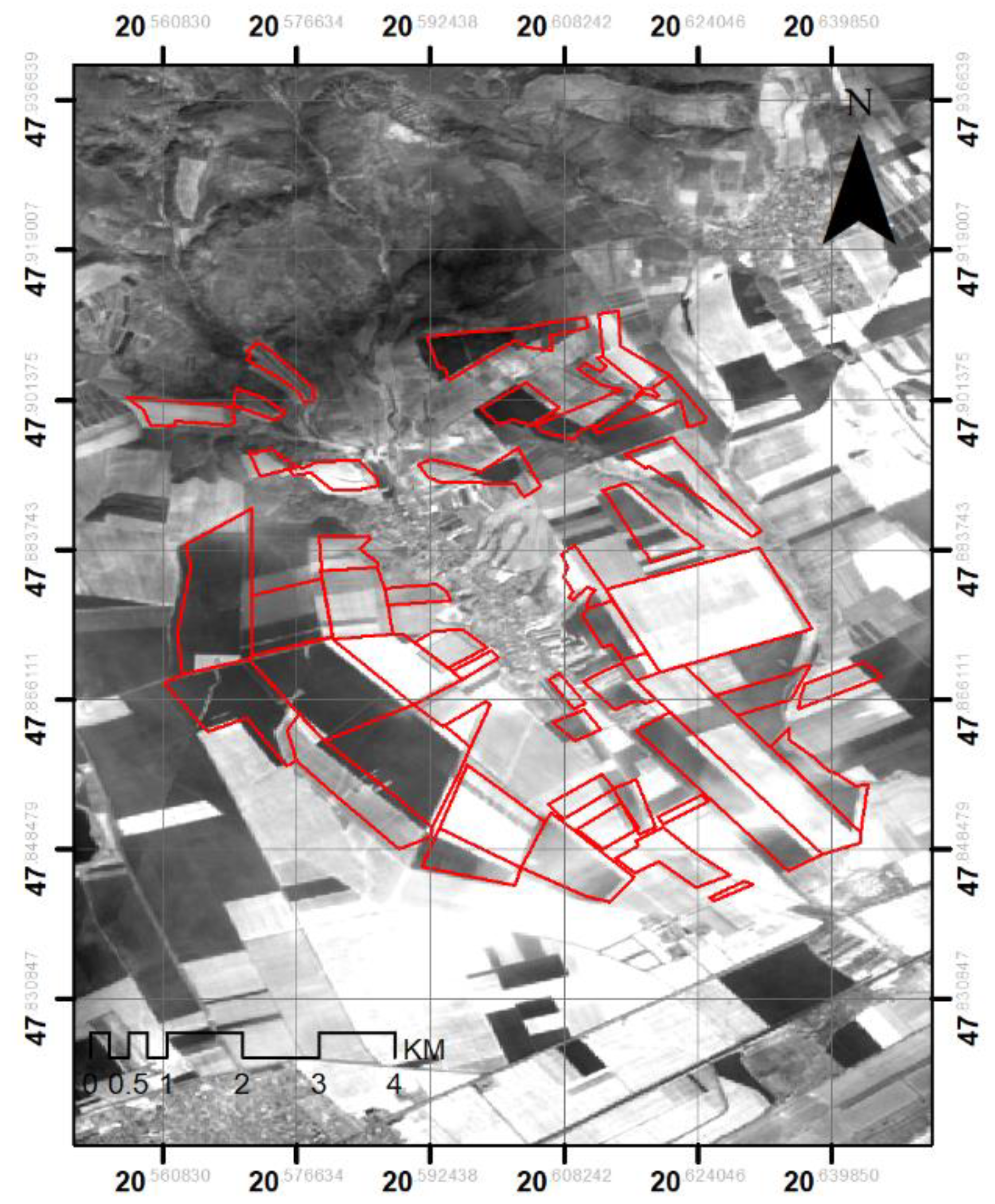
The Sentinel-1 satellite of the European Space Agency (ESA) provides C-band images in both singular and dual polarization within a 12-day cycle. In this study, Sentinel-1B satellite imagery (Figure 3) was utilized to estimate soil moisture (Table 1). Hosseini et al. [35] suggested the use of co-polarized backscatter coefficients that transmit-receive polarization (VV) as they are less sensitive to system noise and cross-interference than the weaker cross-polarized coefficients (i.e., HV and VH). Then, to have coherence during soil moisture sensor modelling, the Synthetic Aperture Radar (SAR) data acquisition date was downloaded and the dates that matched with the field measurement data were chosen, i.e., measured soil moisture date and time (2 a.m.). Although this time (2 a.m.) was different to each satellite passing time, the chosen time showed a consistent night reading that did not have any influence on temperature, which plays an important role the soil moisture calculation.
3.1.3. Landsat 8 Imagery
Landsat 8 was launched in 2013, and the Operational Land Imager (OLI) provides high-quality multispectral images at the resolution of 30 m (15 for panchromatic) and a revisiting time of 16 days. Four Landsat 8 images were downloaded for January, February, May, and June (Table 2). The dates of the measured soil moisture were matched to the closest acquisition date of the Landsat 8 image. The NDVI values were then calculated from the Landsat 8 image.
3.2. Methods
3.2.1. Data Collection and Retrieval of Measured Soil Moisture
Data were collected weekly in the field using a 2-step synchronization process. Firstly, to collect data from the sensor, it was connected to the flower power app installed on a smartphone or tablet via Bluetooth. Then, as soon as a connection was established, data collection started automatically. Secondly, the collected data were then uploaded to the cloud (data synchronization). For this step, an internet connection (3G or Wi-Fi) was required.
Finally, data were downloaded from the cloud into an excel CSV file that was then checked for any anomalies. If any anomalies were found, at a specific time, the data point was deleted from the raw data set. Examples of anomalies included missing data as the sensor failed to record, and abnormal readings mainly caused by low batteries or crackling disturbance. In this study, less than 5% of the data contained anomalies; therefore, the measured data were suitable for analysis.
The environmental covariates were selected partly by expert decision, and Sentinel-1 and NDVI data were chosen as target explanatory variables to integrate. Digital terrain data and terrain covariates were selected based on the best correlation with field SM observation.
3.2.2. Extraction of Covariates
A combination of literature and statistical processing was used to select several covariates. Based on the literature, covariates had to meet three criteria; firstly, they had to represent the soil-forming factors; secondly, they had to have a direct relationship with SM; and thirdly, they had to be commonly accessible [34]. Based on these requirements, three kinds of data were chosen as environmental covariates, Sentinel-1 C-band, terrain data derived from DEM, and normalized difference vegetation index (NDVI) data to explain the biomass/vegetation influence on the SM [36]. Unfortunately, all the available dates for the Sentinel-2 data had cloud cover, so NDVI data were downloaded from Landsat 8, which provides seasonal coverage of the global landmass at a spatial resolution of 30 m (visible, NIR, SWIR). As there are a large number of environmental covariates that can be derived from a DEM, only a few were selected that had a direct relationship with soil moisture. The environmental covariates were statistically tested through a Pearson correlation (Table 3) to determine which covariates had the highest correlation with soil moisture (Figure 4). The three covariates that had the highest significance were slope, aspect, and relief.
The DEM of the entire study area was extracted from the 1:10 000, EU-DEM using the clipping tool in ArcGIS [37]. The most important parameter of this study was the DEM because three environmental covariates were derived from it. The first environmental covariate derived from the DEM was the slope. The slope had an impact on the runoff of surface water, infiltration rates, and even the rate of erosion, all of which are key to the soil moisture analysis. In ArcGIS, the slope was calculated using the Spatial Analyst Tools/Surface/Slope using the DEM as the input raster. The tool identifies the slope (gradient, or rate of maximum change in z-value) from each cell of a raster surface.
The next environmental covariate derived was the aspect ratio. The direction of the slopes affects the soil moisture content of the soils. For example, areas with southern slopes were mostly exposed to the sun’s radiation energy, making their surface level drier. In contrast, the northern slopes appeared to be slightly wet, and more humid. The aspect was derived using the Spatial Analyst Tools/Surface/Aspect.
The relief intensity “RI” is one of the commonly used environmental covariates of surface characterization, which gives the differences between the highest and lowest points within a given unit of territory, that is, the amount of potential energy. Its value is usually expressed in m km−1. Due to the small size of the study area, we calculated a circle of a 500-m diameter with the help of the “focalrange” command in the Focal Statistics toolbox within ArcGIS.
We also decided to add the flow-accumulation/contributing area as the fourth variable, because this derivative explains the surface water flow and potential redistribution of the surface water and soil moisture along the slope. Its potential impact on the SM estimation is evident, especially in this very clayey area, where the surface water movements are very significant.
Flow accumulation was calculated using the following steps: The first step in ArcGIS (using a DEM as an input raster) was to create a DEM that is depressionless or hydrologically corrected. This step was completed using the FILL command in ArcGIS that fills all the sinks and ensures all chances of differentiation on the plain areas are minimized. However, instead of filling all sinks, it is important to introduce a sink depth limit that will be used as the limit value. Any sink deeper than the specified limit will be kept untouched. The second step was to create the flow direction, which was created by the FLOW DIRECTION function to create a grid/image of flow. It was calculated based on the following formula:
Drop = (∆Elevation/Cell centre distance) × 100.
Then, based on the flow direction grid, the size of the contributing area to each grid cell was calculated with the FLOW ACCUMULATION function of which the output grid file represented the catchment area size of each grid cell expressed as cell counts. The third step involved applying a threshold value to the flow accumulation grid to create a stream network. All cells, which had a contributing area higher than a particular threshold value, were assigned a value of 1, representing the drainage path. All other cells, which had a flow accumulation value below the threshold, were assigned “no data” and became background cells [38].
The geology mainly defines the terrain of this study site, and there is a dominating NW-SE direction valley and range system, which explains the high importance of the aspects. The agricultural area has heavy clay and loamy sand textures. The heavy clay covers the interfluves/plateaus, while the valley slopes with higher gradients are mainly sandy materials underlying the clay strata and exposed by erosion of the covering clay. Therefore, the terrain explains much of the soil parent material changes and soils types as well. Of course, this correlation is valid only locally, but these kinds of locally valid terrain factors can be derived in other areas with a comparatively small size. Similar terrain data can be derived from precision farming machinery data, so the approach can be applied easily anywhere, where precision farming with real-time kinematic (RTK) navigation is used.
3.2.3. Pre-Processing and Selection of Sentinel 1 Imagery
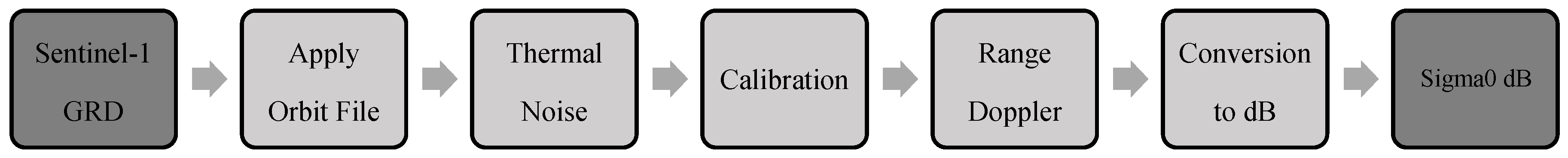
The Sentinel-1B image Ground Range-Detected (GRD) product was chosen because Level-1 GRD products consist of focused SAR data that has been detected, multi-looked, and projected to ground range using an Earth ellipsoid model as opposed to a single look complex (SLC). The ellipsoid projection of the GRD products is corrected using the terrain height specified in the product general annotation. Then, downloaded Sentinel 1 images were subjected to analysis to remove noise from the images that would affect the finial backscatter coefficient. The analysis was performed using specifically designed steps for pre-processing (Figure 5), which included apply orbit file, thermal noise removal, calibration, and terrain correction [39], which were accomplished using SNAP software version 7.03. These steps were followed to obtain a Sigma “σ” backscatter coefficient. Then, the unitless backscatter coefficient is converted to σ(dB) using a logarithmic transformation using the following formula [40]:
where by DN is a raw digital number.
σ (dB) = log10(DN),
Apply Orbit
The process of applying a precise orbit available in SNAP allowed the automatic download and updating of the orbit state vectors for each SAR scene in its product metadata, providing an accurate satellite position and velocity information for each image.
Thermal Noise Removal
Sentinel-1 image intensity was disturbed by additive thermal noise, particularly in the cross-polarization channel. Thermal noise removal reduced noise effects in the inter-sub-swath texture, within the entire Sentinel-1 scene and resulted in a reduction of discontinuities between sub-swaths for particular normalization of the backscatter signal scenes in multi-swath acquisition modes [41].
Calibration
Calibration was the procedure that converted digital pixel values to radiometrically calibrated SAR backscatter. The information required to apply the calibration equation was included within the Sentinel-1 GRD product; specifically, a calibration vector included as an annotation in the product allows simple conversion of image intensity values into sigma nought values. The calibration reverses the scaling factor applied during level-1 product generation and applies a constant offset and a range-dependent gain, including the absolute calibration constant [39].
Range Doppler Terrain Correction
Terrain correction was performed to compensate for distortions so that the geometric representation of the image will be as close as possible to the real world. Range Doppler terrain correction is a correction of geometric distortions caused by topography, such as foreshortening and shadows, using a digital elevation model to correct the location of each pixel [39]. The range Doppler terrain correction operator available in SNAP implements the range Doppler orthorectification method for geocoding SAR scenes from images in radar geometry. It makes use of available orbit state vector information in the metadata, the radar timing annotations, and the slant to ground range conversion parameters together with the reference digital elevation model data to derive the precise geolocation information [40].
Conversion of the Image to dB
As a last step of the pre-processing workflow, the unitless backscatter coefficient is converted to dB using a logarithmic transformation Equation (2). Finally, a raster image was created for each day that contained mean σ(dB) in VV, VH polarizations, and local incidence angles. These images were then used to derive soil moisture values.
The selection of Sentinel 1 images was selected based on the resultant image generated after the pre-processing steps. Raster images were visually analyzed in ArcGIS to see which images had the least “noise” interference after pre-processing. The noise was determined by the deviation of the pixel value per given test field. The land use of each test field was known, the change in pixels over each test field was analyzed, and the images with the best pixel arrangement were chosen. The Sentinel-1B images that had minimal noise and adequate backscatter coefficients values were acquired on four dates: 30 January, 2 February, 10 May, and 6 June 2019.
3.2.4. Spatial Interpolation Methods
In this study, three interpolation methods were used to describe and analyze the predicted soil moisture. The geostatistical interpolation methods used were multiple linear regression, regression kriging, and cokriging. Kriging is a type of stochastic model that characterizes the unknown spatial variability, the magnitude of which is described with variance [42].
Multiple Linear Regression (MLR)
MLR is capable of predicting soil properties with multispectral data. In this study, MLR was used to describe and model the relationship between environmental covariates (explanatory variables) and the observed soil moisture, and a 0.01 significance was applied. The predicted value of the regression model contained an error component, which showed the difference between the predicted value and the observed value of the data point.
Regression Kriging (RK)
Regression kriging (RK), also termed universal kriging or kriging with an external drift, combines regression of the target variable on environmental covariates with kriging of the regression residuals [31]. RK is the sum of prediction from MLR and ordinary kriging of the regression residuals. The advantage of RK is the ability to extend the method to a broader range of regression techniques and to allow a separate interpretation of the two interpolated components [43].
Cokriging (CK)
Cokriging is a function of ordinary kriging, which uses two or more variables to estimate or predict a primary variable. Cokriging usually reduces the prediction error variance and specifically outperforms the kriging method if the second variable is highly correlated with the primary variable [44]. In this study, three selections of cokriging where chosen: DEM + Sentinel, NDVI + Sentinel, and DEM + Sentinel + NDVI.
3.2.5. Estimation of Soil Moisture
Estimation of soil moisture involved the testing of empirical models to present a correlation between measured soil moisture and predicted soil moisture derived from environmental covariates and backscattering coefficients with the aid of the ordinary least square (OLS) linear regression function [45]. Many researchers established empirical relationships to estimate soil moisture, and these models revealed that there is a fundamental relation between soil moisture and the backscattering coefficient [45,46,47,48,49].
First, an empirical model based on the influence of the slope, aspect, relief, surface flow accumulation, backscatter coefficient in the VV polarization, and NDVI were developed. We considered in situ soil moisture as a function of the variables mentioned above, as seen in Equations (3) and (4):
where “slp” is the slope, “aspct” is the aspect, “rel” is relief intensity, “flacc” is flow accumulation, “σVV” is the backscatter coefficient, “NDVI” is the vegetation index, and “a” is an intercept and, b,c,d,e,f,g are coefficients derived from the OLS linear regression function in ArcGIS. In this multiple linear regression, mv (soil moisture in vol %) is the resultant predicted soil moisture value, and slope, aspect, relief, flow accumulation, and backscatter coefficient are functions in the regression model Equation (3).
mv = f(slp, aspct, rel, flacc, σVV, NDVI),
mv = a + b×slp + c×aspct + d×rel + e×flacc + f×σVV +g×NDVI,
The terrain variable layers were overlain by the point shapefile of the parrot observations, and the corresponding values from all layers were extracted into a data vector file. This point output file was used to calculate the coefficients for the regression model which were later used to estimate the SM values using the “Raster Calculator” in ArcGIS Equation (4). The output raster file was the predicted soil moisture value as a percentage (vol %) for the particular chosen time (January, February, May, and June).
The errors of the regression prediction for the observation sites were calculated and used in an ordinary kriging procedure to estimate the error over the entire area. The regression results and the error estimation were summed up to have an error corrected estimation map, where the RMSE was used to evaluate the results.
Cokriging was performed using the procedure of regression kriging, but three covariates were used as secondary inputs into the model: DEM, the Sentinel-1B C band, and NDVI. The results were compared and analyzed using the RMSE.
3.2.6. Validation of Soil Moisture
This paper did not aim to validate the sensor data as it was already done by [3]. In real CO, soil moisture estimations come from different sensors and different calculation methods that introduce much inconsistency to the dataset, which is one of the significant limitations of the CO approach. In this study, we aimed to validate the estimation procedure only. Cross-validation requires a larger amount of data. Our study area was relatively large compared to the number of sensors, so each sensor contributed significantly to the estimation process. The split of the dataset to the modelling and testing datasets would have dramatically decreased the performance. Therefore, we used only the RMSE value derived from the model development and the leave-one-out cross-validation method of the ArcGIS.
The selection of the optimal day of each month was based on the Sentinel 1 image availability that had the “least border noise effect” during the month. The accuracy assessment of the regression model was conducted in ArcGIS, and the statistical metrics, namely R2 and RMSE, were determined, as shown in Table 4. The regression kriging and cokriging results were generated with the geostatistical toolset of ArcGIS. The results are presented monthly for four months, and they are differentiated into two groups: “all land uses” and “wheat land use”.
4. Results and Discussion
Two images are presented in Figure 6 to visually study the sensor values having the DEM as a background to both images. The image from February 2019 represents a dry period, while June 2019 shows the wet conditions. The dry values occur mainly in the northern part of the images, because of the water seepage downward following the southern sloping nature of the pilot area. In the dry period, the valleys are drier, because their texture is coarser, loamy, and sandy, which retains much less moisture than the clayey material of the plateaus. In contrary, the wet period shows a different picture. The valley bottom becomes wetter due to the accumulating water from the surface runoff. At the same time, the plateaus stay a little bit drier due to the slow and limited infiltration into the clayey material. However, there is some indifferent unexplained variability of the measured values that do not match the overall terrain and soil trends. These are due to short-range micro terrain variability not shown by the DEM or to the differences in the soil properties that we could not map at this scale. This unexplained variability ranges between the 3% and 10% absolute value, with an average of around 5%, which remains unexplained by our models as well, the RMSE for the models, which were found to be in the same range.
It should be noted that the upper 10-cm layer usually dries very quickly and remains dry. As such, the results presented below are not fully representative of the entire soil profile, namely the deeper horizons of the soils. The conditions of the upper 10 cm are spatially much more homogeneous, and they do not necessarily reflect the differences between the different soil types and terrain locations, which limits the performance of the modelling exercise. Despite its identified limitations, we believe that the CO data contains useful information, explains the major trends, and is worthy for testing as inputs for SM estimation procedures.
Table 3 shows the best for terrain variables and the Pearson’s coefficient. The values range between 0.45 and 0.62. These values are similar to [27], who recorded values of the Pearson correlation coefficient (R) ranging from 0.58 to 0.81 for four different vegetation covariates extracted from the MODIS dataset.
4.1. Multiple Linear Regression (MLR)
In this study, a multiple linear regression model was used first to estimate soil moisture in the upper 10 cm of the soil profile. The resulting equations are shown in Table 4, while the summary table of the generated statistics is presented in Table 5, which showed the model failed to cover the entire range of the observed values.
The measured soil moisture statistics describe the soil moisture trend of the study period (Table 5). The January and February dates have low, but not extremely low, values with greater variance. The small rain incident did not saturate the entire area, and the impact of different soil types and terrain created a variable SM due to the soil-terrain factor differences. The standard deviation was the highest in January, followed by high values in February and June, which made it easier for the estimation framework because a lot of the variability could be explained by our variables when the biomass cover was still low. May was the wettest time with the highest mean and the lowest range, meaning a more or less wet soil condition in the whole area. The soils started to dry out in June, due to the hot summer weather, high evaporation, and transpiration of the large biomass and the decreasing precipitation. The model results of MLR (Table 6) showed an R2 value range of 0.19 to 0.25 in the category of “all land uses” whereas in the category of “wheat”, it ranged from 0.28 to 0.35. The RMSE ranged from 5.86 to 4.14 in the category of “all land uses” whereas in the category of “wheat”, it ranged from 4.76 to 3.77. This highlights that the model is better at predicting soil moisture in one land use as opposed to many land uses. Additionally, the RMSE agrees with the literature on satellite backscatter coefficients, indicating the different types of land use significantly affect the independent variable (backscatter coefficient) of the model. As a result, RMSE values of >3 are usually achieved [23].
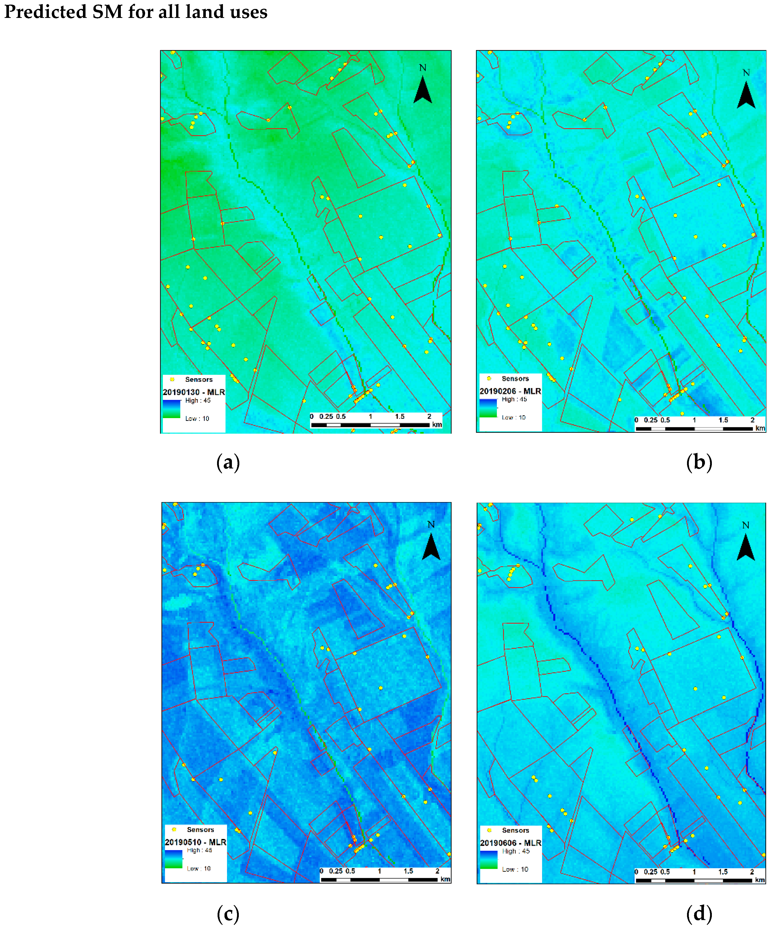
The interpretation of the spatial structure of the predicted SM images describes the weather trends and the redistribution of the SM due to the soil-landscape processes well. Figure 7 and Figure 8 show four SM images of the study area using the same color scheme. We had a dry January, a little bit wetter though dry February. May and June were wetter with high precipitation, with increasing evapotranspiration due to the high biomass and the warming summer weather. This means the water balance changed by June from positive to negative, and the area started to dry up. This process is evident, with the reintroduction of the greenish colors on the northern part of the image resulting in a textbook-like example of SM redistribution due to water seepage flowing to the southern sloping terrain of the foothill area/s and the drying of the plateaus, while the lower parts of the slopes are still wet (Figure 7c,d and Figure 8c,d).
The two sets of images are so different because the “all land uses” images (Figure 7) are well adjusted to the terrain, due to the more general and variable land use sampling, so the land use effect is “dissolved”. While the images in Figure 8, where only the wheat land use was sampled, show a strong misleading impact of the land use. The strong blue areas of Figure 8a and the green ones of Figure 8c are not necessarily due to higher or lower soil moisture, and they mainly represent the pastures, forests, and orchards, and the non-agricultural areas around the village. This comparison makes it clear that the resulting maps can be interpreted only within the same class or classes that were sampled, which in our case is only the area delineated by the parcel polygons on the images. The general conclusion is that the resulting images show a very realistic spatial pattern for the sampled areas in both land uses (Figure 7) but more so in the wheat land uses (Figure 8), which matches the expert judgements, but the value ranges are significantly lower. The model overestimates the low values, while it underestimates the high ones and matches around the mean. The smoothing impact on the image explains the good realistic spatial patters, but the values are increasingly over- and underestimated towards the extremes.
4.2. Regression Kriging
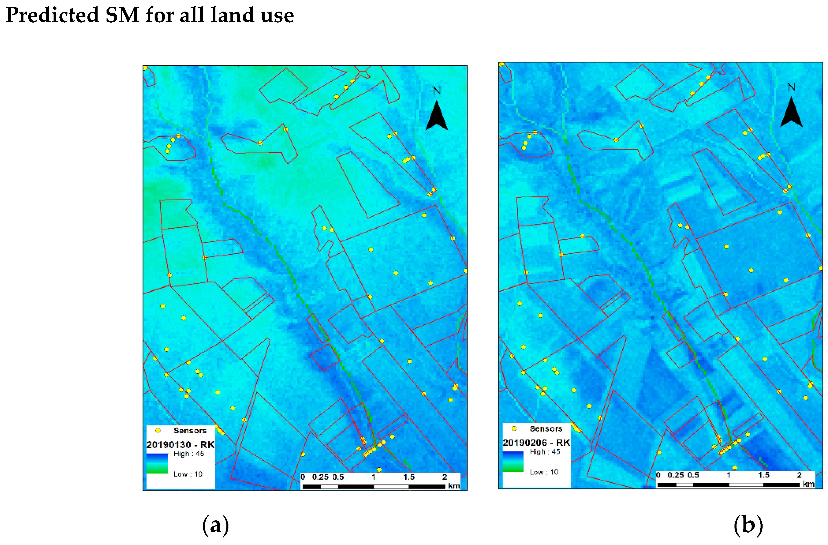
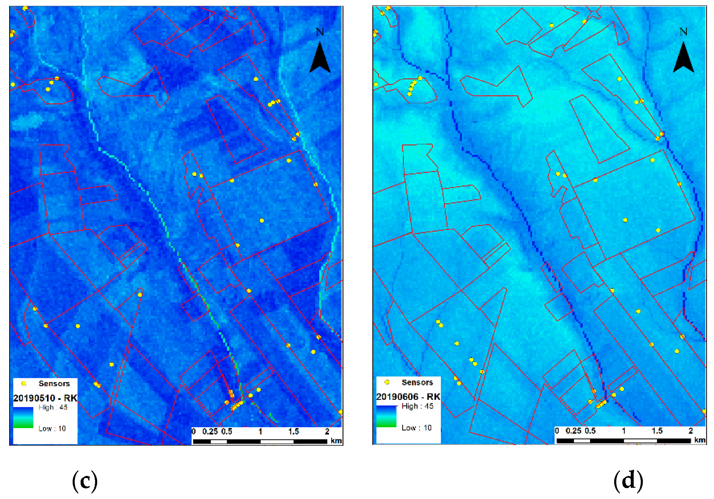
The MLR results presented a good spatial structure and resulted in relatively average RMSE (Table 6) values, which meant that the deterministic part of the described variability by the model was fair. In order to decrease the deviation from the observed values and try to explain the stochastic part of the spatial SM variation, the errors for all observation sites for each of the dates were calculated and krigged to develop continuous layers of error distributions over the study area. The values of these layers were added to the regression results to correct the deviation from the observed values. This approach is very similar to running an ordinary cokriging approach, where the trend is modelled by the linear regression, and the error is krigged. The leave-one-out cross-validation approach was used to describe the results that are shown in Table 7. The comparison of the results of the linear regression (Table 6) and the error kriging results (Table 7) shows a significant refinement of the estimations. This approach decreased the RMSE of the linear regression model for all cases, keeping the realistic spatial structure (Figure 9 and Figure 10), which reveals the terrain and soil conditions. It is noted that this refinement is very dependent on the sampling density and the representativity of the spatial sampling design to the stochastic factors of the area.
4.3. Ordinary Cokriging
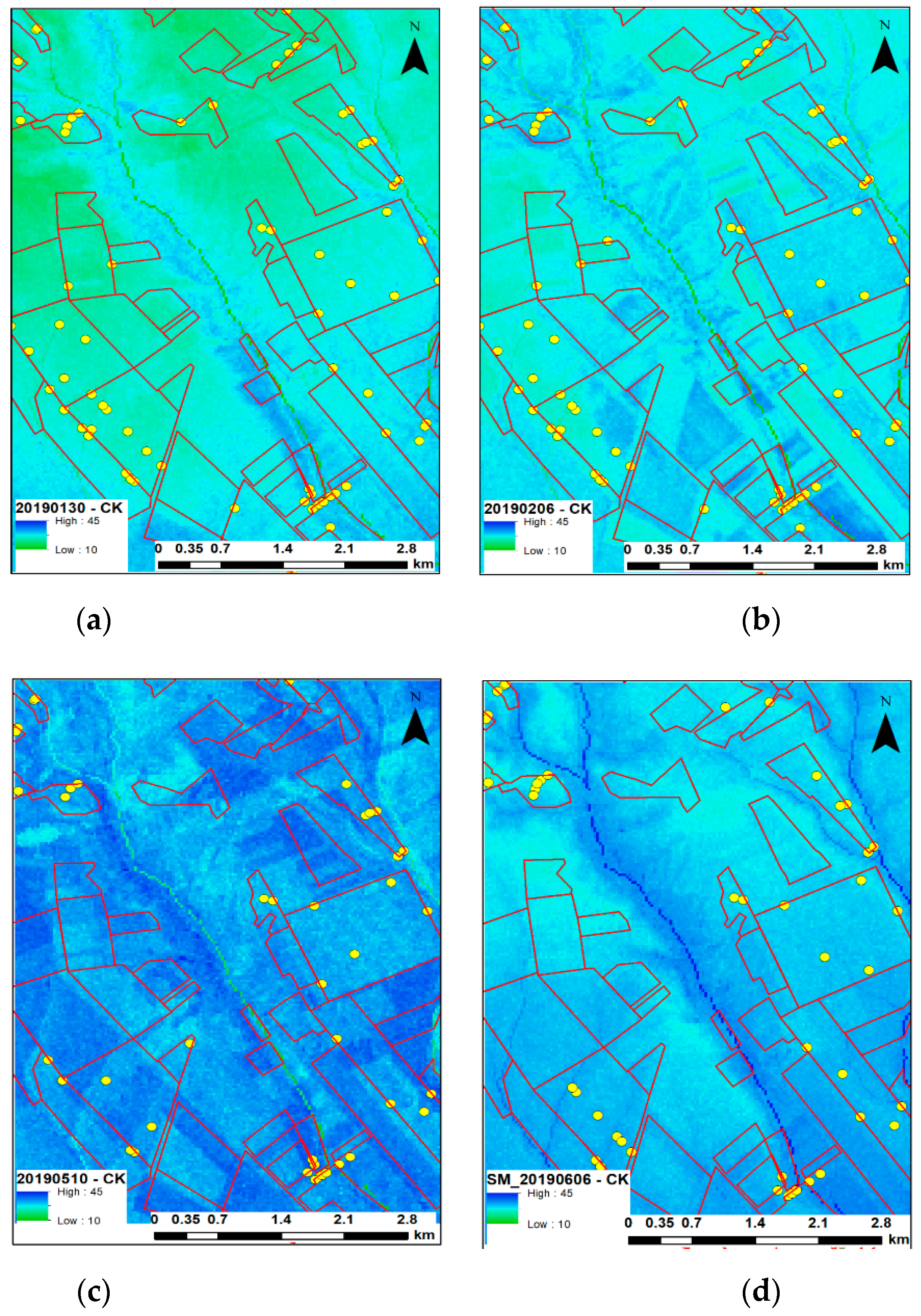
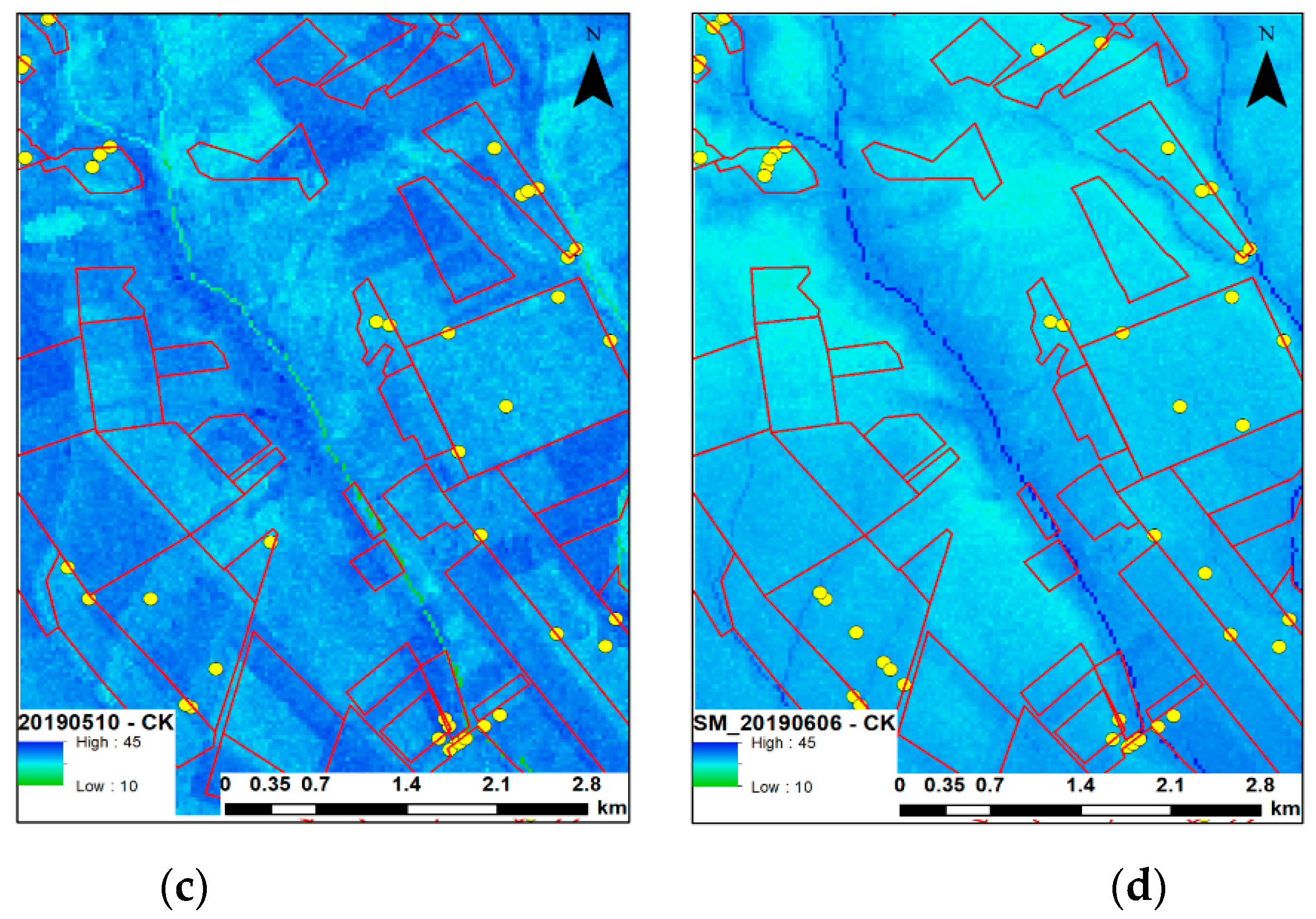
Cokriging using the ordinary kriging method with three different covariate setups—DEM + Sentinel, NDVI + Sentinel, and DEM + Sentinel + NDVI—was done for the four dates and two land use classes. The statistical measures of the results are presented in Table 8. In general, the cokriging performed significantly worse than the regression kriging and a little bit worse than the multiple linear regression approach. The RMSE values were found to be very similar for the two classes on all dates, and no significant difference was found between the setups (Figure 11). For January and May 2019, the cokriging yielded slightly better results in the wheat land use class as opposed to the all land use class (Figure 12). On the contrary, for February and June 2019, the cokriging increased the performance of the model of only the “all land use” class, and the wheat class performances were always slightly worse. One of the potential explanations comes from the lower number of observation sites. Kriging or any spatial interpolation method requires a fair density of the observation sites covering the representative points of all geomorphologic soil-landscape units. Any gap in the observation network will result in unrealistic estimation if real spatial autocorrelation between the neighboring points does not exist. The regression approach is not as sensitive; it works on a point vector basis. This is why it performs better in a very limited data density scenario. The sampling was parcel based, and the parcels were distributed over the landscape, often far from each other. Therefore, clear spatial relationships were not always detectable between the points, especially considering the large target–within-field scale.
The best results for the “all-land use” class were mainly the NDVI + Sentinel supported cokriging, while the best case for the wheat class was always the NDVI-DEM-Sentinel setup. However, the differences between the three different setups were not much in both classes, meaning that the covariates used in the cokriging procedure could not add much extra information to the kriging-based estimation.
4.4. Comparison of the Results
Table 9 presents the results of the three different approaches that were developed and tested, showing the RMSE values, which were compared per monthly per land use to determine the best approach per month. The overall findings for each approach are presented below:
(1) Multiple linear regression performed relatively well in comparison to the cokriging approach, especially when the results were corrected using the krigged error layers, namely the regression kriging approach. The linear regression model provided a very realistic SM distribution over the landscape that matches with the known driving forces of the SM distribution, where the RMSE ranged from 3.77 to 5.85. The results match with the ones published by [29]. The R2 values ranged between 0.19 and 0.35, which are quite low, but more or less match the literature results at this scale. This was similar to [29], who reported an R2 of 0.24. It was mainly because the model was overestimating the low values and underestimating the high ones and therefore decreased the range of the estimated values down to approximately 60% of the measured values. The major advantage of this approach was that it is less sensitive to the number of data points and the data density.
Many SAR analysis and modelling studies have relied on the coefficient of determination (i.e., R2) statistics, and in some cases, considering R2 = 0.30 as the threshold criteria for accepting a given model for reliable estimation and prediction [20]. The corresponding literature of the use of SAR data for SM estimation reported R2 values of 0.24 [29], 0.4 to 0.58 [23], and up to 0.71 [24]. However, the study setups—climate, vegetation cover and the used covariates, the accuracy and reliability of the used sensors—are so different, and it is not easy to compare the numbers alone. The low R2 values often reported in the scientific reports suggest that the SM variability has a lot of short-range variabilities. This could be attributed to the complex physical nature of soils and the unpredictable impacts of the strongly variable vegetation and cropping techniques that are still not explained by our models.
(2) Regression kriging (RK) is one of the most popular spatial interpolation techniques in soil science [26]. The regression kriging results showed that the proposed empirical model predicted the soil moisture content with the RMSE range of 1.30 to 4.39, depending on the standard deviation of the measured values, which was considered acceptable considering the sample size deployed, and area mapped. In order to explain the unexplained stochastic component of the variation, the error values on the observation sites were calculated and krigged over the study area, assuming a spatial dependence structure in the values driven by some unexplained factors of the landscape. These values were used to correct the regression estimation, and the process was validated with the leave-one-out cross-validation approach. The calculated RMSE values were significantly lower for all cases and often resulted in a considerable accuracy improvement. However, it has to be noted here that this improvement in the statistics is very dependent on the spatial setup and representativity of the sampling design, and does not always correct the error evenly over the landscape and land uses.
(3) The ordinary cokriging results showed the weakest performance, with not much traceable impact of the covariates applied in our study, which could be attributed to the low impact of combined covariates on the kriging approach. There is a rich literature on the use of kriging to interpolate soil moisture data. Zhang et al. [30] reported RMSE values between 2.62 and 3.01 using different kriging approaches, like ordinary, cokriging, and extended kriging. Zeng et al. [28] reported RMSE in the same range, but this study was performed on a bare soil surface, lacking the vegetation effect on the estimation. Gharechelou et al. [25] reported even better RMSE for an arid area, where the original value range was between 0% and 10% SM. They found the RMSE to be around 1.8. In our study, the range was between 10 and 40, so the relative deviation compared to the range is equal.
5. Conclusions
In this study, three statistical models were developed to map soil moisture content using Sentinel-1B C-band SAR satellite data, NDVI, and terrain information. Multiple linear regression, regression kriging, and ordinary cokriging were tested for quick SM mapping using low-cost sensor data from CO, where the sensors were deployed into the topmost 10 cm of the soil. This layer experiences a strong weather exposure/influence together with a strong vegetation and farming effect. It dries out and become wet quite quickly, depending on the weather conditions, and is more exposed and sensitive to weather conditions than to the soil and terrain position. Despite this presumption, the expert knowledge-based interpretation of the data values over the terrain and soil properties found the data distribution matched with the factors driving the SM variability over the landscape relatively well.
Based on the above statements and findings, linear regression provides more realistic spatial patterns over the landscape, even in a data-poor environment. Regression kriging was found to be a potential tool to refine the results, while ordinary cokriging was found to be less effective. In relation to our aim of whether CO data can be used as a reliable source, it was concluded that the CO data has a real potential to provide inputs for temporal SM mapping using easy-to-access freely available datasets, like DEM and Sentinel-1 and Landsat 8 data. The RMSE values of the regression kriging are comparable or even better than the values reported for similar digital soil mapping approaches, between 1.3 and 4.39, while the literature-reported values often go above. The trends were always well identified by the models, but the value ranges were always lower than the original values. The data represent the major SM distribution trends over the landscape, but there is still a significant amount of variability that cannot be interpreted by local expert knowledge in the given resolution of the covariates.
In general, the data produced by the CO-based low-cost sensors were found to be appropriate for SM mapping, mainly to interpret the spatial SM distribution over the landscape. No negative deviation from the reported values of similar studies using professional devices and field setups was identified, so the low-cost sensor data from CO networks can provide valuable data for SM mapping. The positive finding was that the trend describing the more and less moist areas are well explained, while the deviations of the estimation from the observed values increased towards the extremes. In order to fully understand these trends, further studies are needed on the functionality of overestimating and underestimating predicted values.
Author Contributions
Conceptualization, D.K. and E.D.; methodology, D.K. and E.D.; software, D.K.; formal analysis, D.K. and E.D.; investigation, D.K.; writing—original draft preparation, D.K.; writing—review and editing, D.K. and E.D.; visualization, E.D.; supervision. All authors have read and agreed to the published version of the manuscript.
Funding
This research received no external funding.
Acknowledgments
The research was carried out within the GINOP-2.3.2-15-2016-00031 “Innovative solutions for sustainable groundwater resource management” project of the Faculty of Earth Science and Engineering of the University of Miskolc in the framework of the Széchenyi 2020 Plan, funded by the European Union, co-financed by the European Structural and Investment Funds. The authors want to thank European Commission-supported “Grow” H2020 project (Project ID: 690199) for the materials used in this study, expert advice on soil science and making this knowledge available to many people from different facets of life. The described article was carried out as part of the EFOP-3.6.1-16-2016-00011 “Younger and Renewing University—Innovative Knowledge City—institutional development of the University of Miskolc aiming at intelligent specialisation” project implemented in the framework of the Szechenyi 2020 program. The realisation of this project is supported by the European Union, co-financed by the European Social Fund.”
Conflicts of Interest
The authors declare no conflict of interest. The funders had no role in the design of the study; in the collection, analyses, or interpretation of data; in the writing of the manuscript, or in the decision to publish the results.
References
- Bablet, A.; Viallefont, F.; Fabre, S.; Briottet, X.; Jacquemoud, S. Assessment of Soil Moisture Content Using a Multilayer Radiative Transfer Model of Soil Reflectance (MARMIT) in the Solar Domain. Geophys. Res. Abstr. 2018, 20, 17709. [Google Scholar]
- Entekhabi, D.; Njoku, E.G.; O’Neill, P.E.; Kellogg, K.H.; Crow, W.T.; Edelstein, W.N.; Van Zyl, J. The Soil Moisture Active Passive (SMAP) Mission. Proc. IEEE 2010, 98, 704–716. [Google Scholar] [CrossRef]
- Kovács, K.Z.; Hemment, D.; Woods, M.; Van Der Velden, N.K.; Xaver, A.; Giesen, R.H.; Burton, V.J.; Garrett, N.; Zappa, L.; Long, D.; et al. Citizen Observatory Based Soil Moisture Monitoring—The Grow Example. Hung. Geogr. Bull. 2019, 68, 119–139. [Google Scholar] [CrossRef]
- Dorigo, W.A.; Oevelen, P.; Wagner, W.; Drusch, M.; Mecklenburg, S.; Robock, A.; Jackson, T. A New International Network for in Situ Soil Moisture Data. Eos Trans. Am. Geophys. Union 2011, 92, 141–142. [Google Scholar] [CrossRef]
- Dorigo, W.A.; Wagner, W.; Hohensinn, R.; Hahn, S.; Paulik, C.; Xaver, A.; Robock, A. The International Soil Moisture Network: A Data Hosting Facility for Global in Situ Soil Moisture Measurements. Hydrol. Earth Syst. Sci. 2011, 15, 1675–1698. [Google Scholar] [CrossRef] [Green Version]
- Indian People Organizing for Change. Climate Change 2007: The Physical Science Basis. Agenda 2007, 6, 333. [Google Scholar]
- Xaver, A.; Zappa, L.; Rab, G.; Pfeil, I.; Vreugdenhil, M.; Hemment, D.; Dorigo, W.A. Evaluating the Suitability of the Consumer Low-Cost Parrot Flower Power Soil Moisture Sensor for Scientific Environmental Applications. Geosci. Instrum. Methods Data Syst. 2020, 9, 117–139. [Google Scholar] [CrossRef] [Green Version]
- Freitag, A.; Meyer, R.; Whiteman, L. Strategies Employed by Citizen Science Programs to Increase the Credibility of Their Data. Citiz. Sci. Theory Pract. 2016, 1. [Google Scholar] [CrossRef]
- Pocock, M.J.O.; Tweddle, J.C.; Savage, J.; Robinson, L.D.; Roy, H.E. The Diversity and Evolution of Ecological and Environmental Citizen Science. PLoS ONE 2017, 12, e0172579. [Google Scholar] [CrossRef]
- Gharesifard, M.; Wehn, U.; Van Der Zaag, P. Towards Benchmarking Citizen Observatories: Features and Functioning of Online Amateur Weather Networks. J. Environ. Manag. 2017, 193, 381–393. [Google Scholar] [CrossRef]
- Woods, M.; Hemment, D.; Ajates, R.; Cobley, A.; Xaver, A.; Konstantakopoulos, G. GROW Citizens’ Observatory: Leveraging the power of citizens, open data and technology to generate engagement, and action on soil policy and soil moisture monitoring. In IOP Conference Series: Earth and Environmental Science; IOP Publishing: Bristol, UK, 2020; Volume 509, p. 012060. [Google Scholar]
- Al-Yaari, A.; Wigneron, J.-P.; Kerr, Y.; Rodríguez-Fernández, N.J.; O’Neill, P.E.; Jackson, T.J.; Yueh, S. Evaluating Soil Moisture Retrievals from Esa’s Smos and Nasa’s Smap Brightness Temperature Datasets. Remote. Sens. Environ. 2017, 193, 257–273. [Google Scholar] [CrossRef] [Green Version]
- Zhang, G.-L.; Liu, F.; Song, X.-D. Recent Progress and Future Prospect of Digital Soil Mapping: A Review. J. Integr. Agric. 2017, 16, 2871–2885. [Google Scholar] [CrossRef]
- McBratney, A.B.; Santos, M.M.; Minasny, B. On Digital Soil Mapping. Geoderma 2003, 117, 3–52. [Google Scholar] [CrossRef]
- Boettinger, J.; Howell, D.; Moore, A.; Hartelink, A.; Kienast-brown, S. Digital Soil Mapping; Springer Netherlands: Dordrecht, The Netherlands, 2010. [Google Scholar] [CrossRef] [Green Version]
- Bakker, A. Soil Texture Mapping on a Regional Scale with Remote Sensing Data. 2012. Available online: https://edepot.wur.nl/246954 (accessed on 24 July 2020).
- Jenny, H. Factors of Soil Formation. In A System of Quantitative Pedology, Soil Science; Dover Publications: Mineola, NY, USA, 1941. [Google Scholar]
- Rossiter, D.G. Digital Soil Resource Inventories: Status and Prospects. Soil Use Manag. 2006, 20, 296–301. [Google Scholar] [CrossRef]
- Malone, B.P.; Minasny, B.; McBratney, A.B. Digital Soil Mapping; Springer: Cham, Switzerland, 2017; pp. 1–5. [Google Scholar] [CrossRef]
- Zribi, M.; Albergel, C.; Baghdadi, N. Editorial for the Special Issue “Soil Moisture Retrieval using Radar Remote Sensing Sensors”. Remote Sens. 2020, 12, 1100. [Google Scholar] [CrossRef] [Green Version]
- Montanarella, L.; Pennock, D.J.; McKenzie, N.; Badraoui, M.; Chude, V.; Baptista., I. World’s Soils Are under Threat. Alice 2016, 2, 79–82. [Google Scholar] [CrossRef] [Green Version]
- Colliander, A.; Cosh, M.H.; Misra, S.; Jackson, T.J.; Crow, W.T.; Chan, S.; Bindlish, R.; Chae, C.; Collins, C.H.; Yueh, S.H. Validation and Scaling of Soil Moisture in a Semi-Arid Environment: Smap Validation Experiment 2015 (SMAPVEX15). Remote Sens. Environ. 2017, 196, 101–112. [Google Scholar] [CrossRef]
- Bousbih, S.; Zribi, M.; El Hajj, M.; Baghdadi, N.; Chabaane, Z.L.; Gao, Q.; Fanise, P. Soil Moisture and Irrigation Mapping in A Semi-Arid Region, Based on the Synergetic Use of Sentinel-1 and Sentinel-2 Data. Remote. Sens. 2018, 10, 1953. [Google Scholar] [CrossRef] [Green Version]
- Xing, M.; He, B.; Ni, X.; Wang, J.; An, G.; Shang, J.; Huang, X. Retrieving Surface Soil Moisture over Wheat and Soybean Fields during Growing Season Using Modified Water Cloud Model from Radarsat-2 SAR Data. Remote Sens. 2019, 11, 1956. [Google Scholar] [CrossRef] [Green Version]
- Gharechelou, S.; Tateishi, R.; Sharma, R.C.; Johnson, B.A. Soil Moisture Mapping in an Arid Area Using a Land Unit Area (LUA) Sampling Approach and Geostatistical Interpolation Techniques. ISPRS Int. J. Geo-Inf. 2016, 5, 35. [Google Scholar] [CrossRef] [Green Version]
- Keskin, H.; Grunwald, S. Regression Kriging as a Workhorse in the Digital Soil Mapper's Toolbox. Geoderma 2018, 326, 22–41. [Google Scholar] [CrossRef]
- Han, Y.; Bai, X.; Shao, W.; Wang, J. Retrieval of Soil Moisture by Integrating Sentinel-1A and MODIS Data over Agricultural Fields. Water 2020, 12, 1726. [Google Scholar] [CrossRef]
- Zeng, L.; Shi, Q.; Guo, K.; Xie, S.; Herrin, J.S. A Three-Variables Cokriging Method to Estimate Bare-Surface Soil Moisture Using Multi-Temporal, Vv-Polarization Synthetic-Aperture Radar Data. Hydrogeol. J. 2020, 1–11. [Google Scholar] [CrossRef]
- Chatterjee, S.; Huang, J.; Hartemink, A.E. Establishing an Empirical Model for Surface Soil Moisture Retrieval at the U.S. Climate Reference Network Using Sentinel-1 Backscatter and Ancillary Data. Remote Sens. 2020, 12, 1242. [Google Scholar] [CrossRef] [Green Version]
- Zhang, J.; Li, X.; Yang, R.; Liu, Q.; Zhao, L.; Dou, B. An Extended Kriging Method to Interpolate Near-Surface Soil Moisture Data Measured by Wireless Sensor Networks. Sensors 2017, 17, 1390. [Google Scholar] [CrossRef] [Green Version]
- Hengl, T.; Heuvelink, G.B.M.; Stein, A. A Generic Framework for Spatial Prediction of Soil Variables Based On Regression-Kriging. Geoderma 2004, 120, 75–93. [Google Scholar] [CrossRef] [Green Version]
- IUSS Working Group WRB (Ed.) World Reference Base for Soil Resources 2006. In World Soil Resources Reports; Food and Agriculture Organization of the United Nations: Rome, Italy, 2006. [Google Scholar]
- USDA-NRCS. Keys to Soil Taxonomy, 12th ed.; USDA-NRCS: Washington, DC, USA, 1998.
- Dobos, E.; Daroussin, J.; Montanarella, L. A Quantitative Procedure for Building Physiographic Units Supporting a Global Soter Database. Hungarian Geogr. Bull. 2010, 59, 181–205. [Google Scholar]
- Hosseini, R.; Newlands, N.K.; Dean, C.B.; Takemura, A. Statistical Modeling of Soil Moisture, Integrating Satellite Remote-Sensing (SAR) and Ground-Based Data. Remote Sens. 2015, 7, 2752–2780. [Google Scholar] [CrossRef] [Green Version]
- Dobos, E.; Michéli, E.; Baumgardner, M.F.; Biehl, L.; Helt, T. Use of Combined Digital Elevation Model and Satellite Radiometric Data for Regional Soil Mapping. Geoderma 2000, 97, 367–391. [Google Scholar] [CrossRef]
- EEA. Digital Elevation Model over Europe (EU-DEM). 2013. Available online: https://www.eea.europa.eu/data-and-maps/data/eu-dem (accessed on 1 April 2020).
- Dobos, E.; Daroussin, J. Calculation of Potential Drainage Density Index (PDD) Potential Drainage Density Index (PDD). In Digital Terrain Modelling; Springer: Berlin, German, 2007; pp. 283–295. [Google Scholar] [CrossRef]
- Filipponi, F. Sentinel-1 GRD Pre-processing Workflow . Proceedings 2019, 18, 11. [Google Scholar] [CrossRef] [Green Version]
- SNAP Software. SAR Basics Tutorial. 2019. Available online: http://step.esa.int/docs/tutorials/S1TBX%20SAR%20Basics%20Tutorial.pdf (accessed on 24 July 2020).
- Park, J.; Korosov, A.A.; Babiker, M.; Sandven, S. Efficient Thermal Noise Removal for Sentinel-1. IEEE Trans. Geosci. Remote Sens. 2017, 56, 1555–1565. [Google Scholar] [CrossRef]
- Dobos, E.; Carré, F.; Hengl, T.; Reuter, H.I.; Tóth, G. Digital Soil Mapping as a Support to Production of Functional Maps; EUR 22123 EN; Office for Official Publications of the European Communities: Luxemburg, 2006; p. 68. [Google Scholar]
- Hengl, T.; Heuvelink, G.B.M.; Rossiter, D.G. About Regression-Kriging: From Equations to Case Studies. Comput. Geosci. 2007, 33, 1301–1315. [Google Scholar] [CrossRef]
- Adhikary, S.K.; Muttil, N.; Yilmaz, A.G. Cokriging for Enhanced Spatial Interpolation of Rainfall in Two Australian Catchments. Hydrol. Process. 2017, 31, 2143–2161. [Google Scholar] [CrossRef] [Green Version]
- Sekertekin, A.; Marangoz, A.M.; Abdikan, S. Soil Moisture Mapping Using Sentinel-1A Synthetic Aperture Radar Data. Int. J. Environ. Geoinf. 2018, 5, 178–188. [Google Scholar] [CrossRef]
- Zribi, M.; Baghdadi, N.; Holah, N.; Fafin, O. New Methodology for Soil Surface Moisture Estimation and its Application to Envisat-Asar Multi-Incidence Data Inversion. Remote Sens. Environ. 2005, 96, 485–496. [Google Scholar] [CrossRef]
- Peng, J.; Loew, A.; Merlin, O.; Verhoest, N.E.C. A Review of Spatial Downscaling of Satellite Remotely Sensed Soil Moisture. Rev. Geophys. 2017, 55, 341–366. [Google Scholar] [CrossRef]
- Belenguer-plomer, M.A.; Chuvieco, E. Temporal Decorrelation of C-Band Backscatter Coefficient in Mediterranean Burned Areas. Remote Sens. 2019, 11, 2661. [Google Scholar] [CrossRef] [Green Version]
- Ezzahar, J.; Ouaadi, N.; Zribi, M.; Elfarkh, J.; Aouade, G.; Khabba, S.; Jarlan, L. Evaluation of Backscattering Models and Support Vector Machine for the Retrieval of Bare Soil Moisture from Sentinel-1 Data. Remote Sens. 2020, 12, 72. [Google Scholar] [CrossRef] [Green Version]
Figure 1.
Study area—Tard village located in the western county of Borsod-Abaúj-Zemplén in Hungary.

Figure 2.
Precipitation of the study area before and within the study period.

Figure 3.
Sentinel 1B imagery of Tard village with the parcels used for the study delineated in red. The specifications of Sentinel-1B data used in this study are listed below:
Figure 3.
Sentinel 1B imagery of Tard village with the parcels used for the study delineated in red. The specifications of Sentinel-1B data used in this study are listed below:

Figure 4.
(a) Digital Elevation Model (Metres Above Sea Level) and environmental covariates; (b) slope (degrees°); (c) aspect and (d) relief.
Figure 4.
(a) Digital Elevation Model (Metres Above Sea Level) and environmental covariates; (b) slope (degrees°); (c) aspect and (d) relief.

Figure 5.
Sentinel 1 ground range detection (GRD) pre-processing workflow, adapted from [39].
Figure 5.
Sentinel 1 ground range detection (GRD) pre-processing workflow, adapted from [39].

Figure 6.
(a) Mean soil moisture (V%) in February 2019—dry season and (b) mean SM (V%) in June 2019—wet season.
Figure 6.
(a) Mean soil moisture (V%) in February 2019—dry season and (b) mean SM (V%) in June 2019—wet season.

Figure 7.
All land use: Predicted soil moisture maps (V%)—(a) January 2019, (b) February 2019, (c) May 2019, and (d) June 2019, respectively.
Figure 7.
All land use: Predicted soil moisture maps (V%)—(a) January 2019, (b) February 2019, (c) May 2019, and (d) June 2019, respectively.

Figure 8.
Wheat land use: Predicted soil moisture maps (V%)— (a) January 2019, (b) February 2019, (c) May, and (d) June 2019, respectively.
Figure 8.
Wheat land use: Predicted soil moisture maps (V%)— (a) January 2019, (b) February 2019, (c) May, and (d) June 2019, respectively.

Figure 9.
All land uses: Error-corrected prediction regression kriging soil moisture map (V%)—(a) January 2019, (b) February 2019, (c) May 2019, and (d) June 2019, respectively.
Figure 9.
All land uses: Error-corrected prediction regression kriging soil moisture map (V%)—(a) January 2019, (b) February 2019, (c) May 2019, and (d) June 2019, respectively.


Figure 10.
Wheat land use: Error-corrected prediction regression kriging soil moisture map (V%)—(a) January 2019, (b) February 2019, (c) May 2019, and (d) June 2019, respectively.
Figure 10.
Wheat land use: Error-corrected prediction regression kriging soil moisture map (V%)—(a) January 2019, (b) February 2019, (c) May 2019, and (d) June 2019, respectively.

Figure 11.
All land uses: Ordinary cokriging soil moisture— (a) January 2019, (b) February 2019, (c) May 2019, and (d) June 2019, respectively.
Figure 11.
All land uses: Ordinary cokriging soil moisture— (a) January 2019, (b) February 2019, (c) May 2019, and (d) June 2019, respectively.

Figure 12.
Wheat land use: Ordinary cokriging soil moisture—January, February, May, and June 2019, respectively.
Figure 12.
Wheat land use: Ordinary cokriging soil moisture—January, February, May, and June 2019, respectively.


Table 1.
Specifications of the Sentinel-1B data used in the study.
| Specifications | Sentinel-1B |
|---|---|
| Acquisition times | January 2019–June 2019 |
| Imaging Mode | IW |
| Imaging frequency | C-Band (5.4 GHz) |
| Polarization | VV-VH |
| Data product | Level 1—GRD |
| Resolution mode | 10 m |
Table 2.
Landsat 8 acquisition dates.
| Measured Soil Moisture Acquisition Date | Landsat 8 Image Acquisition Date |
|---|---|
| 30 January 2019 | 21 January 2019 |
| 6 February 2019 | 6 February 2019 |
| 10 May 2019 | 13 May 2019 |
| 6 June 2019 | 14 June 2019 |
Table 3.
The Pearson’s correlation table of field SM data and the selected four terrain variables (2019 March data).
Table 3.
The Pearson’s correlation table of field SM data and the selected four terrain variables (2019 March data).
| Covariate | Pearson’s Correlation |
|---|---|
| DEM | 0.627 |
| Slope | 0.552 |
| Aspect | 0.489 |
| Relief | 0.571 |
Table 4.
Multiple Linear Regression Equations.
| Date | Intercept | Slope | Aspect | Relief | Flow Acc. | Sigma (σVV) | NDVI | No. of Observations |
|---|---|---|---|---|---|---|---|---|
| 30 January 2019 | 46.981453 | −0.020519 | 0.007187 | −0.004488 | −0.000907 | −0.337625 | −65.115101 | 76 |
| p value | 0.000000 * | 0.974165 | 0.628897 | 0.396057 | 0.561509 | 0.243762 | 0.430837 | |
| 6 February 2019 | 33.61278 | 0.031734 | −0.005617 | 0.000073 | −0.001149 | 0.30704 | 53.4524 | 76 |
| p value | 0.000001 | 0.953766 | 0.669784 | 0.988039 | 0.405165 | 0.130149 | 0.012407 | |
| 10th May 2019 | 47.490637 | −0.400499 | −0.014023 | −0.000658 | 0.000131 | 0.531087 | −3.42735 | 46 |
| p value | 0.000000 * | 0.461386 | 0.390445 | 0.896895 | 0.931458 | 0.05184 | 0.555235 | |
| 6th June 2019 | 47.719149 | −0.071528 | 0.000421 | 0.001496 | 0.000924 | 0.289084 | −3.045411 | 47 |
| p value | 0.000113 | 0.928151 | 0.982766 | 0.823476 | 0.60737 | 0.376018 | 0.804289 |
* indicates a coefficient is statistically significant p value (p < 0.01).
Table 5.
Statistics of measured and predicted soil moisture.
| Date | Min | Max | Mean | Standard Deviation | Range | |
|---|---|---|---|---|---|---|
| 30 January 2019 | Measured | 12.61 | 42.55 | 24.37 | 6.77 | 29.94 |
| Predicted | 16.83 | 31.19 | 24.37 | 3.41 | 14.36 | |
| 6 February 2019 | Measured | 11.43 | 42.06 | 26.43 | 5.84 | 30.63 |
| Predicted | 20.68 | 33.87 | 26.43 | 2.69 | 13.19 | |
| 10 May 2019 | Measured | 21.21 | 42.77 | 32.90 | 4.68 | 21.56 |
| Predicted | 28.22 | 38.07 | 32.79 | 2.06 | 9.85 | |
| 6 June 2019 | Measured | 15.64 | 43.87 | 30.01 | 6.19 | 28.23 |
| Predicted | 25.24 | 34.83 | 30.01 | 2.35 | 9.59 |
Table 6.
Multiple linear regression statistics of the model based on two scenarios, model of all land uses and model of wheat land use.
Table 6.
Multiple linear regression statistics of the model based on two scenarios, model of all land uses and model of wheat land use.
| Date | Land use | No. Observations | R2 | RMSE |
|---|---|---|---|---|
| 30 January 2019 | All | 76 | 0.25 | 5.85 |
| Wheat | 32 | 0.34 * | 4.67 | |
| 6 February 2019 | All | 76 | 0.21 | 5.18 |
| Wheat | 41 | 0.28 * | 4.60 | |
| 10 May 2019 | All | 46 | 0.19 | 4.14 |
| Wheat | 31 | 0.32 * | 3.77 | |
| 6 June 2019 | All | 49 | 0.19 | 5.86 |
| Wheat | 27 | 0.35 * | 4.76 |
The best model is denoted by a star (*).
Table 7.
Statistics of regression kriging using leave-one-out cross-validation to calculate the root mean square error.
Table 7.
Statistics of regression kriging using leave-one-out cross-validation to calculate the root mean square error.
| Date | Land use | No. Observations | RMSE |
|---|---|---|---|
| 30 January 2019 | All | 76 | 4.39 |
| Wheat | 32 | 3.05 * | |
| 6 February 2019 | All | 76 | 1.30 * |
| Wheat | 41 | 2.81 | |
| 10 May 2019 | All | 46 | 2.81 |
| Wheat | 31 | 1.92 * | |
| 6 June 2019 | All | 49 | 4.18 |
| Wheat | 27 | 2.52 * |
The best model is denoted by a star (*).
Table 8.
Statistics of ordinary cokriging—cross-validation.
| Date | Land use | No. Observations | Cokriging Data Field | RMSE |
|---|---|---|---|---|
| 30 January 2019 | All | 76 | DEM, σVV | 6.16 |
| NDVI, σVV | 6.11 * | |||
| DEM, σVV, NDVI | 6.16 | |||
| Wheat | 32 | DEM, σVV | 6.23 | |
| NDVI, σVV | 5.62 | |||
| DEM, σVV, NDVI | 5.10 * | |||
| 6 February 2019 | All | 76 | DEM, σVV | 5.65 |
| NDVI, σVV | 5.75 | |||
| DEM, σVV, NDVI | 5.65 * | |||
| Wheat | 41 | DEM, σVV | 5.72 | |
| NDVI, σVV | 5.71 * | |||
| DEM, σVV, NDVI | 5.72 | |||
| 10 May 2019 | All | 46 | DEM, σVV | 4.72 |
| NDVI, σVV | 4.72 * | |||
| DEM, σVV, NDVI | 4.72 | |||
| Wheat | 31 | DEM, σVV | 4.61 | |
| NDVI, σVV | 4.62 | |||
| DEM, σVV, NDVI | 4.61 * | |||
| 6 June 2019 | All | 49 | DEM, σVV | 5.43 |
| NDVI, σVV | 5.37 * | |||
| DEM, σVV, NDVI | 5.37 | |||
| Wheat | 27 | DEM, σVV | 5.86 | |
| NDVI, σVV | 5.83 | |||
| DEM, σVV, NDVI | 5.73 * |
The best model is denoted by a star (*).
Table 9.
Summary of results.
| Date | Land Use | No. Observations | RMSE—MLR | RMSE—RK | RMSE—CK (Various) |
|---|---|---|---|---|---|
| 30 January 2019 | All | 76 | 5.85 | 4.39 * | 6.11 (NDVI, σVV) |
| Wheat | 32 | 4.67 | 3.05 * | 6.18 (DEM, σVV, NDVI) | |
| 6 February 2019 | All | 76 | 5.18 | 1.30 * | 5.65 (DEM, σVV, NDVI) |
| Wheat | 41 | 4.60 | 2.81 * | 5.72 DEM, σVV, NDVI | |
| 10 May 2019 | All | 46 | 4.14 | 2.81 * | 4.72 (DEM, σVV, NDVI) |
| Wheat | 31 | 3.77 | 1.92 * | 4.61 (DEM, σVV, NDVI) | |
| 6 June 2019 | All | 49 | 5.86 | 4.18 * | 5.37 (DEM, σVV, NDVI) |
| Wheat | 27 | 4.76 | 2.52 * | 5.73 (DEM, σVV, NDVI) |
The best model per month, per land use, is denoted by a star (*).
© 2020 by the authors. Licensee MDPI, Basel, Switzerland. This article is an open access article distributed under the terms and conditions of the Creative Commons Attribution (CC BY) license (http://creativecommons.org/licenses/by/4.0/).
Share and Cite
MDPI and ACS Style
Kibirige, D.; Dobos, E. Soil Moisture Estimation Using Citizen Observatory Data, Microwave Satellite Imagery, and Environmental Covariates. Water 2020, 12, 2160. https://doi.org/10.3390/w12082160
AMA Style
Kibirige D, Dobos E. Soil Moisture Estimation Using Citizen Observatory Data, Microwave Satellite Imagery, and Environmental Covariates. Water. 2020; 12(8):2160. https://doi.org/10.3390/w12082160
Chicago/Turabian StyleKibirige, Daniel, and Endre Dobos. 2020. "Soil Moisture Estimation Using Citizen Observatory Data, Microwave Satellite Imagery, and Environmental Covariates" Water 12, no. 8: 2160. https://doi.org/10.3390/w12082160
Note that from the first issue of 2016, this journal uses article numbers instead of page numbers. See further details here.