Field Calibration of TDR to Assess the Soil Moisture of Drained Peatland Surface Layers

Abstract

The proper monitoring of soil moisture content is important to understand water-related processes in peatland ecosystems. Time domain reflectometry (TDR) is a popular method used for soil moisture content measurements, the applicability of which is still challenging in field studies due to requirements regarding the calibration curve which converts the dielectric constant into the soil moisture content. The main objective of this study was to develop a general calibration equation for the TDR method based on simultaneous field measurements of the dielectric constant and gravimetric water content in the surface layers of degraded peatlands. Data were collected during field campaigns conducted temporarily between the years 2006 and 2016 at the drained peatland Kuwasy located in the north-east area of Poland. Based on the data analysis, a two-slopes linear calibration equation was developed as a general broken-line model (GBLM). A site-specific calibration model (SSM-D) for the TDR method was obtained in the form of a two-slopes equation describing the relationship between the soil moisture content and the dielectric constant and introducing the bioindices as covariates relating to plant species biodiversity and the state of the habitats. The root mean squared error for the GBLM and SSM-D models were equal, respectively, at 0.04 and 0.035 cm³ cm⁻³.

1. Introduction

Accurate determination of soil moisture is important for various hydrological, agricultural and environmental applications. In hydrology, soil moisture content plays a major role in the water cycle by controlling hydrological fluxes, such as infiltration, runoff and groundwater recharge [1]. In climate studies, soil moisture governs the energy flux exchange between the land surface and the atmosphere through its impact on evapotranspiration [2]. Determination of the soil moisture content is very important for hydrological studies in peatland soils, the actual condition and preservation of which depends on water-related processes [3,4,5]. Peatland soils occupy about 400 million hectares, which is about 3% of the world’s land [6]. Most of these soils are located in the northern part of the globe, including large areas of North America, Europe and Russia. It is estimated that peat soils contain about one-third of global soil organic carbon stock [7]. The last GIS-based estimation of peatland areas in Europe shows that this type of ecosystems occupies approximately 593,727 km² and 46% of this area is classified as peatland where the peat forming process was stopped [8]. Stopping the forming process was associated with artificial land drainage in response to agricultural, forestry and horticultural demands [9]. The great majority of drained peatland is used as meadow and pasture, and only a limited percent as arable land [10]. Drainage of peat soils leads to the formation of a new organic soil material in the surface layers known as muck (moorsh), which has a granular structure where the original plant remains are not recognizable and contains more mineral matter than peat [11].

Soils contain twice as much organic carbon than the amount of C in the atmosphere [12], therefore any changes in the terrestrial pool are usually associated with the impact of global warming [13,14]. The importance of peatlands in global warming relates to the fact that 14% to 20% of these areas globally are currently used for agriculture, mainly as meadows or pastures, and oxidized soils of these ecosystems are a source of carbon, which has an influence on the global increase of CO₂ emissions [15]. A literature review shows that there are three major factors used to quantify the amount of CO₂ emission from drained peat soils, i.e., soil temperature [16,17,18], soil moisture content status [17,19,20] and water table depth [21]. The increase of soil temperature and optimal soil moisture status create favorable conditions for the increase of CO₂ efflux. Soil moisture content is one of the main hydrological factors to be assessed in the calibration and validation of activities in global soil moisture products (spaceborne), as well as in order to increase the understanding of water, energy and carbon flux exchanges at the active surface on a local scale [22].

Over the last four decades, the most popular in situ soil moisture measuring technique was based on measurements of the dielectric properties of the medium in time domain. This method is named Time Domain Reflectometry (TDR) and its first application in soil science was reported in 1980 [23]. The theory behind this measurement technique is based on travel time analysis of the short electromagnetic step pulse which formed an electrical field along a waveguide (e.g., two parallel rods of a given length) surrounded by the soil [24]. The time required to travel the length of the waveguide (there and back) is recorded and used to calculate the dielectric constant (K_a) of the medium [25]. The attractiveness of the TDR method results from the simple non-destructive and quick measurement of the dielectric constant which can be transformed using the calibration curve to the volumetric soil moisture content. However, many TDR probes on the market are often not properly tested for the high dielectric permittivity values of peat soils and that the algorithms for the TDR waveform analysis might fail in that range [26]. The relationship between the measured K_a and moisture content can be derived either by using the dielectric mixing model [27,28] or by empirical equations [25]. In peat soils, in most cases, the calibration curves are empirical equations obtained by fitting a mathematical model of the measured dielectric constant to the gravimetrically measured soil moisture content data. The majority of calibration equations for peat soils are third-order polynomials with respect to the raw measured dielectric constant [22,23,29,30,31,32] or its transformed form as a square root [33]. The polynomial calibration equations are very flexible and more efficient than the manufacturer default relationships (determined by developers of the TDR measurement systems) but they are appropriate as a site- or soil-specific equations which enables improved accuracy of soil moisture content estimation [34]. A more general calibration equation for the organic materials can also be expressed in the form of a nonlinear relationship between the soil moisture content and the dielectric constant [22,35,36]. Another popular group of empirical equations constitutes the linear relationship between the soil moisture content and the square root of the dielectric constant. Malicki et al. [37] developed an empirical model which incorporates soil bulk density as second covariate, in addition to the Ka^0.5, thereby improving the moisture content predictions for a broad range of soils, also including organic soils. Oleszczuk et al. [38], using a similar data analysis technique, obtained a general empirical model describing soil moisture content as a function of the dielectric constant, bulk density and ash content for different top organic soil layers from the Biebrza River Valley. However, this type of calibration procedure, apart from the dielectric constant measurements, requires extra knowledge regarding other soil properties in order to predict its moisture content status. Despite the large number of calibration equations for determination of the soil moisture content using TDR, they were developed mostly under laboratory conditions and their use is limited to specific sites or dedicated soils.

Peat soils are characterized by soil volume changes due to soil moisture content changes. Peat soil shrinks during drying and its bulk density increases while wetting, causing soil swelling and a decrease in bulk density [36,39,40,41,42]. In the majority of laboratory calibrations using TDR, bulk density changes are not considered as a factor influencing the dielectric constant.

Interdependence of peat properties and vegetation cover is often observed in peatlands [43]. The linkage between the physical and chemical properties of soil and the state of plant cover is often described using diversity indices representing plant species [44] or using more complex environmental indicators [45]. Biodiversity is a useful metric for quantifying the composition and abundances of the plant species [46] providing information about community structure and it may also be used as an indicator of the ecosystem’s health [47]. In Europe, the Shannon–Wiener index (H’) is a commonly used bioindicator for ecological assessment of the quality of ecosystems [48]. According to its value, the ecosystem’s status can be classed from “Bad” (H’ ≤1) to “High” (H’ >4). In between there are three classes of ecosystem quality: “Poor” (1 < H’ ≤ 2), “Moderate” (2 < H’ ≤ 3) and “Good” (3 < H’ ≤ 4). The species composition of grassland is considered a good indicator of habitat properties which are frequently quantified using species indicator values [49]. Ellenberg indicator values (EIV) [45] are the most commonly used ecological indicators in Central Europe because they summarize complex environmental factors including: Groundwater level, soil moisture content, precipitation, humidity, etc. in one figure and they are calculated on the basis of complete species composition of plant communities [50]. The system of indicators, as compiled by [45], considers vascular plant species with respect to: Light intensity (L), mean annual air temperature (T), continentality (K), substrate moisture (F), substrate reaction (R), substrate nutrient availability (N) and salt content of the substrate (S). Six of these indicators have a nine-point scale and 12 levels have been established for the F value. The present definition of the EIV system and the re-interpretation of the L indicator were presented in the study by [51]. Despite the ordinal character of the EIV indicators [50], their average estimators of a vegetation record provide helpful environmental site information, which can substitute costly and time-consuming measurements [52,53,54].

Taking into account the importance and range of occurrence of drained peatland ecosystems in the northern hemisphere, we have tried to develop a TDR calibration model which enables the monitoring of soil moisture content being the most important factor controlling environmental processes at the active surface. We have assumed that it is possible to establish an accurate relationship between soil moisture content and soil dielectric properties based on the field measurements of both features. In light of the literature review, we have also supposed that the soil moisture content prediction using K_a values can be improved at the site scale by introducing the bioindicators describing the biodiversity of plant species and the state of habitats into the calibration equation.

2. Materials and Methods

2.1. Study Area and Site Characteristics

The study area was located in the Middle Basin of the Biebrza River Valley (22° 30′–23° 60′ E and 53° 30′–53° 75′ N) within the Kuwasy drainage sub-irrigation system [55]. The first drainage system in this area was created between 1933 and 1939 using open channels. Then, the drainage sub-irrigation ditches were constructed between 1951 and 1960. Due to the high rate of peat soils subsidence they were deepened in between 1977 and 1988. The Kuwasy Channel is the main part of the land reclamation system (about 15 km long) which connects the Rajgrodzkie Lake (the main reservoir of water used for the irrigation of the Kuwasy peatlands) with the Rudzki Channel. In this study, six experimental sites characterized by different soil properties and vegetation patches were selected (Figure 1). The term “site” used in this study is defined as a part of the field quarter covered by representative and relatively homogenous vegetation patches. All the studied sites were used as meadows. Two sites were located near Biebrza Village (site I and II) and the soil profiles were developed from alder peat. Next, two profiles were situated near the Stoczek Stream (III, IV) where soil upper layers had evolved from sedge-reed peat deposits. The last two experimental sites (V, VI) were located at the border of the Kuwasy system near the Jegrznia River. The reed peat was the parent material of these soil profiles. The underlying peat soil layers (below 15 cm) in sites I and II were classified as sapric Histosols horizons whereas peats from the other soil profiles were classified as hemic Histosols [56]. The upper layers (up to 15 cm) of the studied soils were formed as a result of long-term water table lowering. Land drainage resulted in the soil mucky process which in turn led to developing a new organic soil material with specific chemical, physical and biological properties [57]. The surface layers are often referred to as muck (moorsh) material [58].

2.2. Field Measurements and Basic Soil Properties

The set of field data was collected during 23 field campaigns conducted between 2008 and 2016 for sites I, III–VI, and 12 field campaigns during the vegetation seasons between 2006 and 2007 for site II. During the measurement dates at the selected sites, a soil pit was dug to the depth limited by the ground water table position. The measurements were done in the top layers (0–15 cm) recognized as the surface soil layers dominated by moorsh material. The dielectric constant was measured in the soil profiles at three locations spaced horizontally by 30 cm at three different depths: 5, 7.5 and 12.5 cm. A slightly different measurement methodology was applied at site II, where measurements were conducted at a depth of 10 cm. In each measurement spot, the two rods of a TDR probe (10 cm long) were installed horizontally for recording the dielectric constant. The TDR probe was a part of the measurement system (field operator meter), which also comprises the pulse generator module producing a Gaussian needle pulse, with rises/falls at about 200 ps [59]. After the dielectric constant measurements, the soil profiles were sampled for laboratory determination of gravimetric soil water content and soil bulk density. Undisturbed soil samples were collected into horizontally-oriented plastic cores (5.4 cm diameter and 11.8 cm height, 270 cm³ volume), coaxially inserted in the place of K_a measurements. The collected soil cores were sealed with a rubber cover at both ends and packed into thermal plastic bags to avoid water loss through evaporation and stored in a cooler at 4 °C until laboratory tests were conducted. In laboratory conditions, each soil sample was weighed and was oven dried at 105 °C for 24 h after air drying. Soil bulk density was calculated by dividing the oven-dry sample weight by the core volume. Gravimetric moisture content was calculated for each sample and then converted to volumetric moisture content by multiplying the gravimetric moisture content by soil bulk density. In total, 278 measurements regarding the soil moisture content, soil bulk density and dielectric constants were obtained (the measurement data for each site are shown in

Table 1. Basic soil properties of mucky layers.

Sites	N1 1	Actual Soil Bulk Density				N2 1	Ash Content		Particle Density	Porosity
		(g cm−3)					(%)		(g cm−3)	(cm3 cm−3)
		Mean	Min	Max	SD 2		Mean	SD 2	Mean	Mean
I	81	0.3025	0.2256	0.3883	0.0349	26	14.91	1.72	1.6150	0.8127
II	23	0.3123	0.2770	0.3540	0.0199	6	16.75	1.15	1.6353	0.8090
III	45	0.3541	0.2830	0.4271	0.0338	26	18.79	0.82	1.6577	0.7864
IV	27	0.3432	0.3102	0.3780	0.0174	9	18.42	0.86	1.6536	0.7925
V	51	0.2968	0.2211	0.3680	0.0310	16	17.94	0.93	1.6483	0.8199
VI	51	0.3082	0.2361	0.3712	0.0331	17	18.69	1.95	1.6566	0.8140

¹ N1, N2—measurement numbers of actual soil bulk density and ash content respectively. ² SD—standard deviation of selected basic properties.

).

Additionally, in the laboratory conditions, the average ash content (AC) for each soil depth was determined using the ignition method. For this reason, the disturbed sub-samples (the number of samples are shown in Table 1) were ignited in a muffle furnace at 550 °C for 4 h. The specific soil particle density (ρ_p) of the analyzed upper layers of six soil profiles was calculated assuming that an increase of ash content of about 1% causes an increase of the ρ_p parameter of about 0.011 g cm⁻³ with respect to the nominal value equal to 1.451 g cm⁻³ [60,61].

2.3. Soil Water Retention Characteristics

The undisturbed soil samples (standard volume 100 cm³) were collected in three replications from the top layers (at depth 7.5 cm) of the six studied peat-muck soil profiles in order to determine soil water retention characteristics (pF curves). The moisture content values in the range of predefined matric potential from 0.4 to 2 pF were determined on a sand table, whereas the amount of water retained at pF: 2.2, 2.5, 2.7, 3.4 and 4.2 was measured in pressure chambers [62]. The pF curves for each soil profile are represented in this study by average values of moisture content at nine predefined soil matric potentials.

2.4. Botanical Composition of Plant Cover

For each of the selected sites, the detailed quantitative botanical composition of plant species was measured in 2008 before the first cut (end of May or beginning of June). The full developed plants were cut from four randomly selected areas of 1 m², each located next to the place of the soil property measurements. The biomass samples were stored in paper bags and then the dry weight of each species was determined in laboratory conditions. Based on the gravimetric measurements, the mass percentage of the particular species as a total dry mass was calculated. The list of 70 vascular species in total was made for all selected sites can be seen in Table S1. The floristic type of the meadow community was determined based on the dominant species, which accounted for at least 30% of the biomass. “Pure” types (domination of one species), “mixed” types (predomination of two species together constituting at least 30% of the biomass) were specified. To characterize the habitat conditions for all meadow communities, the weighted means of Ellenberg’s indices [50,52] were calculated. The proportion (%) of vascular plants in biomass samples was multiplied by the Ellenberg index of this species, i.e., light—L (1–9); soil moisture—F (1–12); soil acidity—R (1–9); soil nitrogen—N (1–9) according to [45], and then the results of multiplication for all species of plant community were summed. The value obtained was divided by 100 and, in this way, the values of individual features for the whole community were obtained. Additionally, the species composition of each site was characterized using the biodiversity Shannon–Weiner’s index [63,64]. The calculation results of the Ellenberg indices (L, F, R, N) and Shannon–Weiner’s indices (H’) are presented in the Supplementary Materials shown in Table S2.

2.5. Data Analysis

Segmented linear regression was applied to establish the relationship between the volumetric soil moisture content (θ_v) and the dielectric constant (K_a) for all sites and the whole range of the analyzed dataset. This type of regression is a piecewise linear model, which describes the relationship between response and explanatory variables and is represented by at least two straight lines crossed in a breakpoint [65]. In this study, it was assumed that the established model is continuous, including the breakpoints (Ψ). When there is only one breakpoint, the simplest piecewise regression model can be written as follows [66]:

$${\mathsf{\theta }}_{\mathrm{v}}{=\mathsf{\beta }}_0{+\mathsf{\beta }}_1·{\mathrm{K}}_{\mathrm{a}}{+\mathrm{e}\mathrm{for}\mathrm{K}}_{\mathrm{a}}\le \mathsf{\psi },$$

(1)

$${\mathsf{\theta }}_{\mathrm{v}}{=\mathsf{\beta }}_0{+\mathsf{\beta }}_1·{\mathrm{K}}_{\mathrm{a}}{+\mathsf{\beta }}_2\left({\mathrm{K}}_{\mathrm{a}}-\mathsf{\psi }\right){+\mathrm{e}\mathrm{for}\mathrm{K}}_{\mathrm{a}}>\mathsf{\psi },$$

(2)

or

$${\mathsf{\theta }}_{\mathrm{v}}{=\mathsf{\beta }}_0{+\mathsf{\beta }}_1·\mathsf{\psi }+\left[{\mathsf{\beta }}_1+{\mathsf{\beta }}_2\right]·\left({\mathrm{K}}_{\mathrm{a}}-\mathsf{\psi }\right){+\mathrm{e}\mathrm{for}\mathrm{K}}_{\mathrm{a}}>\mathsf{\psi },$$

(3)

where: β₀ is intercept, β₁ and β₁ + β₂ are the slopes of the segmented lines (β₂ can be interpreted as a difference in slopes), and e values are assumed to be independent errors with a zero mean and constant variance. The normality of e values has been tested using the Shapiro–Wilk test and the p-value statistic. The iterative techniques included in the R segmented package [67], was applied to identify the breakpoint (Ψ) and to fit the regression model into the collected data. The broken-line model (segmented regression) was used to establish the general broken-line model (GBLM) and site-specific broken-line model (SSBLM).

The root mean square error (RMSE) was used as a measure of the differences between the moisture content predicted by a model(s) and the actually observed values. The RMSE statistic is frequently used to evaluate different calibration curves for the TDR method [25] or for comparisons of the empirical models dependent on different sets of explanatory variables [68]. Additionally, the bias representing the mean difference between the expected (using the TDR calibration model) and the measured values of soil moisture content was determined, as indicated in [22]. The t-test was used for comparison of the statistical difference between the data subsets.

The applicability of the bioindicators for soil moisture prediction was studied using a correlation matrix and linear regression. Moreover, we analyzed the influence of the EIV and H values on the hydro-physical properties of the mucky soil.

Based on the results, with respect to the field soil dielectric properties and bioindicators of the site, the model for soil moisture content determination for upper layers of degraded peatlands was proposed in the form of: Site-specific model discontinuous (SSM-D) and site-specific model with re-fitting of ψ_r value (SSM-R). The calculations were made using the RWeka package [69]. For this purpose, we used the M5Rules algorithm [70,71] belonging to the regression tree method. The basic assumption of this type of algorithm is dividing the entire set of samples by selecting one independent input variable among all and then performing the binary split into at least two child sets, which should increase the purity of the data compared with its single parent node [72]. The nodes which cannot be further partitioned are called leaves. After growing the tree and the pruning process (removing the leaf with insignificant influence on purity) the linear regression can be fitted for the growing leaf in order to improve the fit of the model [70,73]. The tree construction process, as described above, provides an approximation of function specific for each final node which can lead to sharp discontinuities occurring between adjacent leaves and requires smoothing of the tree after the full set of rules has been produced [74]. During the learning process, we applied a cross-validation scheme [75] to establish the SSM-D model. We used all six possible different combinations of the data from five sites for the training of the M5Rules algorithm, the remaining dataset was used for testing. Each analyzed dataset included continuous variables, i.e., soil moisture content (θ_v) and dielectric constant (K_a) measured for all investigated sites, as well as categorical covariates represented by bioindices (F, L, N, R, H’). The M5Rules algorithm was run six times to fit the data and the best SSM-D model was selected using the RMSE value for testing of the data. After that the SSM-D was iteratively smoothed and the threshold value ψ_r and θ_vr was determined, finally resulting in SSM-R model determination.

3. Results and Discussion

3.1. Soil Properties and Botanical Composition of Plant Cover

Table 1 summarizes the basic soil properties represented by the measured value of soil bulk density and ash content for the studied mucky horizons (0–15 cm). The average soil particle density as well as the porosity of the analyzed top soil layers was calculated using the basic physical properties of the soil.

The higher values of this feature compared to peat soils can be attributed to the intensive cultivation practice and soil compaction. Despite cultivation differences of peat soils in European countries, the analyzed average soil bulk density values (ρ_b) in the upper layers were comparable with peat soils agriculturally cultivated in England [76], Sweden [77], Norway [78] and Germany [79]. The ash content in the analyzed mucky soil was low and this results from the lack of temporary river flood conditions on the selected sites during moorsh soil development. The average porosity of the studied moorsh horizons was lower, approximately 0.05 to 0.10 cm³ cm⁻³ compared to the underlying original peat deposits [40,42,61].

The mucking process therefore, apart from the basic physical property changes of the soil, seriously affected the soil moisture retention characteristics (

Table 2. Average soil moisture content at predefined soil matric potentials pF.

Sites	Soil Moisture Content at Predefined Soil Matric Potentials pF (cm3 cm−3)
	pF = 0.4	pF = 1.0	pF = 1.5	pF = 2.0	pF = 2.2	pF = 2.5	pF = 2.7	pF = 3.4	pF = 4.2
I	0.803	0.783	0.728	0.645	0.606	0.564	0.547	0.385	0.309
II	0.808	0.799	0.786	0.694	0.660	0.608	0.571	0.441	0.360
III	0.775	0.758	0.730	0.649	0.599	0.553	0.530	0.379	0.330
IV	0.790	0.774	0.727	0.677	0.576	0.502	0.476	0.356	0.303
V	0.819	0.812	0.724	0.616	0.559	0.521	0.504	0.335	0.248
VI	0.802	0.750	0.723	0.658	0.612	0.583	0.562	0.393	0.343
Values of Basic Statistics
Mean 1	0.7995	0.7793	0.7363	0.6565	0.6020	0.5552	0.5317	0.3815	0.3155
SD 2	0.0152	0.0237	0.0245	0.0270	0.0347	0.0391	0.0362	0.0361	0.0392
CV 3	1.90	3.04	3.33	4.11	5.76	7.04	6.81	9.46	12.42

¹ mean—arithmetic average (cm³ cm⁻³). ² SD—standard deviation (cm³ cm⁻³). ³ CV—coefficient of variation (%).

). The presented pF curves of the mucky soils are characterized by a relatively low amount of gravitational water (the difference between porosity and soil moisture content at pF = 2.0) compared to the peat soils.

In the present study, these soil water retention indicators were in the range between 0.11 and 0.20 cm³ cm⁻³, whereas in the study of [42], in the peat soils, the amount of gravitational water was higher and equal to approximately 0.34 cm³ cm⁻³. However, the soil moisture content at the permanent wilting point (pF = 4.2) of the studied mucky layers was relatively high and remains in the same range as in the peat soils [42]. The obtained results of hydro-physical properties of the mucky layers show an increment of mineral compounds in the soil matrix compared to the peat soils, which indicates that the structure of this organic material dramatically changed due to drainage [80] and cultivation practice, and evolved from fibrous into a grainy or humic structure [61].

The plant communities have been classified in the five floristic types, two “pure” (II, V–VI sites) and three “mixed” (

Table 3. The habitat conditions and the Shannon–Weiner’s index of the meadow communities in the examined sites (mean values).

Sites	Ellenberg’s Indices				H ’5	Floristic Type
	L 1	F 2	R 3	N 4
I	4.96	5.62	2.39	4.34	2.26	Poa pratensis + Festuca rubra
II	6.80	6.22	4.43	6.29	2.09	Phalaris arundinacea
III	5.50	5.03	1.03	3.32	2.18	Holcus lanatus + P. pratensis
IV	6.37	5.12	2.83	4.27	2.43	Achillea millefolium + Odontites serotina
V	3.43	5.03	3.35	2.00	2.24	F. rubra
VI	3.14	5.50	3.21	1.50	1.50	F. rubra

¹ L—light. ² F—soil moisture. ³ R—soil acidity. ⁴ N—soil nitrogen ⁵ H’—Shannon–Weiner’s index.

). I, V and VI sites were characterized by the predominant occurrence of low grasses mainly Festuca rubra, and at site VI also sedge (Carex panicea).

The Shannon–Wiener index in the analyzed plant communities was moderate [48] and oscillates (apart from site VI) in the range from 2.09 to 2.43. VI site was characterized by low diversity indices mainly because of the lowest number of species (20 species) and the predominance of two main species (about 73% of biomass). The highest values of the EIV measures were noted for the II site. The floristic composition of plant communities of the studied sites indicates the diversity of ecological conditions of the habitats (Table 3) thereby confirming the assumptions formulated in the materials and methods section focusing on the biological diversity of the plant cover.

3.2. Analysis of Existing Relationships between Dielectric Constant and Soil Moisture Content in Organic Soils

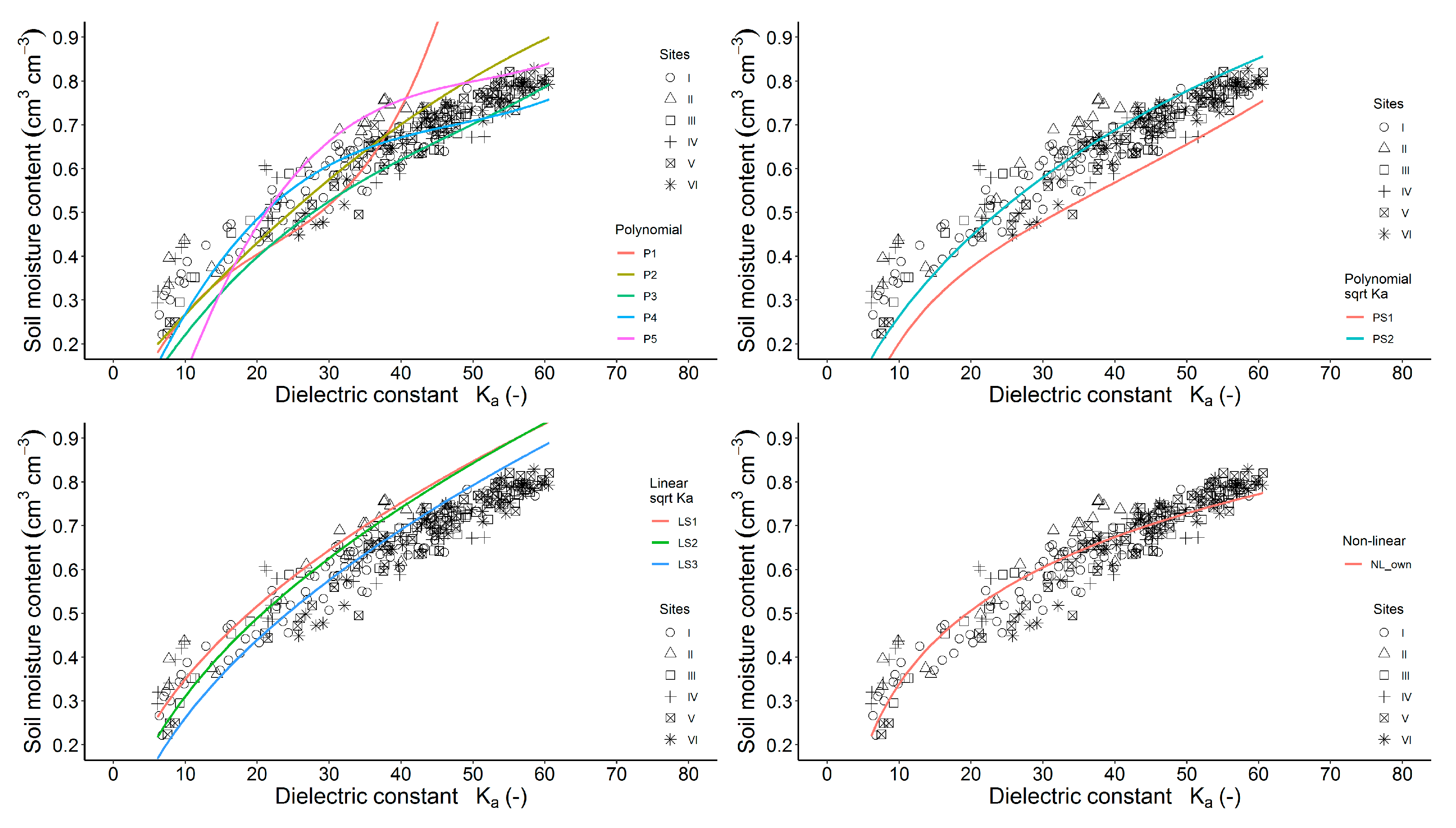
The relationship between the measured soil moisture content and the dielectric constant in respect to the field site is presented in Figure 2. Data are illustrated together with the TDR calibration curves for peat soils available in the literature listed in

Table 4. Selected literature calibration models for time domain reflectometry (TDR) methods and root mean square error (RMSE) statistics with respect to all collected dataset, as well as for data of the “dry” and “wet” segment of the general broken-line model (GBLM).

NO	Calibration Models	Soil	θv Range	Ka Range	Independent Variable	Function	Root Mean Square Error RMSE (cm3 cm−3)
							Overall Range of Data	Segments of GBLM Model
								“dry”	“wet”
1	P1 [23]	O	0.03–0.55	~3–35	Ka	p	0.4262	0.0924	0.5015
2	P2 [29]	SM	0.20–0.90	~5–60	Ka	p	0.0704	0.0764	0.0678
3	P3 [30]	O	0.00–0.75	~1–60	Ka	p	0.0748	0.1097	0.0546
4	P4 [31]	SC	0.30–0.80	~10–65	Ka	p	0.0571	0.0797	0.0448
5	P5 [32]	B	0.60–0.90	~29–75	Ka	p	0.1130	0.1672	0.0815
6	PS1[33]	SM	0.00–0.98	~3–75	sqrt (Ka)	p	0.1090	0.1364	0.0957
7	PS2 [33]	SM	0.00–0.98	~3–75	sqrt (Ka)	p	0.0586	0.0789	0.0480
8	LS1 [81]	O	0.10–0.80	~2–40	sqrt (Ka)	l	0.0958	0.0666	0.1053
9	LS2 [82]	Fo	0.00–0.70	~1–40	sqrt (Ka)	l	0.0908	0.0643	0.0996
10	LS3 [83]	SM	0.00–0.95	~2–73	sqrt (Ka)	l	0.0653	0.0801	0.0582
11	NL_own *	Mu	0.22–0.81	6–61	ln(Ka)	nl	0.0452	0.0586	0.0385
12	GBLM *	Mu	0.22–0.81	6–61	Ka	ls	0.0405	0.0508	0.0356

θ_v—volumetric soil moisture content (cm³ cm⁻³); K_a—dielectric constant (-); p—polynomial, l—linear; nl—nonlinear; ls—segmented linear; *—this study; O-organic soils, SC—Sphagnum, Carex peat SM-Sphagnum moss, B—blanket peat; Fo—forest soils, Mu—muck soils.

. A simple graphical inspection of the presented features indicates that any of the applied calibration equations do not fit the whole range of our dataset. The best prediction of the TDR soil moisture content for moorsh soil from the Biebrza River Valley can be approximated using equations P4 and PS2 [22].

The RMSE for these models was nearly 0.06 cm³ cm⁻³. Despite the reasonably good results of the RMSE statistic, the mentioned equations gave a satisfactory prediction of soil moisture content at different ranges of dielectric constant changes. The most appropriate literature model P4 enabled a reasonably good approximation of the soil moisture content in the range of dielectric constant between 10 and 20. The highest overestimation of soil moisture content (of about 0.15 cm³ cm⁻³) occurred when the dielectric constant was equal to 30. Figure 2 also shows the measured data of the soil moisture content and the dielectric constant and their fitting using the logarithmic model (NL_own) The following form of equation was obtained:

$${\mathsf{\theta }}_{\mathrm{v}}=0.2417·\ln \left({\mathrm{K}}_{\mathrm{a}}\right)-0.2173.$$

(4)

The calculated RMSE value was essentially lower (0.0452 cm³ cm⁻³) in comparison to the P4 and PS2 models. However, Equation (4) overestimated the moisture content by as much as 0.15 cm³ cm⁻³ in the middle range of the dielectric constant changes.

3.3. General and Site-Specific Relationships between Dielectric Constant and Soil Moisture Content

Based on the graphical inspection and simple statistical analysis, we decided to select the continuous broken-line model as an approximation to describe the non-linear relationship between soil moisture content and dielectric constant of the mucky soil (for all measured data of θ_v and K_a). For this purpose, the segmented linear regression was applied and the model parameters (Equations (1) and (3)) were estimated iteratively [67]. The results of the statistical computation indicated that the established continuous general broken-line model (GBLM) included one threshold parameter (Ψ), and can be written as:

$${\mathsf{\theta }}_{\mathrm{v}}=0.2335+0.01178·{\mathrm{K}}_{\mathrm{a}}{\mathrm{for}\mathrm{K}}_{\mathrm{a}}\le \mathsf{\psi },$$

(5)

$${\mathsf{\theta }}_{\mathrm{v}}=0.2335+0.01178·{\mathrm{K}}_{\mathrm{a}}-0.0046·\left({\mathrm{K}}_{\mathrm{a}}-\mathsf{\psi }\right){\mathrm{for}\mathrm{K}}_{\mathrm{a}}>\mathsf{\psi }.$$

(6)

After rearrangement the Equation (6) can be written in its final form as follows:

$${\mathsf{\theta }}_{\mathrm{v}}=0.2335+0.01178·\mathsf{\psi }+0.007179·\left({\mathrm{K}}_{\mathrm{a}}-\mathsf{\psi }\right){\mathrm{for}\mathrm{K}}_{\mathrm{a}}>\mathsf{\psi }.$$

(7)

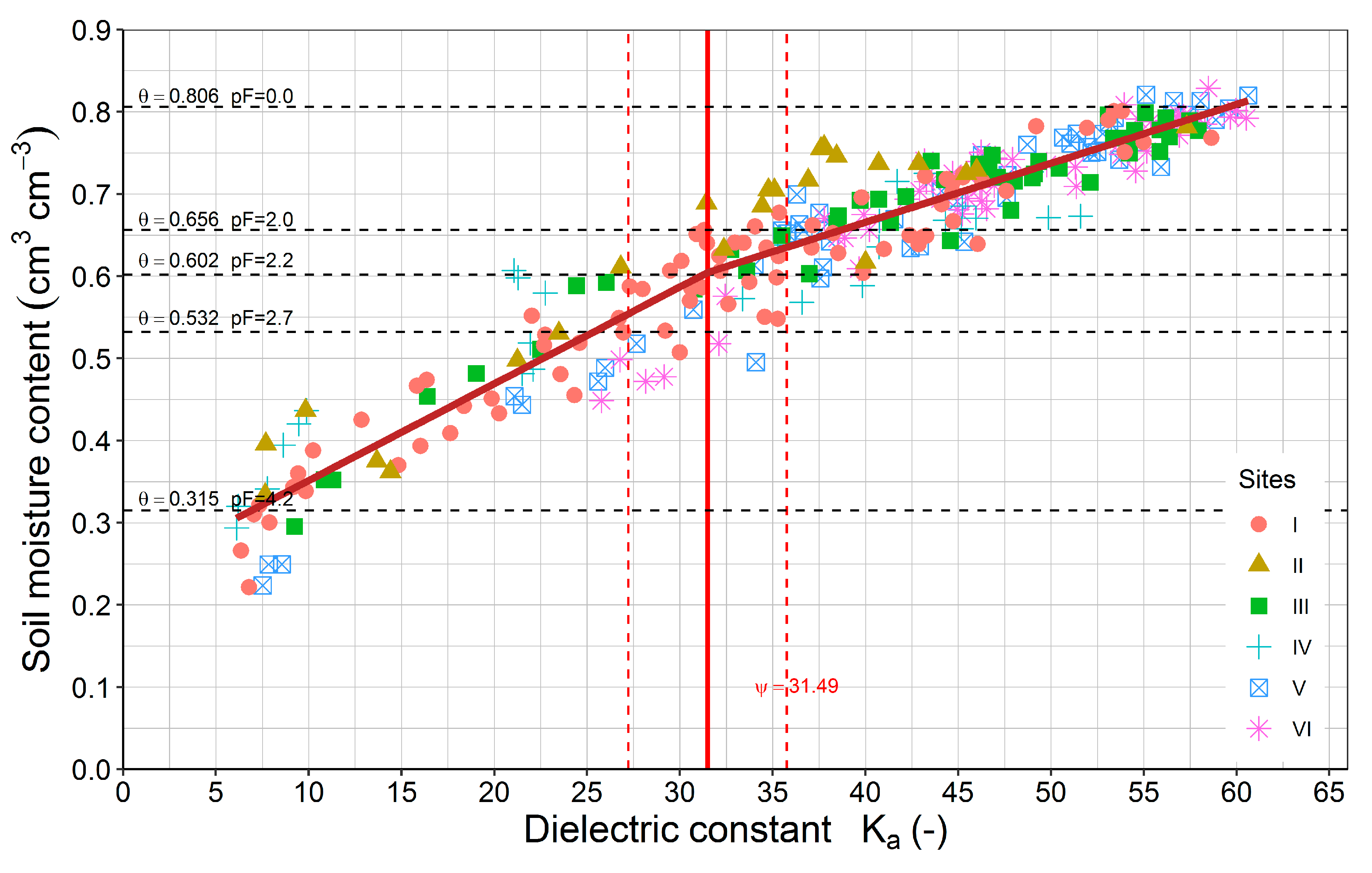
The break-point (Ψ) for the analyzed dataset was determined for K_a equal to 31.49 (Figure 3). The 95% confidence interval for this parameter was wide and ranged from 27.22 to 35.76 (Figure 3). Residuals from the model (Equations (5) and (6), or (5) and (7)) were normally distributed around the average which was confirmed by the Shapiro–Wilk testing statistic (W = 0.9919) and the p-value (0.1302). The RMSE value for the GBLM equations equals to 0.0405 cm³ cm⁻³ and is essentially lower than the estimates determined for the equations indicated in Table 4. This type of broken-line relationship is often used to assess the threshold value where the effect of the covariate changes. In the fields of hydrology and soil hydrology, the piecewise linear regressions (PLR) and the determined threshold values are used to explain the influence of the vegetation cover fraction on the reduction of runoff [84] and the erodibility coefficient [85]. In the water study, the two-segmented broken-line equation is applied for predicting water electrical conductivity using a portable X-ray fluorescence meter [86]. The meaning of a break-point in this study of the TDR calibration curve can be explained as the point depending on the soil water retention characteristic (horizontal lines on Figure 4). The threshold value (Ψ) with the confidence interval in general was included between horizontal lines which indicated the moisture contents at matric potential between pF values from 2.0 to 2.7. The average moisture content at break point (θ_ψ = 0.6044 cm³ cm⁻³) was approximately equal to soil moisture content at pF = 2.2 (θ_v = 0.6020 cm³ cm⁻³). The validity of the threshold value can be explained by bulk density changes (Figure 4).

The soil bulk density of the two segments was statistically different. For the “wet” range (segment wet above the threshold Ψ), the average bulk density was equal to 0.31 g cm⁻³, whereas at the “dry” range (segment dry) its estimates are equal to 0.33 g cm⁻³. It can be concluded that below the breakpoint of the θ_v(K_a) characteristic, the significant increase of bulk density indicates the essential soil volume changes. The field study conducted for similar soils confirmed that, apart from the soil moisture contents changes [87], the soil bulk density also changes in space and time [40].

Despite improvements in the GBLM model in comparison to the literature equations, the bias of the calibration equation depends on site-specific data measurements of θ_v(K_a). The segmented model gave a weak prediction of the soil moisture content for site II (bias equal to approximately 0.044 cm³ cm⁻³) as well as in the dry range of the soil moisture content in sites VI, V and IV.

The analysis of the GBLM model limitations forced us to develop the site-specific broken-line model (SSBLM). For this purpose, the linear regression lines were fitted for the analyzed sites in respect to data below and above the threshold value (Figure 3). The obtained slopes (β₁, β₁ + β₂) and intercepts (β₀) enabled the calculation of the breakpoint value separately for the soil from the specific sites. The parameters of the SSBLM models are summarized in

Table 5. Site-specific broken-line model parameters (SSBLM) for the TDR method.

Sites	β0	β1	β1 + β2	Ψ	θΨ
	(cm3 cm−3)	(cm3 cm−3)	(cm3 cm−3)	(-)	(cm3 cm−3)
I	0.2157	0.0125	0.00800	27.42	0.5585
II	0.2456	0.0129	0.00380	35.25	0.7003
III	0.1941	0.0144	0.00660	27.26	0.5866
IV	0.2587	0.0133	0.00640	18.29	0.5020
V	0.1330	0.0139	0.00810	34.98	0.6192
VI	0.0740	0.0147	0.00613	42.14	0.6935
Values of basic statistics
Mean 1	0.1869	0.01362	0.00651	30.89	0.6100
SD 2	0.0709	0.00086	0.00157	8.32	0.0776
CV 3	37.93	6.31	24.12	26.93	12.72

¹ mean—arithmetic average. ² SD—standard deviation. ³ CV—coefficient of variation (%).

.

Fitted lines below the threshold (“dry” range) were characterized by similar slope values (average value equal to 0.0136 and CV = 6.31%). In the “wet” range, slopes (β₁ + β₂) were generally flatter than in the “dry” range (β₁) and relatively more variable (CV = 24%) mainly because of the lowest slope of the θ_v(K_a) relationship for site II. Except for this site, the slope parameters in the “wet” range were also not essentially different. The Ψ parameter represents a wide range of changes in the dielectric constant (Table 5) which directly influences the really wide scatter of the soil moisture content (θ_Ψ) estimated at break point (Ψ). Despite the low CV value, the moisture content at the break points (θ_Ψ) ranged from 0.50 to 0.70 cm³ cm⁻³ which represents a relatively wide scatter for this type of soil. The comparison of θ_Ψ values with the range of moisture content of pF curves indicated that the threshold values were included in the range of the soil matric potential approximately between pF = 2.0 (site II) to pF = 2.5 (site IV).

Figure 5 shows the measured data of the soil moisture content and the dielectric constant for the specific sites and their fitting using the segmented model (SSBLM) and the logarithmic equations (NL type).

The SSBLM model developed separately for the soils from different sites indicates the reasonably good results of fitting in all ranges of the θ_v(K_a) relationship changes. The RMSE values were varied depending on the site data. For the calibration curves from sites III, V and VI, the values did not exceed 0.03 cm³ cm⁻³. The RMSE values for the rest of the developed SSBLM equations were slightly higher and varied from 0.036 cm³ cm⁻³ (site I) to 0.041 cm³ cm⁻³ (site IV). It should be stressed that logarithmic type models developed for specific site were less accurate and the RMSE value was generally higher (of about 0.005 to 0.012 cm³ cm⁻³) in comparison to the SSBLM models. The logarithmic models underestimated the soil moisture content by as much as 0.07 cm³ cm⁻³ in the wet range of calibration curve. From this reason for further analysis, we applied broken-line model parameters as an approximation of the non-linear relationship between K_a and θ_v.

3.4. Applicability Analysis of the Bio-Indices in Soil Moisture Prediction and Hydro-Physical Properties of Mucky Soils

Feasibility analysis of the calibration model development for the moorsh moisture content prediction as a function of dielectric constant with the participation of the covariates represented by bioindices is illustrated using the correlation coefficients (Figure 6).

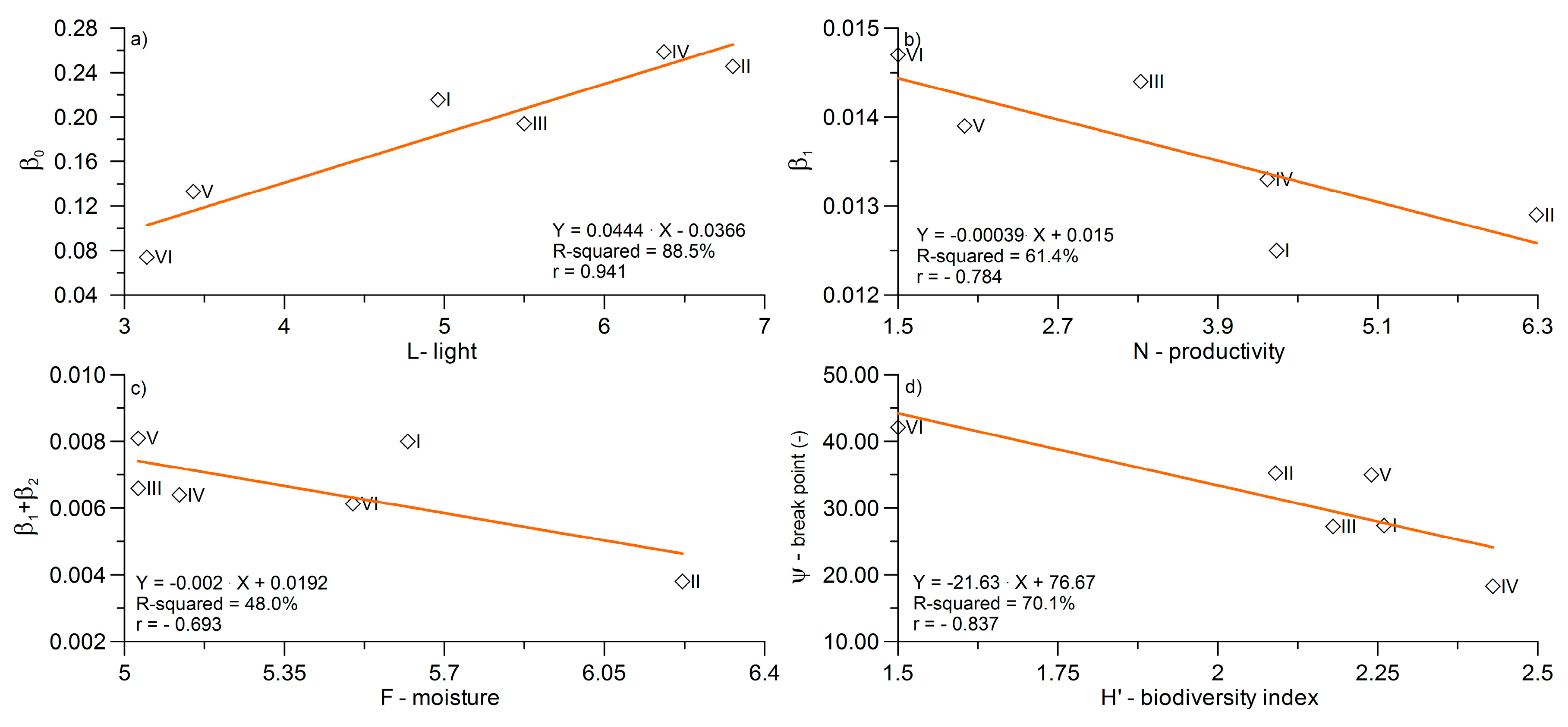
The broken-line model parameters (Table 5) were correlated with the bioindices (Table 3). The highest correlation coefficient has been noted between intercept (β₀) and indicator L of the Ellenberg scale. However, the β₀ also correlates with “productivity” of the ecosystem (N) as well as with the Shannon–Weiner index (H’). The slope in the “dry” range of the calibration curves (β₁) was strongly but negatively correlated with “productivity” of the ecosystem (N) determined on the basis of the plant cover as well as positively correlated with the ash content (AC) of the analyzed soils. Nevertheless, both of the explained covariates (AC and N) were moderately and negatively correlated, which can suggest that the increase of the AC amount in the soil causes reduction of the “productivity” of the analyzed ecosystems. The slope in the “wet” range of the calibration curves (β₁ + β₂) can be approximated using the soil moisture substrate indicator (F), which in the case of our studied sites describes fresh soil with moderate wetness [51]. Due to the low range of the F indicator changes and moderate variation of the β₁ + β₂ parameter, the prediction of the slope in the “wet” range of the calibration curve can be more complex than simple application of the linear relationship. The estimation of this parameter is especially important for the organic soils where soil moisture changes in the wet range strongly influence the soil degradation processes and physical soil properties. On the other hand, the β₁ + β₂ parameters were highly correlated with soil pF curve characteristics. From the data presented in Figure 6, it can be observed that these parameters were also negatively correlated with soil moisture contents measured at the predefined soil matric potentials ranging from pF = 1.5 to pF = 4.2. Moreover, it should be stressed that the moisture of the soil substrate (indicator F) was also highly correlated with the moisture content of the pF curves (Figure 6) which, in general, is in agreement with the statements made in [50]. Based on the correlation analysis, it can be noted that the slope in the “wet” range of the field calibration curves can be fairly well determined using the moisture indicator of the Ellenberg scale, or more precisely using the soil moisture content at pF = 2 as a soil type (site) specific predictor.

The broken-line model parameter Ψ was correlated with bioindicators of soil cover, physical soil properties and soil water retention characteristic. The highest r value was determined between Ψ and the Shannon–Weiner index. This could suggest that the variety of the plant species, which are typical for the site location, influences the slope separation point of the TDR calibration curves. This was especially visible in the case of two sites: VI and IV. In the former, the Ψ value was the highest and soil cover is mainly occupied by two plant species (Festuca rubra and Carex panicea) which affected the lowest value of the H’ index. On the other hand, at site IV the highest H’ value was observed (2.4) which indicates a condition of greater biodiversity (with a predominance of dicotyledonous plants), however, the Ψ value was the lowest (18.29). Although the Ψ value is was highly correlated with the Shannon–Weiner index, its value can also be carefully approximated by physical soil properties. Our data indicate that the increase of Ψ value was related to the increase of average soil porosity and soil moisture status at pF = 2.5 and 2.7. The Ψ value was also highly correlated with the ratio between L and F value suggesting an importance of light and moisture bioindicators in determination of the threshold value of the TDR calibration curve.

Figure 7a–d shows simple regression lines allowing prediction of the broken-line model parameters (Equations (1) and (3)) using bioindices (L, F, N, H’) determined on the basis of the measured plant species’ composition for the selected sites.

3.5. Calibration Model Development of Soil Moisture Content as a Function of Dielectric Constant and Botanical Indices of Soil Cover Using the Regression Tree Method

Based on the discussion presented in Section 3.4, we can state that the development of the general calibration curve for predicting moorsh moisture content using the TDR method for a specific site is very complex. We can predict each of the broken-line parameters one by one using simple linear equations plotted in Figure 7a–d. On the other hand, the simplification of the segmented line approach indicates that, for general purposes, both slopes (β₁, β₁ + β₂) can be averaged (Equations (5) and (7)), however, this requires finding out the threshold Ψ values. The quality of both attempts depends mainly on the prediction of the SSBLM parameters based on the bioindicators of the soil cover as the simplest explanatory variables. However, error in the estimation of the parameters affects the accuracy of the soil moisture prediction. Therefore, taking into account the temporal stability of the investigated ecosystems (supported by water supply and farmer practice), we developed a calibration equation which in one approach includes the relationship between soil moisture content and dielectric constant and the bioindicators’ influence. For this reason, we used the M5Rules algorithm belonging to regression tree methods (see description in Section 2.5).

Table 6. Summary of the cross-validation approach for establishing the site-specific model discontinuous (SSM-D) calibration model for the TDR method in mucky soils.

Model	Training Dataset	ntrain.	ntest.	Model Variables	RMSEtrain	RMSEcv
						SM	GBLM
SSM-D1	I, II, III, IV, V	227	51	Ka, F, L, N, H’	0.0351	0.0351	0.0406
SSM-D2	II, III, IV, V, VI	196	82	Ka, F, N, R, H’	0.0321	0.0326	0.0406
SSM-D3	I, III, IV, V, VI	256	22	Ka, F, N, L, R, H’	0.0318	0.0426	0.0411
SSM-D4	I, II, IV, V, VI	233	45	Ka, F, L, N	0.0362	0.0363	0.0406
SSM-D5	I, II, III, V, VI	251	27	Ka, F, L, N, H’	0.0301	0.0304	0.0409
SSM-D6	I, II, III, IV, VI	227	57	Ka, F, L, N, R, H’	0.0363	0.0368	0.0408

I, II, III, IV, V, VI—indicate the site data selected for model training; RMSE_train,cv (cm³ cm⁻³) for training model and for cross-validation scheme respectively; SM—set of model parameters including K_a, F, H’ and L variables.

summarizes the cross-validation scheme. In total we trained six models SSM-D1, …, SSM-D6. The results of the model selection approach indicate that, depending on training dataset, the SSM-D models included different explanatory variables for soil moisture prediction. The performance of the cross-validation split models is described by RMSE_train. The main independent variable in each training model, which binary split our dataset into two child sets, was dielectric constant (K_a). In the second stage of the cross-validation scheme we reduced the number of variables to the commonly appearing covariates in the training model stage. For this reason, different sets of explanatory variables were tested. Finally, we found the appropriate combination of the variables i.e., K_a, F, L and H’ (SM—set of model) in the model for which at each split of the data the RMSEcv values were close to the RMSE_train (Table 6). 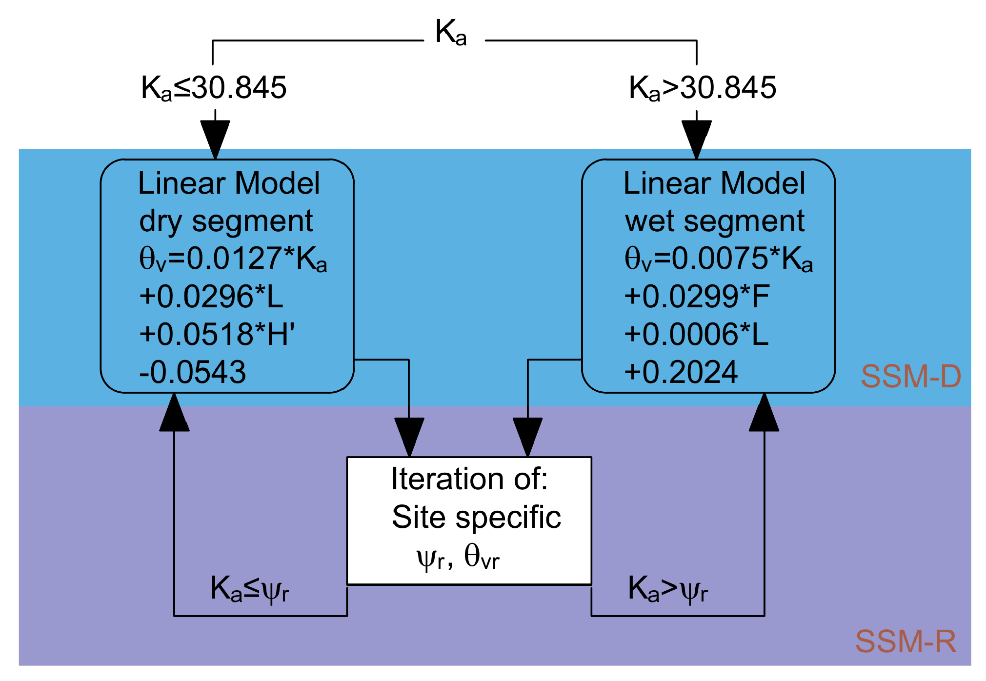Additionally, in Table 6 the RMSEcv values determined in cross-validation procedure performed for the GBLM model are also included. A last SSM-D model fitting was conducted using the mentioned combination of variables (SM) as single fit to all data. Fortunately, the resulted SSM-D model includes two nodes for which the linear regression models have been established (Figure 8).

This final fitting resulted in a two-slopes calibration model (SSM-D) split by the parent node (K_a = 30.845) similarly to the segmented regression model (Equations (5) and (7)). It should be stressed that the value of 30.845 is included in the confidence interval of the GBLM model. The slope of the line below the splitting point (dry range) was equal to 0.0127 (regression parameter at K_a variable) and was also comparable with its value determined using segmented regression (GBLM). The position of this line along the soil moisture content axis (the value of intercept) was improved by the H’ and L values (specific measures) of the site. Above the K_a = 30.845, the slope was equal to 0.0075 (nearly the same as in GBLM), however, the position of the line can be determined using covariates represented by F, L, bioindicators. However, it should be stressed that the influence of the L value was marginal for soil moisture prediction (wet range) which results from the regression coefficient at this variable.

Following the statements in [74], the regression tree indicated discontinuities occurring between adjacent leaves. In the post-processing procedure, we iteratively found out the threshold value ψ_r which enables establishing a continuous soil moisture content prediction model in the whole range of the dielectric constant changes (site-specific model with re-fitting of ψ_r value, SSM-R). This is especially important for monitoring of this feature. The uncertainty of this kind of the procedure was tested using the RMSE value as a criterion of losing quality in the model compared to the SSM-D model. The ψ_r values are in fact the re-established criterion of the splitting of the dataset which enables, again, application of the linear equations developed for both leaves (Figure 8).

The main conclusion from the modelling attempt is that the SSM-D model is structurally similar to the GBLM model (the splitting value K_a = 30.845 is similar to the ψ value of the GBLM model) and this results in discontinuities occurring between adjacent leaves. However, we propose to use the SSM-D model in the case when the TDR user does not want to perform a refitting (SSM-R). In the SSM-R model approach, additionally in the post-processing procedure, the threshold value in the form of ψ_r parameter is obtained. In this sense, the SSM-R model is the smoothed form of the SSM-D model and can be treated as a site-specific model similar to SSBLM. The inconveniences of the modelling approach as well as the importance of threshold value in mucky soils should be further investigated.

Table 7. Values of RMSE for the different types of TDR calibration models established in this study.

Sites	RMSE 1 for Different Calibration Models
	GBLM	SSBLM	SSM-D	SSM-R
overall	0.0405	0.0318	0.0351	0.0351
I	0.0361	0.0359	0.0370	0.0370
II	0.0623	0.0386	0.0489	0.0489
III	0.0264	0.0231	0.0270	0.0263
IV	0.0559	0.0410	0.0450	0.0450
V	0.0405	0.0300	0.0322	0.0318
VI	0.0349	0.0226	0.0273	0.0312

¹ RMSE—root mean square error (cm³ cm⁻³).

presents the RMSE value estimation according to the different calibration models for the TDR method. The results of the data presented in the table showed that the RMSE values for the proposed model (SSM-R) produce nearly the same error estimators as the SSM-D algorithm.

Based on this observation, we can state that the model, which is graphically presented in Figure 8, can be used for continuous prediction of moorsh soil moisture content based on dielectric constant measurements and complex information about bioindices. The form of the proposed model is generally in agreement with the main results of this study which showed the possibility to establish a two-segmented broken-line calibration model (GBLM, Equations (5) and (7)) for the TDR method.

4. Conclusions

Monitoring of soil moisture content in peat soil is a crucial issue which enables study processes related to peat soil degradation, particularly in the vadose zone. The presented study indicated that simple regression models which relate the soil dielectric constant with moisture content did not properly address determination of soil moisture content in degraded peatlands in field conditions. This was especially apparent in the intermediate range of dielectric constant changes (from approximately 20 to 40), where the best existing empirical models presented in the literature overestimated the moisture content by as much as 0.15 cm³ cm⁻³. The main expectation from TDR users is to be able to obtain relatively accurate moisture content determination in field conditions. The results of our investigations showed that the proposed calibration curve (GBLM) composed of two segments meets those requirements with the acceptable error of soil moisture determination in field conditions (RMSE = 0.04 cm³ cm⁻³). Despite the relatively good approximation of moisture content by the broken-line models (GBLM, SSBLM) developed during this study, these are only empirical equations, which should be subject to an interpretation derived from further investigation of the segmented line parameters. It is important to stress that in the case of the GBLM model, the existence of the two independent slopes separated by the threshold value ψ has been proved empirically by the statistically significant difference in soil bulk densities in both ranges of dielectric constant changes. We propose that further investigation should be focused on the assessment of the influence of soil air content on the slope of calibration equation in the dry range and assessment of the physical meaning of the threshold value ψ.

The conducted research also proved that, in site-specific calibration equations (SSBLM), the broken-line model parameters, in general, are correlated with the following bioindices: L, F, R, N values and biodiversity index (H’). This means that EIV and H’ indicators can be useful in the assessment of soil moisture content in degraded peatlands using the TDR technique. It should be stressed that an increase of slope value (β₁ + β₂) in the “wet” range of calibration equation was also correlated with a decrease of moisture content at pressure head corresponding to pF = 2. This tendency was also observed in the correlation between the F (substrate moisture) indicator and β₁ + β₂ slope. Moreover, it can be concluded that the F classifier of the habitats determined only on the basis of plant species’ composition is also highly correlated with the soil water retention characteristic at the investigated sites. Therefore, the performed research confirmed that the plant cover of the habitat depends on the water-related properties of the soil peatlands.

The analysis of the linear equations included in the SSM-D and SSM-R models indicates that the soil moisture content, aside from dielectric constant, was also dependent on the biodiversity index (H’) and light intensity (L) in the “dry” range of calibration curves. In the “wet” range of the calibration curve, the proposed model contains, apart from the variable (K_a), covariates represented by the following parameters: Substrate moisture (F), and light intensity (L).

The results of our study showed that bioindices, as well as their basic application, can also help in the identification of the specific soil condition which can improve our empirical knowledge of soil moisture regimes. Therefore, we hope the quantification of the EIV and H’ values of degraded peatlands as simply measured categorical variables will enable a TDR user to make decisions on what type of calibration equation can be selected for soil moisture monitoring in this type of ecosystem.

References

1. Vereecken, H.; Huisman, J.-A.; Franssen, H.H.; Brüggemann, N.; Bogena, H.R.; Kollet, S.; Javaux, M.; van der Kruk, J.; Vanderborght, J. Soil hydrology: Recent methodological advances, challenges, and perspectives. Water Resour. Res. 2015, 51, 2616–2633. [Google Scholar] [CrossRef] [Green Version]
2. Katul, G.G.; Oren, R.; Manzoni, S.; Higgins, C.; Parlange, M.B. Evapotranspiration: A process driving mass transport and energy exchange in the soil-plant-atmosphere-climate system. Rev. Geophys. 2012, 50. [Google Scholar] [CrossRef] [Green Version]
3. Holden, J.; West, L.J.; Howard, A.J.; Maxfield, E.; Panter, I.; Oxley, J. Hydrological controls of in situ preservation of waterlogged archaeological deposits. Earth Sci. Rev. 2006, 78, 59–83. [Google Scholar] [CrossRef] [Green Version]
4. Laiho, R. Decomposition in peatlands: Reconciling seemingly contrasting results on the impacts of lowered water levels. Soil Biol. Biochem. 2006, 38, 2011–2024. [Google Scholar] [CrossRef]
5. Gebhardt, S.; Fleige, H.; Horn, R. Shrinkage processes of a drained riparian peatland with subsidence morphology. J. Soils Sediments 2010, 10, 484–493. [Google Scholar] [CrossRef]
6. Strack, M. Peatlands and Climate Change; Strack, M., Ed.; IPS (International Peat Society): Helsinki, Finland, 2008; ISBN 952-99401-1-4. [Google Scholar]
7. Joosten, H.; Tapio-Biström, M.-L.; Tol, S. Peatlands: Guidance for Climate Change Mitigation through Conservation, Rehabilitation and Sustainable Use, 2nd ed.; Mitigation of Climate Change in Agriculture Series; Food and Agriculture Organization of the United Nations/Wetlands International: Rome, Italy, 2012; ISBN 978-92-5-107302-5. [Google Scholar]
8. Tanneberger, F.; Moen, A.; Joosten, H.; Nilsen, N. The peatland map of Europe. Mires Peat 2017, 19, 1–17. [Google Scholar]
9. Holden, J.; Chapman, P.J.; Labadz, J.C. Artificial drainage of peatlands: Hydrological and hydrochemical process and wetland restoration. Prog. Phys. Geogr. 2004, 28, 95–123. [Google Scholar] [CrossRef]
10. Joosten, H.; Clarke, D. Wise Use of Mires and Peatlands; International Mire Conservation Group/International Peat Society: Helsinki, Finland, 2002; ISBN 951-97744-8-3. [Google Scholar]
11. Okruszko, H.; Ilnicki, P. The moorsh horizons as quality indicators of reclaimed organic soils. In Organic Soils and Peat Materials for Sustainable Agriculture; Parent, L.E., Ilnicki, P., Eds.; CRC Press: Boca Raton, FL, USA, 2003; pp. 1–14. [Google Scholar]
12. Eswaran, H.; Reich, P.F.; Kimble, J.M.; Beinroth, F.H.; Padmanabhan, E.; Moncharoen, P. Global carbon stocks. In Global Climate Change and Pedogenic Carbonates; Lal, R., Kimble, J.M., Eswaran, H., Stewart, B.A., Eds.; CRC/Lewis: Boca Raton, FL, USA, 2000; pp. 15–25. [Google Scholar]
13. Kirschbaum, M.U. The temperature dependence of soil organic matter decomposition, and the effect of global warming on soil organic C storage. Soil Biol. Biochem. 1995, 27, 753–760. [Google Scholar] [CrossRef]
14. Wei, H.; Guenet, B.; Vicca, S.; Nunan, N.; AbdElgawad, H.; Pouteau, V.; Shen, W.; Janssens, I.A. Thermal acclimation of organic matter decomposition in an artificial forest soil is related to shifts in microbial community structure. Soil Biol. Biochem. 2014, 71, 1–12. [Google Scholar] [CrossRef]
15. Oleszczuk, R.; Regina, K.; Szajdak, L.; Höper, H.; Maryganova, V. Impacts of agricultural utilization of peat soils on the greenhouse gas balance. In Peatlands and Climate Change; Strack, M., Ed.; International Peat Society: Helsinki, Finland, 2008; pp. 70–97. ISBN 978-952-99401-1-0. [Google Scholar]
16. Mundel, G. Untersuchungen zur Torfmineralisation in Niedermooren. Arch. Acker-Pflanzenbau. Bodenkd. 1976, 20, 669–679. [Google Scholar]
17. Szanser, M. CO2 diffusion from peat-muck soils. I. Dependence of diffusion on temperature, moisture content and origin of soil. Pol. Ecol. Stud. 1991, 17, 85–99. [Google Scholar]
18. Mäkiranta, P.; Laiho, R.; Fritze, H.; Hytönen, J.; Laine, J.; Minkkinen, K. Indirect regulation of heterotrophic peat soil respiration by water level via microbial community structure and temperature sensitivity. Soil Biol. Biochem. 2009, 41, 695–703. [Google Scholar] [CrossRef]
19. Wessolek, G.; Schwärzel, K.; Renger, M.; Sauerbrey, R.; Siewert, C. Soil hydrology and CO2 release of peat soils. J. Plant Nutr. Soil Sci. 2002, 165, 494–500. [Google Scholar] [CrossRef]
20. Kluge, B.; Wessolek, G.; Facklam, M.; Lorenz, M.; Schwärzel, K. Long-term carbon loss and CO2-C release of drained peatland soils in northeast Germany. Eur. J. Soil Sci. 2008, 59, 1076–1086. [Google Scholar] [CrossRef]
21. Tiemeyer, B.; Borraz, E.A.; Augustin, J.; Bechtold, M.; Beetz, S.; Beyer, C.; Drösler, M.; Ebli, M.; Eickenscheidt, T.; Fiedler, S.; et al. High emissions of greenhouse gases from grasslands on peat and other organic soils. Glob. Chang. Biol. 2016, 22, 4134–4149. [Google Scholar] [CrossRef] [PubMed]
22. Bircher, S.; Andreasen, M.; Vuollet, J.; Vehviläinen, J.; Rautiainen, K.; Jonard, F.; Weihermüller, L.; Zakharova, E.; Wigneron, J.-P.; Kerr, Y.H. Soil moisture sensor calibration for organic soil surface layers. Geosci. Instrum. Method. Data Syst. 2016, 5, 109–125. [Google Scholar] [CrossRef] [Green Version]
23. Topp, G.C.; Davis, J.L.; Annan, A.P. Electromagnetic determination of soil water content: Measurements in coaxial transmission lines. Water Resour. Res. 1980, 16, 574–582. [Google Scholar] [CrossRef]
24. Jones, S.B.; Or, D. Modeled effects on permittivity measurements of water content in high surface area porous media. Phys. B Condens. Matter 2003, 338, 284–290. [Google Scholar] [CrossRef]
25. Nagare, R.; Schincariol, R.; Quinton, W.; Hayashi, M. Laboratory calibration of time domain reflectometry to determine moisture content in undisturbed peat samples. Eur. J. Soil Sci. 2011, 62, 505–515. [Google Scholar] [CrossRef]
26. Dettmann, U.; Bechtold, M. Evaluating commercial moisture probes in reference solutions covering mineral to peat soil conditions. Vadose Zone J. 2018, 17. [Google Scholar] [CrossRef]
27. Weitz, A.M.; Grauel, W.; Keller, M.; Veldkamp, E. Calibration of time domain reflectometry technique using undisturbed soil samples from humid tropical soils of volcanic origin. Water Resour. Res. 1997, 33, 1241–1249. [Google Scholar] [CrossRef] [Green Version]
28. Sakaki, T.; Limsuwat, A.; Smits, K.M.; Illangasekare, T.H. Empirical two-point α-mixing model for calibrating the ECH2O EC-5 soil moisture sensor in sands. Water Resour. Res. 2008, 44. [Google Scholar] [CrossRef]
29. Pepin, S.; Plamondon, A.P.; Stein, J. Peat water content measurement using time domain reflectometry. Can. J. For. Res. 1992, 22, 534–540. [Google Scholar] [CrossRef]
30. Roth, C.H.; Malicki, M.A.; Plagge, R. Empirical evaluation of the relationship between soil dielectric constant and volumetric water content as the basis for calibrating soil moisture measurements by TDR. J. Soil Sci. 1992, 43, 1–13. [Google Scholar] [CrossRef]
31. Myllys, M.; Simojoki, A. Calibration of time domain reflectometry (TDR) for soil moisture measurements in cultivated peat soils. Suo 1996, 47, 1–6. [Google Scholar]
32. Beckwith, C.W.; Baird, A.J. Effect of biogenic gas bubbles on water flow through poorly decomposed blanket peat. Water Resour. Res. 2001, 37, 551–558. [Google Scholar] [CrossRef] [Green Version]
33. Yoshikawa, K.; Overduin, P.P.; Harden, J.W. Moisture content measurements of moss (Sphagnum spp.) using commercial sensors. Permafrost Periglac. Process. 2004, 15, 309–318. [Google Scholar] [CrossRef]
34. Kujala, K.; Seppälä, M.; Holappa, T. Physical properties of peat and palsa formation. Cold Reg. Sci. Technol. 2008, 52, 408–414. [Google Scholar] [CrossRef]
35. Jones, S.B.; Wraith, J.M.; Or, D. Time domain reflectometry measurement principles and applications. Hydrol. Process. 2002, 16, 141–153. [Google Scholar] [CrossRef]
36. Shibchurn, A.; Van Geel, P.J.; Kennedy, P.L. Impact of density on the hydraulic properties of peat and the time domain reflectometry (TDR) moisture calibration curve. Can. Geotech. J. 2005, 42, 279–286. [Google Scholar] [CrossRef]
37. Malicki, M.; Plagge, R.; Roth, C. Improving the calibration of dielectric TDR soil moisture determination taking into account the solid soil. Eur. J. Soil Sci. 1996, 47, 357–366. [Google Scholar] [CrossRef]
38. Oleszczuk, R.; Gnatowski, T.; Brandyk, T.; Szatylowicz, J. Calibration of TDR for moisture content monitoring in moorsh layers. In Wetlands Monitoring, Modelling and Management; Okruszko, T., Maltby, E., Szatylowicz, J., Swiatek, D., Kotowski, W., Eds.; Taylor & Francis Group: London, UK, 2007; pp. 121–124. ISBN 978-0-415-40820-2. [Google Scholar]
39. Schlotzhauer, S.M.; Price, J.S. Soil water flow dynamics in a managed cutover peat field, Quebec: Field and laboratory investigations. Water Resour. Res. 1999, 35, 3675–3683. [Google Scholar] [CrossRef] [Green Version]
40. Szatylowicz, J.; Gnatowski, T.; Szejba, D.; Oleszczuk, R.; Brandyk, T.; Kechavarzi, C. Moisture content variability in drained fen soil. In Wetlands Monitoring, Modelling and Management; Okruszko, T., Maltby, E., Szatyłowicz, J., Swiatek, D., Kotowski, W., Eds.; Taylor & Francis Group: London, UK, 2007; pp. 113–120. ISBN 978-0-415-40820-2. [Google Scholar]
41. Altdorff, D.; Bechtold, M.; van der Kruk, J.; Vereecken, H.; Huisman, J.A. Mapping peat layer properties with multi-coil offset electromagnetic induction and laser scanning elevation data. Geoderma 2016, 261, 178–189. [Google Scholar] [CrossRef]
42. Hewelke, E.; Szatyłowicz, J.; Gnatowski, T.; Oleszczuk, R. Effects of soil water repellency on moisture patterns in a degraded sapric histosol. Land Degrad. Dev. 2016, 27, 955–964. [Google Scholar] [CrossRef]
43. Könönen, M.; Jauhiainen, J.; Laiho, R.; Kusin, K.; Vasander, H. Physical and chemical properties of tropical peat under stabilised land uses. Mires Peat 2015, 16, 1–13. [Google Scholar]
44. Knoepp, J.D.; Coleman, D.C.; Crossley, D., Jr.; Clark, J.S. Biological indices of soil quality: An ecosystem case study of their use. For. Ecol. Manag. 2000, 138, 357–368. [Google Scholar] [CrossRef]
45. Ellenberg, H.; Weber, H.E.; Dull, R.; Wirth, V.; Werner, W.; Paulissen, D. Zeigerwerte von Pflanzen in Mitteleuropa. Scr. Geobot. 1991, 18, 1–258. [Google Scholar]
46. Pinckney, J.L.; Quigg, A.S.; Roelke, D.L. Interannual and seasonal patterns of estuarine phytoplankton diversity in Galveston Bay, Texas, USA. Estuaries Coast. 2017, 40, 310–316. [Google Scholar] [CrossRef]
47. Paerl, H.W.; Valdes, L.M.; Pinckney, J.L.; Piehler, M.F.; Dyble, J.; Moisander, P.H. Phytoplankton photopigments as indicators of estuarine and coastal eutrophication. AIBS Bull. 2003, 53, 953–964. [Google Scholar] [CrossRef]
48. Zettler, M.L.; Schiedek, D.; Bobertz, B. Benthic biodiversity indices versus salinity gradient in the southern Baltic Sea. Mar. Poll. Bull. 2007, 55, 258–270. [Google Scholar] [CrossRef]
49. Chytrỳ, M.; Hejcman, M.; Hennekens, S.M.; Schellberg, J. Changes in vegetation types and Ellenberg indicator values after 65 years of fertilizer application in the Rengen Grassland Experiment, Germany. Appl. Veg. Sci. 2009, 12, 167–176. [Google Scholar] [CrossRef] [Green Version]
50. Schaffers, A.P.; Sýkora, K.V. Reliability of Ellenberg indicator values for moisture, nitrogen and soil reaction: A comparison with field measurements. J. Veg. Sci. 2000, 11, 225–244. [Google Scholar] [CrossRef]
51. Simmel, J.; Bässler, C.; Poschlod, P. Ellenberg indicator values for macromycetes–a methodological approach and first applications. Fungal Ecol. 2017, 27, 202–212. [Google Scholar] [CrossRef]
52. Klaus, V.H.; Kleinebecker, T.; Boch, S.; Müller, J.; Socher, S.A.; Prati, D.; Fischer, M.; Hölzel, N. NIRS meets Ellenberg’s indicator values: Prediction of moisture and nitrogen values of agricultural grassland vegetation by means of near-infrared spectral characteristics. Ecol. Indic. 2012, 14, 82–86. [Google Scholar] [CrossRef]
53. Diekmann, M. Species indicator values as an important tool in applied plant ecology—A review. Basic Appl. Ecol. 2003, 4, 493–506. [Google Scholar] [CrossRef]
54. Kollmann, J.; Fischer, A. Vegetation as indicator for habitat quality. Basic Appl. Ecol. 2003, 4, 489–491. [Google Scholar] [CrossRef]
55. Szuniewicz, J.; Chrzanowski, S. Przeobrażanie się i spłycanie odwodnionych gleb torfowych na przykladzie torfowiska Kuwasy. Materiały Seminaryjne. Instytut Melioracji Użytków Zielonych 1995, 34, 241–246. [Google Scholar]
56. Agriculture Organization for the United Nations. World Reference Base for Soil Resources; World Soil Resources Report; FAO: Rome, Italy, 2006. [Google Scholar]
57. Charzyński, P. Testing WRB on Polish Soils; Association of Polish Adult Education: Toruń, Poland, 2006. [Google Scholar]
58. Kellogg, C.E. Soil Survey Division Staff Soil Survey Manual; United States Department of Agriculture: Washington, DC, USA, 1993. [Google Scholar]
59. Skierucha, W.; Wilczek, A.; Szypłowska, A.; Sławiński, C.; Lamorski, K. A TDR-based soil moisture monitoring system with simultaneous measurement of soil temperature and electrical conductivity. Sensors 2012, 12, 13545–13566. [Google Scholar] [CrossRef]
60. Okruszko, H. Określanie ciężaru właściwego gleb hydrogenicznych na podstawie zawartości w nich części mineralnych. Wiad. IMUZ 1971, 10, 37–54. [Google Scholar]
61. Brandyk, T.; Szatylowicz, J.; Oleszczuk, R.; Gnatowski, T. Water-related physical attributes of organic soils. In Organic Soils and Peat Materials for Sustainable Agriculture; Parent, L.E., Ilnicki, P., Eds.; CRC Press: Boca Raton, FL, USA, 2002; pp. 33–66. [Google Scholar]
62. Klute, A. Water retention: Laboratory methods. In Methods of Soil Analysis. Part 1, Physical and Mineralogical Methods; ASA/SSSA: Madison, WI, USA, 1986; pp. 635–662. [Google Scholar]
63. Krebs, C.J. Ecological Methodology, 2nd ed.; Harper & Row: New York, NY, USA, 1989. [Google Scholar]
64. Colwell, R.K. Biodiversity: Concepts, patterns, and measurement. In The Princeton Guide to Ecology; Levin, S.A., Carpenter, S.R., Godfray, H.C., Kinzig, A.P., Loreau, M., Losos, J.B., Walker, B., Wilcove, D.S., Eds.; Princeton University Press: Princeton, NJ, USA, 2009; pp. 257–263. [Google Scholar]
65. Muggeo, V.M. Estimating regression models with unknown break-points. Stat. Med. 2003, 22, 3055–3071. [Google Scholar] [CrossRef]
66. Toms, J.D.; Lesperance, M.L. Piecewise regression: A tool for identifying ecological thresholds. Ecology 2003, 84, 2034–2041. [Google Scholar] [CrossRef]
67. Muggeo, V.M. Segmented: An R package to fit regression models with broken-line relationships. R News 2008, 8, 20–25. [Google Scholar]
68. Blanco, C.M.G.; Gomez, V.M.B.; Crespo, P.; Ließ, M. Spatial prediction of soil water retention in a Páramo landscape: Methodological insight into machine learning using random forest. Geoderma 2018, 316, 100–114. [Google Scholar] [CrossRef]
69. Hornik, K.; Buchta, C.; Zeileis, A. Open-source machine learning: R meets Weka. Comput. Stat. 2009, 24, 225–232. [Google Scholar] [CrossRef]
70. Quinlan, J.R. Learning with continuous classes. In Proceedings of the Australian Joint Conference on Artificial Intelligence, Hobart, Australia, 16–18 November 1992; Volume 92, pp. 343–348. [Google Scholar]
71. Frank, E.; Hall, M.; Holmes, G.; Kirkby, R.; Pfahringer, B.; Witten, I.H.; Trigg, L. Weka-a machine learning workbench for data mining. In Data Mining and Knowledge Discovery Handbook; Maimon, O., Rokach, L., Eds.; Springer US: Boston, MA, USA, 2010; pp. 1269–1277. ISBN 978-0-387-09822-7. [Google Scholar]
72. Yang, L.; Liu, S.; Tsoka, S.; Papageorgiou, L.G. Mathematical programming for piecewise linear regression analysis. Expert Syst. Appl. 2016, 44, 156–167. [Google Scholar] [CrossRef] [Green Version]
73. Torgo, L. Data Mining with R: Learning with Case Studies, 2nd ed.; Chapman and Hall/CRC: New York, NY, USA, 2016; ISBN 1-315-39909-1. [Google Scholar]
74. Holmes, G.; Hall, M.; Prank, E. Generating rule sets from model trees. In Advanced Topics in Artificial Intelligence; Springer: Sydney, Australia, 1999; pp. 1–12. [Google Scholar]
75. Roberts, D.R.; Bahn, V.; Ciuti, S.; Boyce, M.S.; Elith, J.; Guillera-Arroita, G.; Hauenstein, S.; Lahoz-Monfort, J.J.; Schröder, B.; Thuiller, W. Cross-validation strategies for data with temporal, spatial, hierarchical, or phylogenetic structure. Ecography 2017, 40, 913–929. [Google Scholar] [CrossRef] [Green Version]
76. Kechavarzi, C.; Dawson, Q.; Leeds-Harrison, P.B. Physical properties of low-lying agricultural peat soils in England. Geoderma 2010, 154, 196–202. [Google Scholar] [CrossRef]
77. Berglund, Ö.; Berglund, K.; Klemedtsson, L. A lysimeter study on the effect of temperature on CO2 emission from cultivated peat soils. Geoderma 2010, 154, 211–218. [Google Scholar] [CrossRef]
78. Kløve, B.; Sveistrup, T.; Hauge, A. Leaching of nutrients and emission of greenhouse gases from peatland cultivation at Bodin, Northern Norway. Geoderma 2010, 154, 219–232. [Google Scholar] [CrossRef]
79. Wallor, E.; Rosskopf, N.; Zeitz, J. Hydraulic properties of drained and cultivated fen soils part I-Horizon-based evaluation of van Genuchten parameters considering the state of moorsh-forming process. Geoderma 2018, 313, 69–81. [Google Scholar] [CrossRef]
80. Oleszczuk, R.; Szatyłowicz, J.; Brandyk, T.; Gnatowski, T. An analysis of the influence of shrinkage on water retention characteristics of fen peat-moorsh soil. Suo 2000, 51, 139–147. [Google Scholar]
81. Herkelrath, W.N.; Hamburg, S.P.; Murphy, F. Automatic, real-time monitoring of soil moisture in a remote field area with time domain reflectometry. Water Resour. Res. 1991, 27, 857–864. [Google Scholar] [CrossRef]
82. Schaap, M.G.; De Lange, L.; Heimovaara, T.J. TDR calibration of organic forest floor media. Soil Technol. 1997, 11, 205–217. [Google Scholar] [CrossRef]
83. Caron, J.; Rivière, L.-M.; Charpentier, S.; Renault, P.; Michel, J.-C. Using TDR to estimate hydraulic conductivity and air entry in growing media and sand. Soil Sci. Soc. Am. J. 2002, 66, 373–383. [Google Scholar] [CrossRef]
84. Roundy, B.A.; Farmer, M.; Olson, J.; Petersen, S.; Nelson, D.R.; Davis, J.; Vernon, J. Runoff and sediment response to tree control and seeding on a high soil erosion potential site in Utah: Evidence for reversal of an abiotic threshold. Ecohydrology 2017, 10, e1775. [Google Scholar] [CrossRef]
85. Al-Hamdan, O.Z.; Pierson, F.B.; Nearing, M.A.; Williams, C.J.; Hernandez, M.; Boll, J.; Nouwakpo, S.K.; Weltz, M.A.; Spaeth, K. Developing a parameterization approach for soil erodibility for the Rangeland Hydrology and Erosion Model (RHEM). Trans. ASABE 2017, 60, 85–94. [Google Scholar]
86. Pearson, D.; Chakraborty, S.; Duda, B.; Li, B.; Weindorf, D.C.; Deb, S.; Brevik, E.; Ray, D. Water analysis via portable X-ray fluorescence spectrometry. J. Hydrol. 2017, 544, 172–179. [Google Scholar] [CrossRef]
87. Hewelke, E.; Szatyłowicz, J.; Gnatowski, T.; Oleszczuk, R. Zmienność przestrzenna uwilgotnienia hydrofobowej gleby organicznej w warunkach przepływu preferencyjnego. Rocznik Ochrona Środowiska 2014, 16, 580–607. [Google Scholar]
Figure 1. Location of study sites (based on http://mapy.geoportal.gov.pl).
Water 10 01842 g001
Figure 2. Measured data of dielectric constant and soil moisture content for different sites together with own empirical relationship (NL_own) and relationships listed in Table 4.
Water 10 01842 g002
Figure 3. Field measurements and fitted GBLM for the relationship between soil moisture content and dielectric constant. The horizontal dotted black lines indicate the soil moisture content at predefined pressure head. The red vertical line indicates the average value of the breaking point (ψ = 31.49) whereas the red dotted vertical line is the 95% confidence interval.
Water 10 01842 g003
Figure 4. Boxplot of soil bulk density for “dry” and “wet” segments of the measured dataset (dotted line indicates overall average soil bulk density). The scattered point indicates the soil bulk density value with respect to sites. The dotted horizontal line indicates the overall soil bulk density average. The diamond symbol indicates the average soil bulk density for each segment of the dataset. The red dots indicate the outliers.
Water 10 01842 g004
Figure 5. Field measurements and fitted models of the relationship between the soil moisture content and dielectric constant for specific sites. (a) Site I; (b) site II; (c) site III; (d) site IV; (e) site V; (f) site VI.
Water 10 01842 g005
Figure 6. Correlation graph of the analyzed variables. Arrows in green and red indicate statistically significant positive and negative correlations. Dark yellow arrows indicate not statistically significant correlations. The labelled cells indicate statistically significant correlation between different types of variables regarding the state of the habitats, SSBLM and soil hydro-physical properties.
Water 10 01842 g006
Figure 7. Linear regression lines between parameters of the broken-line model and explanatory variables: (a) the Ellenberg index L - light vs. the intercept β0 of SSBLM; (b) the Ellenberg index N – productivity vs. the slope β1 of SSBLM; (c) the Ellenberg index F – moisture vs. the slope β1 + β2 of SSBLM; (d) the biodiversity index – H’ vs. the breakpoint (Ψ) of SSBLM.
Water 10 01842 g007
Figure 8. Diagram representing graphical explanation of the SSM-D and site-specific model with re-fitting of ψr value (SSM-R) models.
Water 10 01842 g008