Effectiveness of Contour Farming and Filter Strips on Ecosystem Services


1
Water Engineering, Institute of Water and Energy Sciences, Pan African University, 13000 Tlemcen, Algeria
2
Center for Middle Eastern Studies, Lund University, 22100 Lund, Sweden
3
Department of soil, water and environmental engineering Jomo Kenyatta University of Agriculture and Technology (JKUAT), 00200 Nairobi, Kenya
*
Author to whom correspondence should be addressed.
Water 2018, 10(10), 1312; https://doi.org/10.3390/w10101312
Submission received: 2 August 2018
/
Revised: 17 August 2018
/
Accepted: 18 September 2018
/
Published: 22 September 2018
(This article belongs to the Special Issue Hydroeconomic Analysis for Sustainable Water Management)
Abstract
:The failing ecosystem services in Thika-Chania catchment is manifested in the deterioration of water quality, sedimentation of reservoirs, and subsequent increase in water treatment costs due to high turbidity. The services can be restored by implementing relevant soil and water conservation practices to enhance flow regulation and control sediment yield. The impacts of contour farming and filter strips on water and sediment yield were evaluated using Soil Water and Assessment Tool (SWAT), Texas A&M University, USA. Sediment calibration and validation was achieved using data obtained from a bathymetric survey. Model parameters were adjusted to simulate the conservation impacts of contour farming and filter strips. Results indicated the average annual sediment yield as 22 t/ha at the outlet of the catchment and average annual surface runoff of 202 mm. The simulation results showed that filter strips of 5 m width would reduce the average annual sediment yield from the catchment by 54%. The efficacy of filter strips in reducing sediment yield was observed to increase with increasing filter width. Three-meter filter strips and contour farming reduced the average annual sediment yield at catchment outlet by 46% and 36%, respectively. It was concluded that the implementation of contour farming and filters strips reduced sediments by 63% from the base value. Water yield at the sub-basin level was only influenced by contour farming. The total water yield at the catchment outlet experienced no significant change.
1. Introduction
Human beings benefit from a wide range of ecosystem services provided by nature around the world, including fresh water, firewood, flood regulation, purification of water, and creation of an aesthetic ecosystem. These services, however, are affected by the unsustainable use of those ecosystems. About 50% of the arable land in the world has been affected by soil erosion, leading to deterioration of ecosystem services from which people derive their livelihoods [1]. Approximately 5 t/ha of productive soil is eroded for water resources annually in Africa [2]. When soil is transported in surface runoff it causes sedimentation of reservoirs, enhances algae growth in watercourses, and creates a risk of flooding in low-lying areas, besides deteriorating the quality of water.
Modeling water resources is considered one of the most important tools in assessing water resources issues at the catchment level [3,4,5,6], avoiding spreadsheet calculations to predict assumptions and factors [7,8]. Hydrology in a catchment is divided into two phases: the land phase and the routing phase [9]. Across the globe, studies have been conducted on ecosystem services, mainly focused on more than one service provided by the watersheds and catchment ecosystems. Most of the studies concentrate on economic valuation of the ecosystem services and studying their biophysical processes [10], such as one that assessed the provisioning and cultural ecosystem services in natural wetlands and rice fields in Kenya. The services evaluated include fiber, building materials, and foodstuffs that were quantified as biophysical quantities and monetary value. The provisioning services have declined in the past decades, while sustainable utilization of the systems is crucial in livelihood enhancement [10]. Contour farming is an agronomic conservation method whereby farming activities are done across a slope as opposed to up and down it [11]. The practice reduces soil erosion down the slope by creating crop row ridges that act as barriers to surface runoff, thus reducing flow velocity and enhancing infiltration in the small depressions formed. Contour cultivation has been adopted across the world as an effective way of controlling soil erosion and preventing sedimentation [12,13,14]. The main purpose of filter strips is to reduce the amount of suspended materials and sediments on runoff water [15]. Research has been conducted assessing the effectiveness of filter strips in reducing sedimentation and siltation in water bodies through modeling or the use of experimental plots [16,17,18,19,20]. Evaluation using experimental methods, however, takes a relatively long time as compared to simulation using models. SWAT estimates sediment deposition and the amount of sediment from a catchment as a function of water volume from the stream segment [17].
In Thika-Chania catchment, soil erosion and subsequent sedimentation of reservoirs have increased sedimentation and subsequent loss of water storage volume in downstream reservoirs [21,22,23]. Most of the inhabitants in the catchment derive their livelihoods from agriculture [17]. In a baseline survey carried out in the catchment, 77% of people said that erosion occurs on their farms and 54% of the inhabitants had less than 25% of their land under soil conservation methods [24]. Most people (53%) noted a declining vegetation cover on their land, while 79% observed a greater deterioration in water quality in rainy seasons compared to half a decade ago. This implies that soil erosion continues to increase as vegetation cover on the land decreases.
Previous studies have highlighted the need to implement soil and water conservation measures in the catchment [24,25]. However, before their implementation, the effectiveness of each conservation method needs to be established as the effectiveness of any management practice varies from one region to another and from one sub-catchment to another due to different land uses, slope, and climatic conditions. This research aims at evaluating the impacts of conservation measures on sediment and water yield, which are the regulating and provisioning services of the ecosystem, using a SWAT model.
2. Materials and Methods
2.1. Study Area
Thika-Chania catchment spans over four counties in Kenya and lies between latitude 36.58° and 37.58° E and 0.58° and 1.17° S. Hydrologically, the catchment is located in the Upper Tana Catchment and has a total area of 840 km2 (Figure 1). Thika and Chania rivers are the main drainage systems in the catchment. At the outlet of the catchment, the two rivers join and then drain into Masinga reservoir. Slopes in the study area vary from gently sloping to very steep with the predominant slopes in the range of 0–20%. This represents 70% of the total catchment area. The major land use is agriculture, which includes coffee, tea, and cultivation of horticultural crops. In the upper parts of the catchment is a forest cover that aids in filtration of water from the cultivated areas upstream. Distribution of rainfall is bimodal, with high peaks from March to May and short rains coming in October to December. Rainfall varies from 800 mm in low-altitude areas (1525 m a.s.l.) to 2200 mm in high-altitude areas of the catchment. The dominant soils in the catchment include mollic andosol and humic nitisols.
2.2. Data Acquisition, Calibration, and Validation of the SWAT Model
2.3. Model Setup
The land phase controls the amounts of sediments, water, pesticides, and nutrients that enter the main channel for every sub-basin. In SWAT model, the land phase is described by the following equation:
where:
- SWt: the final soil water content (mm),
- SW0: the initial water content in day i (mm),
- R: the amount of precipitation in day i (mm),
- Qs: the amount of surface runoff in day i (mm),
- Ea: the amount of evaporation in day i (mm),
- Wseep: the amount of water entering the vadose zone in day i (mm),
- Qqw: the amount of return flow in day i (mm).
Erosion calculation and sediment yield calculation in SWAT uses the Modified Universal Soil Loss Equation (MUSLE), which is a modified form of the USLE. MUSLE predicts sediment yield based on runoff factor, while USLE predicts sediment yield based on rainfall energy factor [28]. MUSLE therefore accounts for the antecedent soil moisture and estimates of sediment from a single storm can be determined.
where,
- Sed: Sediment yield from a given Hydrologic Response Unit HRU on storm event basis (t/ha),
- Q: Surface runoff volume (mm/ha),
- qp: Peak runoff (m3/s),
- K: Soil erodibility (Mg MJ−1 mm−1),
- C: Crop management factor (Dimensionless)
- P: Soil erosion control practice (Dimensionless)
- LS: Topographic factor (L: slope length, S: slope steepness) (Dimensionless),
- A: Hydrologic Response Unit (HRU) (ha),
- CFRG: Coarse fragment factor (Dimensionless).
The digital elevation model, soil map, and land use maps were projected to the same coordinate system. A user-defined critical source area of 1200 ha was adopted as the average sub-basin area fell within the recommended range of 2–5% of the total catchment area [29]. The projected land use map was uploaded into the model and reclassified to align with SWAT land-use types. In order to reclassify the land use type, a user look-up table was made to identify the SWAT land use codes that correspond to the land use map (Figure 2).
Key parameters lacking in the SOTER soil database are the saturated hydraulic conductivity and USLE soil erodibility factor (K) for each soil type and layer. The saturated hydraulic conductivity (KS) was estimated using the Jabro method [30], which was used by [22]:
Log (KS) = 9.56 − 0.81 log(% silt) − 1.09 log(% clay) − 4.64 (bulk density).
The structure of the soil is influenced by the percent clay, silt, or organic matter present. The information on the properties of these soils was found in the soil terrain database. From the analysis of different soils in the catchment area, it was noted that the texture of the soil influenced its saturated hydraulic conductivity. That is, the higher the percentage of silt and clay, the lower the saturated hydraulic conductivity.
The USLE erodibility factor was estimated using the method explained in [31].
The Hydrologic Response Unit (HRU), which represents an area of similar soil and land use, was then established. Multiple HRUs were used in this study to generate HRUs that are convenient to work with. The daily weather input parameters obtained from the meteorological stations were uploaded to the model. The Soil Conservation Service SCS curve number was used to compute the surface runoff and flow routing through the stream was achieved using the Muskingum routing method. To determine the evapotranspiration rate, the Penman‒Monteith formula was employed in this study.
2.4. Model Parameter Sensitivity Analysis, Calibration, and Validation
Global sensitivity analysis was conducted using SWAT Calibration and Uncertainty Programs (SWAT-CUP SUFI2), Texas A&M University, College Station, TX, USA after one run of the Latin hypercube sampling. In the latter sampling, the initial uncertainty ranges were assigned to the respective parameters. The defined objective functions are then evaluated depending on the threshold defined within the model. To minimize the prediction uncertainty of the model, observed data at Thika river gauging station (4CB05) were used for calibration and validation. To ensure that the model was representative, spatial validation of stream flow was conducted with observed data recorded at the outlet of the catchment (4CB04). Statistical methods like coefficient of determination (R2), percent bias (PBIAS), and Nash‒Sutcliffe coefficient were used to determine the accuracy of the model in simulating streamflow.
Sediment data obtained from a bathymetric survey conducted in 2011 were used to manually calibrate the model. This was achieved by adjusting MUSLE parameters to match the observed values at the catchment outlet. Validation for the upstream sub-basin was based on the methodology used in other studies in upper Tana [16,32,33]. Results of other studies carried out in sub-basins in the catchment were used to spatially validate the outcome of the model calibration. The calibrated and spatially validated model was then run to form the base scenario to simulate the effect of contour farming and filter strips on sediment and water yield.
2.5. Simulating Contour Farming
Slopes in the study vary from low- to high-altitude areas and with different agroecological zones (Figure 3). The most predominant slopes are between 0% and 20%. Approximately 30% of the total catchment area has slopes in the range of 0–10%, while slopes between 10% and 20% are found in 43% of the catchment area. The slopes in the upper parts of the catchment are relatively flat but are prone to soil erosion and flash floods [33]. In the middle parts of the catchment, the slopes are steep and have high erosion rates, while towards the outlet of the catchment the slope is comparatively flat.
Contour farming, as a soil and water conservation method, was assumed to be implemented on agricultural, riparian, and bare lands. This was achieved by adjusting the SCS curve number (CONT_CN) and USLE practice factor (CONT_P). CONT_CN influences the surface runoff and sediment yield from a given catchment and therefore decreasing its value would imply a reduction in surface runoff and hence sediment yield. The CONT_CN values were reduced by three units from the base scenario value to simulate practicing contour farming [34]. The USLE practice factor (CONT_P) was also adjusted from the base value of the respective slope class of each HRU, as shown in Table 2. The percent reduction of surface runoff and sediment yield was computed, and a map was produced to show the areas where contour farming would be most effective.
2.6. Simulating Filter Strips
A combination of filter strips and contour farming was simulated to evaluate the effectiveness of the conservation measures when they are implemented at the same time. Sediments and water yield were simulated when a 5 m filter strip is used on land where contour farming is implemented. This was achieved by adjusting the filter strip width parameter in SWAT, Universal Soil Loss Equation support Practice factor (USLE-P) and the SCS curve number. The results obtained were compared to those achieved when one soil and water conservation method is used.
The effectiveness of integrating different conservation methods was computed by finding the percent change in the model outputs when such measures are implemented, as illustrated in Equation (4):
where E is the effectiveness of the conservation method(s) implemented, and x1 and x2 are model simulation results at the base scenario and after implementation of the conservation method(s), respectively.
3. Results and Discussion
3.1. Calibration and Validation of Streamflow and Sediments
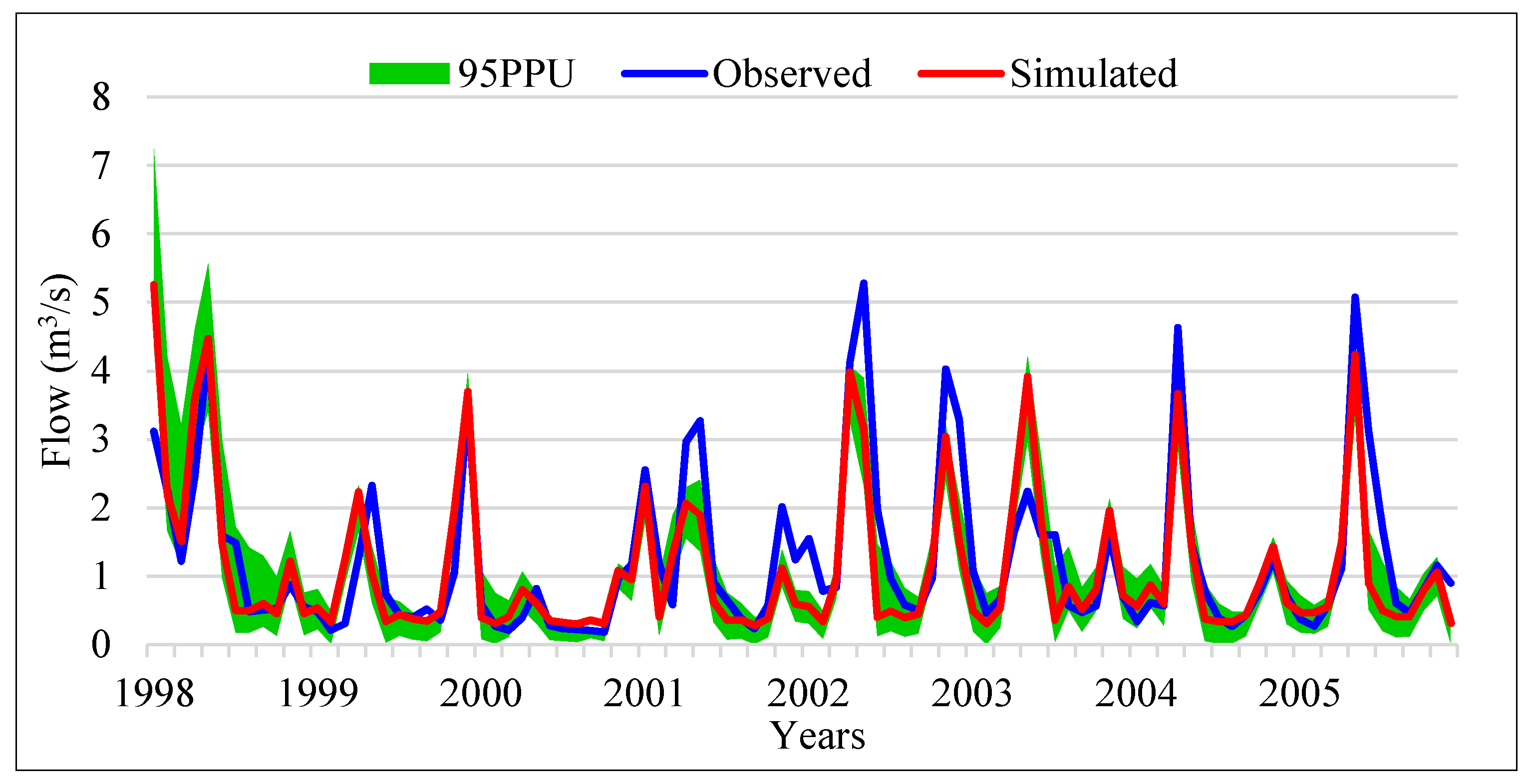
The objective function was achieved after five iterations of 500 simulations in each run. The observed data were incorporated within 70% of the 95% prediction uncertainty (95PPU)). Calibration results showed that p and r factors were about 0.7. According to [36], a p-factor greater than 0.70 and r-factor less than 1.5 show that the model is accurate in simulating streamflow. Thus, the results show that the model accurately simulated the biophysical processes influencing flow in the study area.
The statistical parameters, Nash Sutcliffe (NS), coefficient of determination (R2), and percent bias (PBIAS) were found to be 0.66, 0.69, and 10.3, respectively. Studies have shown that NS and R2 values close to 1 indicate a good fit between the observed and model results [37]. Other research indicated that the SWAT model can be judged as satisfactory if the NS value is greater than 0.5 and PBIAS is within ±25% during calibration for stream flow [37]. Therefore, in the present study, the model was considered to accurately predict stream flow in the catchment area.
Figure 4 illustrates the monthly observed and simulated streamflow between 1998 and 2005. The model closely matched the low flows well but, at some points, underestimated the high flows. Similar observations were reported in other studies using the SWAT-CUP model [38,39]. Other research indicated that the model does not accurately predict high flows and hence the simulated high flow events are underestimated [40].
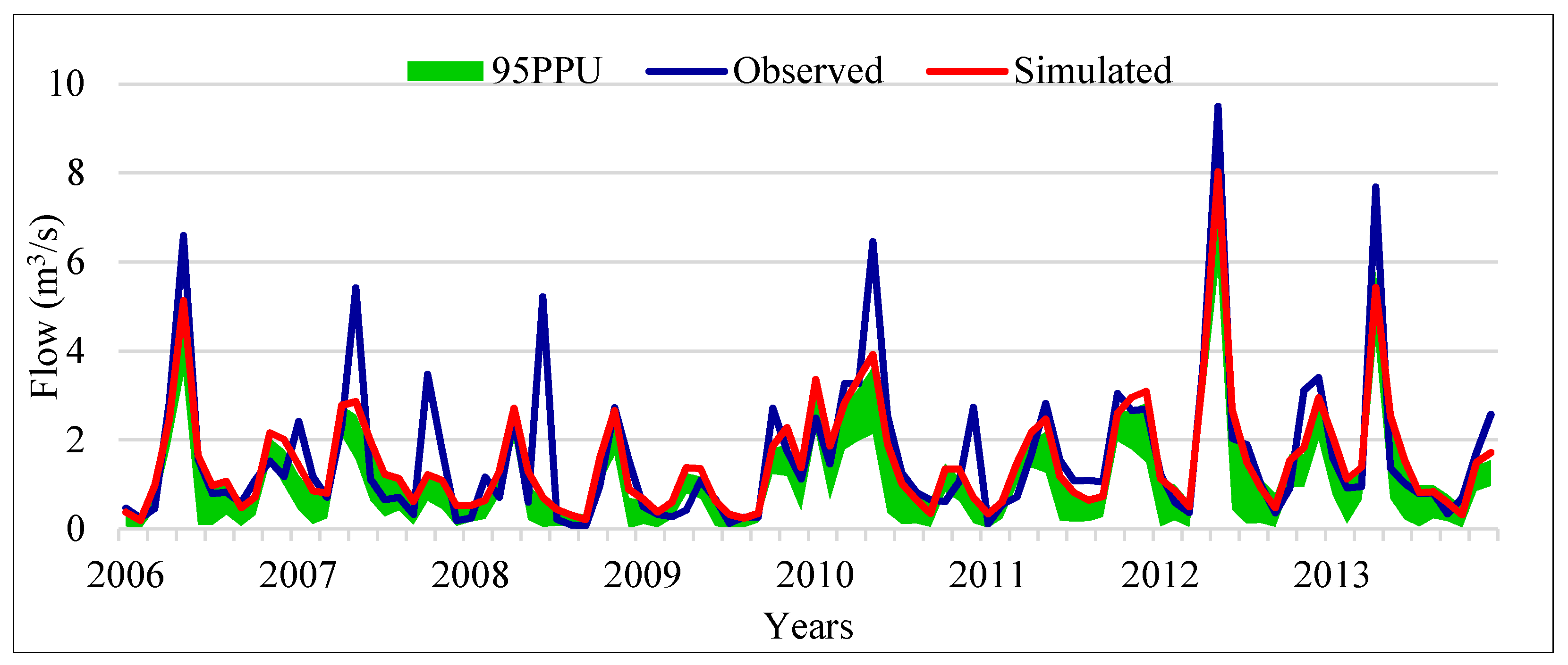
The calibrated parameters and their uncertainty range were used for the validation of streamflow between 2006 and 2013, as shown in Figure 5. The validation was considered satisfactory after one iteration of 500 simulations. The NS, R2, and PBIAS were found to be 0.7, 0.8, and 7, respectively. The p-factor and r-factor for the validation period were 0.6 and 0.5, respectively. The NS, R2, and PBIAS improved after the validation, but the p-factor was reduced by 9%. However, the p-value was greater than 0.5, which implies that 61% have been incorporated by the 95PPU. The calibration results also show that the low flows have higher calibration uncertainty than the high flows, as shown by the 95PPU.
A scatter plot of the observed and predicted streamflow using the calibrated parameters was plotted and an R2 of 0.6 was obtained, which was not very high but implied that the model was able to simulate streamflow correctly, both spatially and temporally (Figure 6). Similar studies have also recommended the use of observed data not considered in calibration processes in order to make simulations more representative and realistic and also ensure reliable performance of the hydrological process within the catchment.
Sedimentation data from a reservoir bathymetric survey conducted in 2011 were used to calibrate the model for sediments [28]. The study indicated that the average sediment inflow into the downstream Masinga reservoir is 5 Mt/year. Thika-Chania catchment contributes 1.8 Mt/year. (21 t/ha/year), which represents 36% of sediment inflow into Masinga reservoir [22]. Calibration of sediments involved adjusting the parameters that were found to be sensitive to sediment variation.
The mean annual sediment outflow from the catchment was compared with the simulated sediment yield. The model simulated annual sediment yield from the entire catchment of 22 t/ha. These results closely matched the observed sediment yield (21 t/ha/year) at the outlet of the catchment. Validation of the model was conducted at the upstream reservoirs (Thika and Sasumua dam). It was found that the average annual sediment yield in Sasumua and Ndakaini dam was 0.6 and 0.7 t/ha, respectively. According to the bathymetric survey, the two reservoirs were found to have an approximate annual sedimentation rate of 0 Mt/ha [29]. The model was further compared with the results obtained from a sediment yield study in Sasumua catchment [41]. The latter found that the average annual sediment yield from Sasumua (sub-basin 1, 2, 3, 4, 5, 6, 10, 11) is 10 t/ha.
The model simulated an annual sediment yield of 11 t/ha, which closely matched that observed at Sasumua sub-basin. Therefore, the model was considered satisfactory in terms of simulating sediment across the catchment. This methodology had been applied elsewhere in data-scarce regions to calibrate the SWAT model for sediment [16,41].
The base scenario showed that the average sediment yield from the catchment was 22 t/ha/year. Agricultural and bare areas were observed to have the highest sediment yield and were classified between high and very severe [42]. Tea-growing zones had relatively smaller sediment yield. This could be attributed to the extensive ground cover in tea zones. Those areas with the largest percentage of forest had slight sediment yield. It was observed that the high sediment yield from different sub-basins could be attributed to the type of land use, soil type, and high slopes. Other research conducted in a similar region has shown that coffee- and corn-growing zones have the highest sediment yield [32].
The model results showed that the base annual total water yield was 922 mm, where surface and baseflow were 202 mm and 638 mm, respectively. These results formed the base scenario for evaluating the impacts of soil conservation methods on water and sediment yield.
3.2. Contour Farming Impact on Sediment and Water Yield
Contour farming reduced sediments by 35.8% from the base scenario value of 22 t/ha/year. Figure 7 shows a map of the percent sediment reduction after contour farming simulation. It shows that sub-catchments 1, 6, 8, and 7 indicated sediment yield reduction between 50% and 60%. According to [41], the sub-catchments are characterized by intensive farming of horticultural crops at a small scale, thus practicing contour farming would be effective in improving regulatory and provisioning ecosystem services. Similarly, sub-catchments 35, 36, and 37 that grow coffee, showed a high percent of reduction in sediment yield from the baseline simulation values.
The surface runoff generated from the catchment reduced by 16% from 202 mm, while the baseflow increased by 3%. The shallow groundwater aquifers increased by 8% from a mean of 77 mm. While surface runoff was decreased, the total water yield decreased by only 0.6%. This shows that contour farming is able to reduce the runoff generated from the fields by increasing the amount of water infiltrating into the soil layers.
Increased baseflow implies an increment of water in the shallow aquifer that would gradually be released to the streams during the dry season. Increased water infiltration would prevent fertilizers and pesticides from being washed into the water bodies, thus increasing water quality and crop production since fertilizers are retained in the agricultural land. Contour farming is not labor-intensive, and the cost of implementation is also low compared to structural practices [43]. Evaluation of contour farming by [15] showed a reduction of sediment yield from Bosque River catchment by 28% to 67%. Contour farming would reduce sediment yield at the outlet of Sasumua sub-basin by 49% [41]. Studies done in Northeast Iowa indicated that contour farming reduced flow by 4% and sediment yield by 34% [44]. These studies agree with the finding of this research that contour farming is effective at reducing surface runoff and sediments yielded from the uplands area.
3.3. Filter Strips’ Impacts on Sediment and Water Yield
Results showed that filter strips of 5 m width would reduce the average annual sediment yield from the catchment by 54% (Figure 8). However, total water yield did not change from the base simulation. Unlike contour farming, filter strips allow surface runoff to pass with a reduced amount of sediment. The filter width of a vegetative strip determines the trapping efficiency for sediment removal from surface runoff. Implementing a 3-m filter strip would reduce sediment yield by 46%. A 10-m strip, on the other hand, reduced sediment yield by 66%, while a 30-m strip reduced it by 88%. Similar trends in sediment removal efficiency have been observed in other studies [45]. Moriasi et al. observed that the rate of removal of sediment from a 3-m filter strip removed more than 70% of sediment [37], while a 10-m strip trapped more than 85% from the surface runoff in northeast Iowa. Similar to the findings of [46], this study found that, when increasing the width of buffer strips beyond 30 m, the annual average sediment reduction would be insignificant compared to the narrower strips.
Results showed that the effectiveness of reducing sediment yield from the catchment increases with the increase in width of the filter strip. However, the amount of sediment trapped does not increase by bigger percentages beyond the 10-m filter strip. Similar trends in sediment removal efficiency were observed in other studies [45]. Another study [47] reported that most of the soil particles greater than 40 micrometers in diameter are removed within the first 5 m of the filter strips. This can be attributed to the high sediment reduction within the first 3 m of filter strip width in the current study. According to [34], the filter width of a vegetative strip determines the trapping efficiency for sediment removal from surface runoff. Sediment characteristics, slope of the filter, and the underlying soil characteristics also influence the trapping efficiency.
According to the national land use guidelines of Kenya, a minimum of 2 m should be left on both sides of the river as riparian area and a minimum of 30 m should be left uncultivated from the highest water mark during peak flows [48]. If these guidelines are followed, the amount of sediment reaching waterbodies would be significantly reduced. Performance testing of vegetative filter strips was conducted in Canada and revealed that the efficiency of sediment removal from overland flow varies by 50–98% with an increase in filter strip width [47,49]. Other research conducted in Ethiopia found that filter strips reduced sediment from the base simulation value by 55–84% [19].
3.4. Combination of Contour Farming and Filter Strips
Based on the average land sizes in the catchment and the integrated land use guidelines [49], it was assumed that a 3-m filter strip would be implemented on a wide range in the catchment.
The implementation of contour farming together with a 3-m filter strip would reduce sediment yield at the outlet of the catchment by 63%. This is an increment of 27% compared to implementing contour farming individually. A 3-m filter strip would reduce 46% of sediments produced in the catchment but, when combined with contour farming, a further 17% reduction in sediment yield was achieved. This shows that the combination of two conservation practices can significantly increase sediment yield reduction. However, after integrating the conservation method, the total water yield for either practice remains unchanged.
The land use guidelines in the study area further stipulate that a minimum of 10 m filter strip should be left between quarries and rivers. As such, 5-m and 10-m combinations of contour farming and grass strips were evaluated. Results indicated that a 5-m grass strip‒contour farming combination reduced sediment yield at the catchment outlet by 67%, while a 10-m grass strip combination reduced sediment by 74%. This shows that increasing the filter width beyond 10 m and integrating it with contour farming, can reduce sediment yield by more than 70%. Similar results have been observed in other studies where contour farming was implemented together with 5-m filter strips and reduced sediment loading by 73% from the baseline value [27]. Mwangi et al. [33] evaluated the impact of a 10-m filter strip combined with contour farming and reported sediment reduction of 41% on a catchment of 110 km2. Therefore, from this analysis, contour farming and filter strips can effectively be used to restore and improve ecosystem services.
4. Conclusions
Intensive land cultivation and increased surface runoff from degraded areas have increased soil erosion and subsequent sedimentation in reservoirs in Kenya. Therefore, specific conservation measures are needed to tackle these problems. This paper aimed at evaluating the impacts of contour farming, grass strips, and filter strips on sediment and water yield at Thika-Chania catchment using a SWAT model. Calibration and validation of the model were conducted using SWAT-CUP model and obtained good results. However, there were limited observed data to calibrate the model for sediment. Contour farming and grass strip implementation in 50% of the catchment resulted in a significant reduction of sediment yield in the catchment. Filter strips with a width of 3 m were assumed to be implemented in the catchment. Results showed that 46% of sediments would be reduced from the base annual average simulation value of 22 t/ha. More sediment reduction was observed to increase with an increase in filter widths. However, reduction beyond 10 m width was small compared to the first 5 m. Implementation of contour farming resulted in a decline of sediment yield by 36%. Contour farming resulted in a decline of stream flow by 16.4%, while the baseflow increased by 3%. The total water yield decreased by 0.6% for contour farming. Moreover, contour farming together with 3-m filter strips reduced sediment yield by 63%. Integration of the two conservation methods resulted in more sediment reduction than when individual practices were implemented. It was also noted that filter strips had no significant impact on water yield, whether implemented individually or integrated with contour farming. The paper concluded that good management practices are necessary for the sustainability of the ecosystem services and to enhance agricultural production levels in the catchment; however, the effectiveness of a given soil and water management method differs from one area to the other due to variability in different parameters like weather, soil, extent of the implementation, and topography.
Author Contributions
Methodology, J.N.G., J.S.; Analysis, J.N.G., J.S.; Model Preparation & Calibration, J.N.G.; Resources, J.N.G., K.A.M., J.S.; Data, J.N.G., J.S.; Writing-Original Draft Preparation J.N.G., Writing-Review, Editing and Submission, K.A.M; Supervision, K.A.M.; Open Access Publication, K.A.M.
Funding
This research received no external funding.
Acknowledgments
The authors thank the Center for Middle Eastern Studies at Lund University for funding the publication of this paper through the MECW program.
Conflicts of Interest
The authors declare no conflict of interest.
References
- Cohen, M.J.; Brown, M.T.; Shepherd, K.D. Estimating the environmental costs of soil erosion at multiple scales in Kenya using emergy synthesis. Agric. Ecosyst. Environ. 2006, 114, 249–269. [Google Scholar] [CrossRef]
- Angima, S.D.; Stott, D.E.; Neill, M.K.O.; Ong, C.K.; Weesies, G.A. Soil erosion prediction using RUSLE for central Kenyan highland conditions. Agric. Ecosyst. Environ. 2003, 97, 295–308. [Google Scholar] [CrossRef]
- Mourad, K.A.; Alshihabi, O. Assessment of future Syrian water resources supply and demand by the WEAP model. Hydrol. Sci. J. 2015, 61, 393–401. [Google Scholar] [CrossRef]
- Metobwa, O.G.M.; Mourad, K.A.; Ribbe, L. Water demand simulation using WEAP 21: A Case Study Mara River Basin, Kenya. Int. J. Nat. Resour. Ecol. Manag. 2018, 3, 9–18. [Google Scholar] [CrossRef]
- Mourad, K.; Berndtsson, R.; Abu-El-Sha’r, W.; Qudah, M.A. Modeling tool for air stripping and carbon adsorbers to remove trace organic contaminants. Int. J. Therm. Environ. Eng. 2012, 4, 99–106. [Google Scholar] [CrossRef]
- Khorchani, N.; Mourad, K.A.; Ribbe, L. Assessing the impact of land-use change to the hydrological response in Mellegue river, Tunisia. Curr. Environ. Eng. 2018, 5, 125–135. [Google Scholar] [CrossRef]
- Mourad, K.A.; Berndtsson, R. Syrian water resources between the present and the future. Air Soil Water Res. 2011, 4, 93–100. [Google Scholar] [CrossRef]
- Mourad, K.A.; Berndtsson, R. Water status in the Syrian water basins. Open J. Mod. Hydrol. 2012, 2, 15–20. [Google Scholar] [CrossRef]
- Arnold, J.G.; Moriasi, D.N.; Gassman, P.W.; Abbaspour, K.C.; White, M.J.; Srinivasan, R.; Jha, M.K. SWAT: Model use, calibration and validation. Am. Soc. Agric. Boil. Eng. 2012, 55, 1491–1508. [Google Scholar]
- Ajwang’, O.R.; Kitaka, N.; Oduor, O.S. Assessment of provisioning and cultural ecosystem services in natural wetlands and rice fields in Kano floodplain, Kenya. Ecosyst. Serv. 2016, 21, 166–173. [Google Scholar] [CrossRef]
- Morgan, R.P.C. Soil Erosion & Conservation, 3rd; Wiley-Blackwell: Malden, MA, USA, 2005. [Google Scholar]
- Quinton, J.N.; Catt, J.A. The effects of minimal tillage and contour cultivation on surface runoff, soil loss and crop yield in the long-term Woburn Erosion Reference Experiment on sandy soil at Woburn, England. Soil Use Manag. 2004, 20, 343–349. [Google Scholar] [CrossRef]
- Tadesse, L.D.; Morgan, R.P.C. Contour grass strips: A laboratory simulation of their role in erosion control using live grasses. Soil Technol. 1996, 9, 83–89. [Google Scholar] [CrossRef]
- Yuan, Y.; Mbonimpa, E.G.; Nash, M.S.; Mehaffey, M.H. Sediment and total phosphorous contributors in Rock River watershed. J. Environ. Manag. 2014, 133, 214–221. [Google Scholar] [CrossRef]
- Tuppad, P.; Kannan, N.; Srinivasan, R.; Rossi, C.G.; Arnold, J.G. Simulation of agricultural management alternatives for watershed protection. Water Resour. Manag. 2010, 24, 3115–3144. [Google Scholar] [CrossRef]
- Vogl, A.L.; Bryant, B.P.; Hunink, J.E.; Wolny, S.; Apse, C.; Droogers, P. Valuing investments in sustainable land management in the Upper Tana River basin, Kenya. J. Environ. Manag. 2016, 195, 78–91. [Google Scholar] [CrossRef] [PubMed]
- Cho, J.; Lowrance, R.R.; Bosch, D.D.; Strickland, T.C.; Her, Y.; Vellidis, G. Effect of watershed subdivision and filter width on swat simulation of a coastal plain watershed. J. Am. Water Resour. Assoc. 2010, 46, 586–602. [Google Scholar] [CrossRef]
- Droogers, P.; Hunink, J.E.; Kauffman, J.H.; Van Lynden, G.W.J. Costs and Benefits of Land Management Options in the Upper Tana, Kenya Using the Water Evaluation and Planning System—WEAP; ISRIC—World Soil Information: Wageningen, The Netherlands, 2011. [Google Scholar]
- Herweg, K.; Ludi, E. The performance of selected soil and water conservation measures—Case studies from Ethiopia and Eritrea. Catena 1999, 36, 99–114. [Google Scholar] [CrossRef]
- Parajuli, P.B.; Mankin, K.R.; Barnes, P.L. Applicability of targeting vegetative filter strips to abate fecal bacteria and sediment yield using SWAT. Agric. Water Manag. 2008, 95, 1189–1200. [Google Scholar] [CrossRef]
- Archer, D. Suspended sediment yields in the Nairobi area of Kenya and environmental controls. In Proceedings Exeter Symposium; IAHS Publishers: Wallingford, UK, 1996; pp. 37–48. [Google Scholar]
- Hunink, J.E.; Droogers, P. Impact Assessment of Investment Portfolios for Business Case Development of the Nairobi Water Fund in the Upper Tana River, Kenya; FutureWater: Wageningen, The Netherlands, 2015; Volume 31. [Google Scholar]
- Leisher, C.; Makau, J.; Kihara, F.; Kariuki, A.; Sowles, J.; Courtemanch, D.; Njugi, G.; Apse, C. Upper Tana-Nairobi Water Fund Monitoring and Evaluation Plan. 2013. Available online: https://s3.amazonaws.com/tnc-craft/library/Upper-Tana-ME-Plan-v7.pdf?mtime=20180218223009 (accessed on 20 August 2018).
- Hunink, J.E.; Immerzeel, W.W.; Droogers, P.; Kauffman, J.H. Impacts Land Manag. Options Up. Tana, Kenya Using Soil Water Assess: Tool—SWAT. 2011. Available online: https://www.researchgate.net/publication/254906365 (accessed on 21 September 2018).
- Gathagu, J.N.; Mutua, B.M.; Mourad, K.A.; Oduor, B.O. Uncertainty analysis and calibration of SWAT model for estimating impacts of conservation methods on streamflow and sediment yield in Thika River catchment, Kenya. Int. J. Hydrol. Res. 2018, 3, 1–11. [Google Scholar] [CrossRef]
- Hunink, J.E.; Droogers, P. Physiographical Baseline Survey for the Upper Tana Catchment: Erosion and Sediment Yield Assessment; FutureWater: Wageningen, The Netherlands, 2011; Volume 31. [Google Scholar]
- Mwangi, H.M. Evaluation of the Impacts of Soil and Water Conservation Practices on Ecosystem Services in Sasumua Watershed, Kenya, Using SWAT Model; Jomo Kenyatta University of Agriculture and Technology: Juja, Kenya, 2011. [Google Scholar]
- Humberto, B.; Rattan, L. Principles of Soil Conservation and Management; Springer: Dordrecht, The Netherlands, 2008. [Google Scholar] [CrossRef]
- Jha, M.; Gassman, P.W.; Secchi, S.; Gu, R.; Arnold, J. Effect of watershed subdivision on SWAT Flow, sediment, and nutrient predictions. J. Am. Water Resour. Assoc. 2004, 40, 811–825. [Google Scholar] [CrossRef]
- Jabro, J.D. Estimation of saturated hydraulic conductivity of soils from particle size distribution and bulk density data. Am. Soc. Agric. Eng. 1992, 35, 557–560. [Google Scholar] [CrossRef]
- Neitsch, S.L.; Arnold, J.G.; Kiniry, J.R.; Williams, J.R. Soil and Water Assessment Tool Theoretical Documentation. 2011. Available online: https://swat.tamu.edu/media/99192/swat2009-theory.pdf (accessed on 21 September 2018).
- Hunink, J.E.; Niadas, I.A.; Antonaropoulos, P.; Droogers, P.; de Vente, J. Targeting of intervention areas to reduce reservoir sedimentation in the Tana catchment (Kenya) using SWAT. Hydrol. Sci. J. 2013, 58, 600–614. [Google Scholar] [CrossRef] [Green Version]
- Mwangi, J.K.; Shisanya, C.A.; Gathenya, J.M.; Namirembe, S.; Moriasi, D.N. A modeling approach to evaluate the impact of conservation practices on water and sediment yield in Sasumua Watershed, Kenya. Soil Water Conserv. 2015, 70, 75–90. [Google Scholar] [CrossRef]
- Arabi, M.; Frankenberger, J.R.; Engel, B.A.; Arnold, J.G. Representation of agricultural conservation practices with SWAT. Hydrol. Process. 2008, 22, 3042–3055. [Google Scholar] [CrossRef]
- Wischmeir, W.H.; Smith, D.D. Predicting Rainfall Erosion Losses—A Guide to Conservation Planning; U.S. Department of Agriculture: Washington, DC, USA, 1978.
- Abbaspour, K.C. SWAT-CUP: SWAT Calibration and Uncertainty Programs. 2015. Available online: https://swat.tamu.edu/media/114860/usermanual_swatcup.pdf (accessed on 21 September 2018).
- Moriasi, D.N.; Arnold, J.G.; Liew, M.W.; Van Bingner, R.L.; Harmel, R.D.; Veith, T.L. Model evaluation guidelines for systematic quantification of accuracy in watershed simulations. Am. Soc. Agric. Boil. Eng. 2007, 50, 885–900. [Google Scholar]
- Meaurio, M.; Zabaleta, A.; Angel, J.; Srinivasan, R.; Antigüedad, I. Evaluation of SWAT models performance to simulate streamflow spatial origin. The case of a small forested watershed. J. Hydrol. 2015, 525, 326–334. [Google Scholar] [CrossRef]
- Rostamian, R.; Aazam, J.; Afyuni, M.; Farhad, S.; Heidarpour, M.; Jalalian, A.; Abbaspour, K. Application of a SWAT model for estimating runoff and sediment in two mountainous basins in central Iran. Hydrol. Sci. J. 2010, 53, 977–988. [Google Scholar] [CrossRef]
- Tolson, B.A.; Shoemaker, C.A. Watershed Modeling of the Cannonsville Basin Using SWAT2000: Model Development, Calibration and Validation for the Prediction of Flow, Sediment and Phosphorus Transport to the Cannonsville Reservoir; Cornell University Library: Ithaca, NY, USA, 2004. [Google Scholar]
- Mwangi, H.M.; Gathenya, J.M.; Mati, B.M.; Mwangi, J.K. Evaluation of Agricultural Conservation Practices on Ecosystem Services in Sasumua Watershed, Kenya Using SWAT Model. 2013, pp. 659–673. Available online: http://ir.jkuat.ac.ke/handle/123456789/994 (accessed on 21 September 2018).
- Singh, G.; Babu, R.; Narain, P.; Bhushan, L.S.; Abrol, I.I. Soil erosion rates in India. J. Soil Water Conserv. 1992, 1, 97–99. [Google Scholar]
- Phomcha, P.; Wirojanagud, P.; Vangpaisal, T.; Thaveevouthti, T. Modeling the impacts of alternative soil conservation practices for an agricultural watershed with the SWAT model. Procedia Eng. 2012, 32, 1205–1213. [Google Scholar] [CrossRef]
- Gassman, P.W.; Osei, E.; Saleh, A.; Rodecap, J.; Norvell, S.; Williams, J. Alternative practices for sediment and nutrient loss control on livestock farms in northeast Iowa. Agric. Ecosyst. Environ. 2006, 117, 135–144. [Google Scholar] [CrossRef]
- Yuan, Y.; Bingner, R.A.; Locke, M.A. Review of effectiveness of vegetative buffers on sediment trapping in agricultural areas. Ecohydrology 2009, 2, 321–336. [Google Scholar] [CrossRef]
- Vaché, K.B.; Eilers, J.M.; Santelmann, M.V. Water quality modeling of alternative agricultural scenarios in the U.S. Corn Belt. J. Am. Water Resour. Assoc. 2003, 38, 773–787. [Google Scholar] [CrossRef]
- Gharabaghi, B.; Rudra, R.P.; Whiteley, H.R.; Dickinson, W.T. Performance testing of vegetative filter strips. Am. Soc. Civ. Eng. 2004, 1–9. [Google Scholar]
- National Environmental Management Authority (NEMA). Integrated National Landuse Guidelines; NEMA: Nairobi, Kenya, 2011.
- Helmmers, M.; Thomas, I.; Dosskey, M.G.; Dabney, S.M.; Strock, J. Buffers and vegetative filter strips. In Upper Mississippi River Sub-basin Hypoxia Nutrient Committee (UMRSHNC); National Forest Service: Washington, DC, USA, 2008; pp. 43–58. [Google Scholar]
Figure 1.
Thika-Chania catchment area.

Figure 2.
Land use at Thika-Chania catchment.

Figure 3.
Slope variation at Thika-Chania catchment.

Figure 4.
Monthly streamflow calibration results for gauging station 4CB05.

Figure 5.
Monthly streamflow validation results for gauging station 4CB05.

Figure 6.
A scatterplot of the observed and simulated streamflow at gauging station 4CB04.

Figure 7.
Simulation results of sediment reduction after contour farming.

Figure 8.
Simulation of annual sediment yield and sediment reduction at different filter widths.


Table 1.
Data used in the SWAT model setup.
| Datasets | Detail |
|---|---|
| Digital elevation model | 30 m resolution |
| SOTER-UT soils map | Scale 1:250,000 |
| Upper Tana Land use map (2009) | 30 m resolution |
| Meteorological data | Daily (1996–2013) |
| Streamflow data | Daily (1996–2013) |
| Sediments load/Turbidity data | Point data 2010 |
| Bathymetric survey data | Thika dam, Sasumua dam, Masinga dam |
© 2018 by the authors. Licensee MDPI, Basel, Switzerland. This article is an open access article distributed under the terms and conditions of the Creative Commons Attribution (CC BY) license (http://creativecommons.org/licenses/by/4.0/).
Share and Cite
MDPI and ACS Style
Gathagu, J.N.; Mourad, K.A.; Sang, J. Effectiveness of Contour Farming and Filter Strips on Ecosystem Services. Water 2018, 10, 1312. https://doi.org/10.3390/w10101312
AMA Style
Gathagu JN, Mourad KA, Sang J. Effectiveness of Contour Farming and Filter Strips on Ecosystem Services. Water. 2018; 10(10):1312. https://doi.org/10.3390/w10101312
Chicago/Turabian StyleGathagu, John Ng’ang’a, Khaldoon A. Mourad, and Joseph Sang. 2018. "Effectiveness of Contour Farming and Filter Strips on Ecosystem Services" Water 10, no. 10: 1312. https://doi.org/10.3390/w10101312
Note that from the first issue of 2016, this journal uses article numbers instead of page numbers. See further details here.