Article

Analysis of Milk Production and Failure Data: Using Unit Exponentiated Half Logistic Power Series Class of Distributions

by
Safar M. Alghamdi
1,
Mansour Shrahili
2,
Amal S. Hassan
3,*,
Rokaya Elmorsy Mohamed
4,
Ibrahim Elbatal
5 and
Mohammed Elgarhy
6
1
Department of Mathematics and Statistics, College of Science, Taif University, P.O. Box 11099, Taif 21944, Saudi Arabia
2
Department of Statistics and Operations Research, College of Science, King Saud University, P.O. Box 2455, Riyadh 11451, Saudi Arabia
3
Faculty of Graduate Studies for Statistical Research, Cairo University, 5 Dr. Ahmed Zewail Street, Giza 12613, Egypt
4
Department of Mathematics, Statistics and Insurance, Sadat Academy for Management Sciences, Cairo 11728, Egypt
5
Department of Mathematics and Statistics, Faculty of Science, Imam Mohammad Ibn Saud Islamic University (IMSIU), Riyadh 11432, Saudi Arabia
6
Mathematics and Computer Science Department, Faculty of Science, Beni-Suef University, Beni-Suef 62521, Egypt
*
Author to whom correspondence should be addressed.
Symmetry 2023, 15(3), 714; https://doi.org/10.3390/sym15030714
Submission received: 16 February 2023 / Revised: 5 March 2023 / Accepted: 10 March 2023 / Published: 13 March 2023

Abstract

:
The unit exponentiated half logistic power series (UEHLPS), a family of compound distributions with bounded support, is introduced in this study. This family is produced by compounding the unit exponentiated half logistic and power series distributions. In the UEHLPS class, some interesting compound distributions can be found. We find formulas for the moments, density and distribution functions, limiting behavior, and other UEHLPS properties. Five well-known estimating approaches are used to estimate the parameters of one sub-model, and a simulation study is created. The simulated results show that the maximum product of spacing estimates had lower accuracy measure values than the other estimates. Ultimately, three real data sets from various scientific areas are used to analyze the performance of the new class.

1. Introduction

Recently, academics have become more interested in the creation of new univariate distributions, which are frequently used in statistics and related fields due to theoretical considerations, practical applications, or both. By combining a specific useful lifetime with truncated discrete distributions, compounding is a practical method for producing new distributions. The fundamental principle underlying the construction of these compounding distributions is that the lifetime of a system with V components and a positive continuous random variable Z i which represents the lifetime of the ith component, can be represented by a non-negative random variable Z = min( Z 1 , , Z V ) if the components are in a series, or Z = max( Z 1 , , Z V ) if the components are in parallel. In both situations, it is believed that the continuous random variables Z i are independent of V.
In recent decades, several studies have examined the creation of new probabilistic families by combining various distributions and the power series (PS) model. Most of the works have been motivated by systems consisting of series or parallel components. Most of the generalization is motivated by a system consisting of a series of components. For instance, Morais and Barreto-Souza [1] presented the Weibull–PS class, discussed some statistical properties, thought about estimation using the maximum likelihood (ML) approach, and provided data analysis. Similar work was presented by Mahmoudi and Jafari [2] and Silva et al. [3] for the generalized exponential-PS and extended Weibull–PS classes, respectively, using generalized exponential and extended Weibull. Jafari and Tahmasebi [4] discussed the class of the Gompertz PS, presented some properties, discussed the ML estimation procedure, and presented a simulation study for complete and censored data. Elbatal et al. [5] introduced the class of exponential Pareto-PS. The Burr XII-PS class, as well as the Burr–Weibull–PS class, were introduced by Silva and Corderio [6] and Oluyede et al. [7]. Alizadeh et al. [8] investigated exponentiated power Lindley-PS class, discussed ML estimation, provided formulas for the elements of the Fisher information matrix, and examined real data sets. Alkarni [9] introduced the generalized inverse Lindley PS class in his paper. The new Lindley–Burr XII PS class was recommended by Makubate et al. [10], along with discussions of the properties class, estimation of the parameters, and real-world applications. The inverse gamma PS class was created by Rivera et al. [11]; estimation and data analysis are also provided. The inverted exponentiated Lomax PS class was proposed by Hassan et al. [12], who also explained the properties class, estimated the parameter, and gave real data applications.
On the other hand, lifetime models and the PS distribution have been compounded to present numerous compound distributions by complementary risk motivation. These models were motivated by a parallel system with an unknown number of components. For instance, Flores et al. [13] introduced the complementary exponential PS class, explained the class properties, discussed parameter estimators, and offered real data applications. Hassan et al. [14] suggested the complementary Poisson Lindley-PS class and provided estimation and application to real data. Bagheri et al. [15] developed the generalized modified Weibull–PS class, which evaluated the estimation process, offered a formula for the components of the Fisher information matrix, and provided real data analysis. The complementary exponentiated inverted Weibull–PS class was investigated by Hassan et al. [16], which also examined the parameter estimators and supplied real data analysis. Oluyede et al. [17] provided the generalized exponentiated PS class. The power function–PS class was introduced by Hassan and Assar [18], who also covered the class’s characteristics, parameter estimators, and real-world applications.
The growth of unit distributions has accelerated recently. These distributions focus on modeling a wide variety of events using information having values between zero and one, such as proportions, probabilities, and percentages. According to Papke and Wooldridge [19], many economic settings naturally produce variables with a range of zero to one, such as the percentage of total weekly hours worked, the percentage of income spent on non-durable consumption, the participation rates in pension plans, industry market shares, television viewership, the percentage of the land area allocated to agriculture, etc. To represent lifetime data in reliability analysis, many authors use continuous models with finite support. Physical considerations, such as a component’s finite lifetime or the bounded signals present in industrial systems, are frequently the driving forces behind this (see, for instance, Jiang [20] and Dedecius and Ettler [21]). For models established on the unit interval, reliability should be expressed as a percentage or ratio [22], in order to get results that are believable Today’s unit distributions are largely produced by correctly adjusting traditional distributions. The unit Weibull and the new unit Lindley are developed by [23,24]. The unit exponentiated half logistic (UEHL) developed by Hassan et al. [25] has lately been published, and it has caught our interest. The following formulas define the cumulative distribution function (CDF) and probability density function (PDF) of the UEHL distribution:
G ( z ; a , b ) = 1 1 z a 1 + z a b , 0 < z < 1 ,
and
g ( z ; a , b ) = 2 a b ( 1 + z a ) ( b + 1 ) z a 1 ( 1 z a ) b 1 , 0 < z < 1 ,
where a , b R + , are the scale and shape parameters, respectively. They investigated some of the UEHL distribution’s characteristics and discussed the parameter estimators using different estimation methods.
In the fields of biology and engineering, the compounding technique makes it possible to create flexible distributions with substantial physical significance. On the other hand, the bounded distributions concentrate on modeling a large range of events using data with values between zero and one. To our knowledge up to now, no compound family has been created based on unit distributions. So, our objective here is to introduce the unit exponentiated half logistic power series (UEHLPS) by taking into account a system with parallel components and combining UEHL and PS distributions. We provide a versatile class that includes a number of UEHL types of distributions combined with discrete distributions (truncated at zero). Various distributional properties including, quantile function, moments, entropy measure, Lorenz, and Bonferroni curves are presented. The parameters of one UEHL Poisson (UEHLP) model are estimated using some classical estimation techniques, including Cramer von Mises (CM), least squares (LS), weighed LS (WLS), ML, and the maximum product of spacings (MPS). The accuracy of the estimated estimators is investigated by a numerical simulation experiment. The potentiality of the UEHLP model is investigated by utilizing three real data sets from distinct scientific disciplines. In addition, Figure 1 depicts a detailed explanation of the work.
The creation of the UEHLPS class of distribution, which can be applied in a number of remarkable situations, is motivated by the fact that:
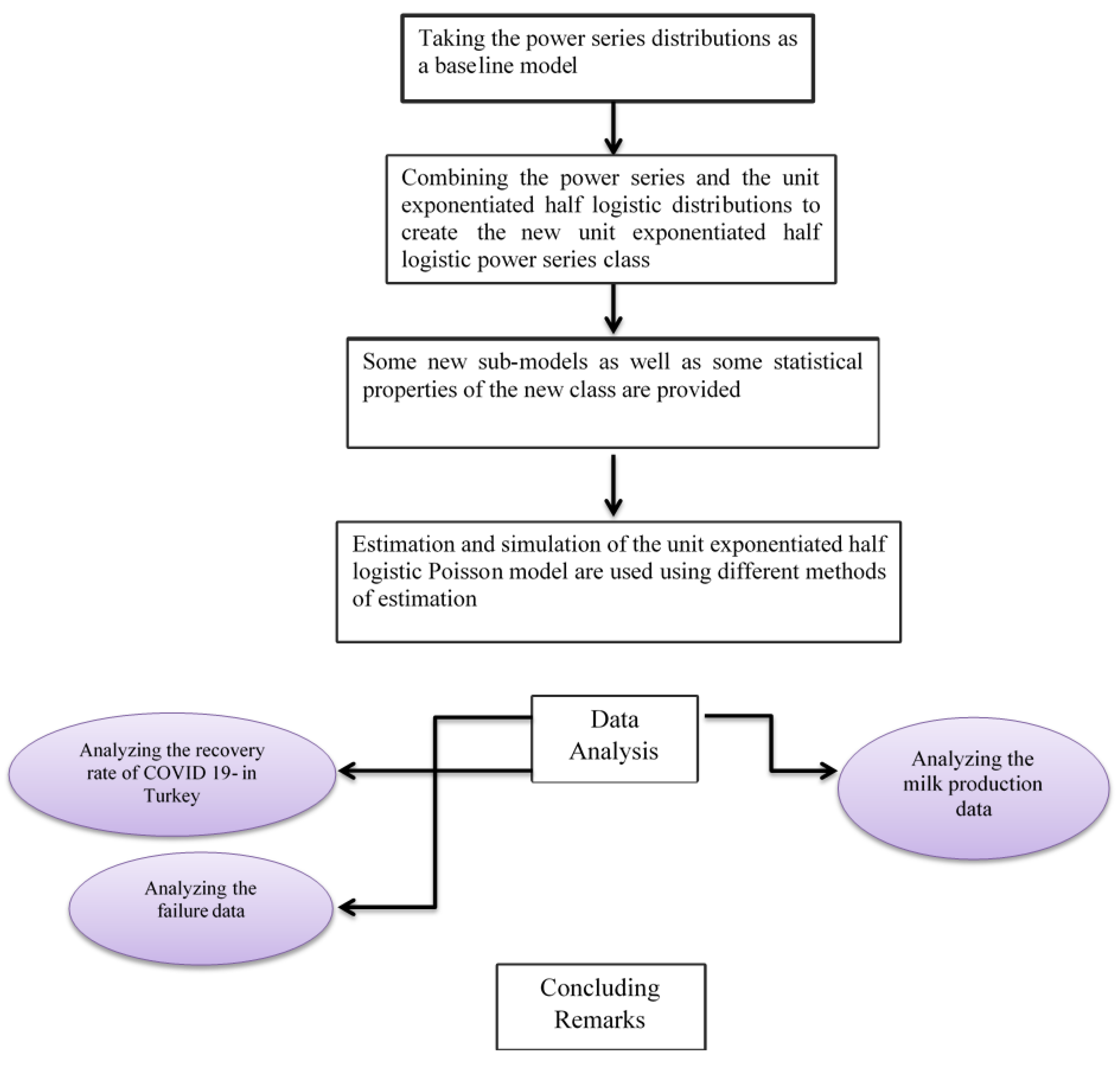
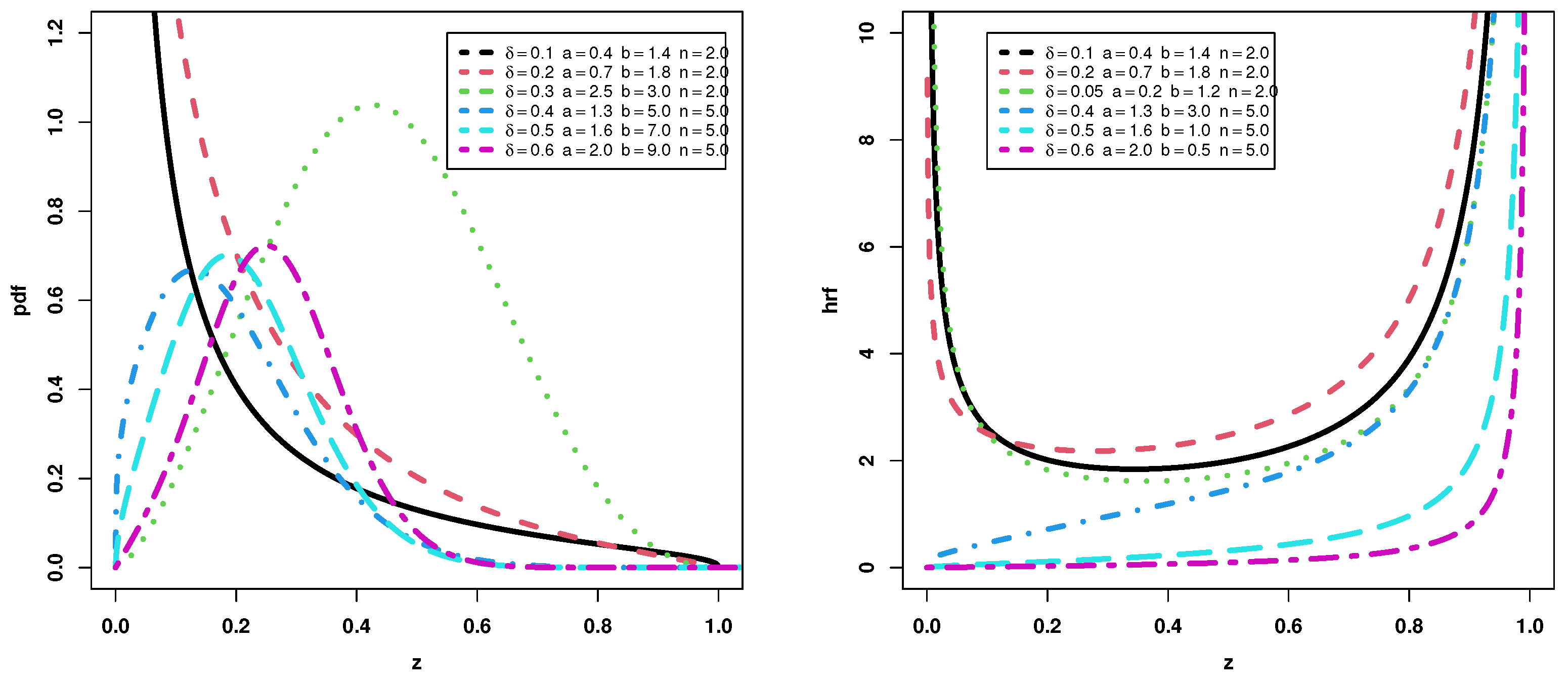
  • The UEHLPS class of distributions can appear in various industrial applications as a result of the stochastic reorientation Z = max( Z 1 , , Z V ).
  • The UEHLPS family of distributions can be used to roughly simulate the time until the last failure of a system composed of similar components that are operating in parallel.
  • The UEHLPS class of distributions exhibits a number of interesting non-monotonic failure rate phenomena, such as bathtub, increasing, decreasing, and J-shaped, which are more likely to be observed in real contexts.
The structure of this article is described as follows: The PDF, CDF, and hazard rate function (HF) of the UEHLPS class are provided in Section 2. Section 3 introduces the specific sub-models of the class. We give a few structural characteristics of the UEHLPS class in Section 4 and Section 5. Descriptions of different classical estimators of the UEHLP distribution parameters are given in Section 6. Section 7 and Section 8 describe numerical examination and real data analysis, respectively. The article is concluded in Section 9.

2. Formation of the New Class

In this section, we construct the class of the UEHLPS distributions by combining the UEHL distribution with the PS distribution. Let V be a zero-truncated discrete random variable having a PS with the following probability mass function (PMF)
P ( V = v ) = ς v δ v D ( δ ) , v = 1 , 2 , 3 ,
where ς v depends only on v , δ > 0 , is the scale parameter, D ( δ ) = v = 1 ς v δ v , D ( . ) and D ( . ) denote the first and second derivatives of D ( δ ) , respectively. We draw attention to the fact that the PMF in Equation (3) also matches the generalized PS distribution covered in Patil [26]. Several structural characteristics and statistical issues related to generalized PS were discovered by Patil [27,28].
Let Z = max Z i i = 1 V , the joint CDF is given by:
P ( Z z ; V = v ) = ς v δ v D ( δ ) 1 1 z a 1 + z a b v , 0 < z < 1 , v 1 .
The conditional CDF of Z V is given by:
H Z V = v ( z ) = G ( z ; a , b ) v = 1 1 z a 1 + z a b v .
So, the marginal CDF of (4) is given by
H ( z ; ϖ ) = v = 1 ς v δ v D ( δ ) 1 1 z a 1 + z a b v = 1 D ( δ ) v = 1 ς v δ 1 1 z a 1 + z a b v .
Hence the CDF of the UEHLPS class is as follows:
H ( z ; ϖ ) = 1 D ( δ ) D δ 1 Λ z , a , b , 0 < z < 1 ,
where Λ z , a , b = 1 z a 1 + z a b . A random variable with CDF(5) has UEHLPS class with parameters ϖ ( a , b , δ ) shall be denoted by Z UEHLPS ( ϖ ) .
The family of models in (5) can be physically interpreted as follows: Consider the case where a system, equipment, product, or component occurs due to the presence of an unknown number, say V, of protected components or a disease manifestation, which can be identified only after an unknown number of factors have been active. Suppose that Z i is the time to the failure of the device owing to the ith flaw, for i 1 , such that each Z i follows the UEHL distribution (1) and V is discrete PS distribution (3), then the distribution of the random variable Z i , which represents the time of last failure, is the distribution in (4).
The PDF of the UEHLPS class, for 0 < z < 1 , corresponding to (5) is:
h ( z ; ϖ ) = 2 a b δ ( 1 + z a ) ( b + 1 ) z a 1 ( 1 z a ) b 1 D δ 1 Λ z , a , b D ( δ ) .
The survival function (SF) and HF of the UEHLPS class are represented by
H ¯ ( z ; ϖ ) = 1 D δ 1 Λ z , a , b D ( δ ) ,
and
τ ( z ; ϖ ) = 2 a b δ ( 1 + z a ) ( b + 1 ) z a 1 ( 1 z a ) b 1 D δ 1 Λ z , a , b D ( δ ) D δ 1 Λ z , a , b .
Furthermore, the UEHLPS distribution’s quantile function (QF) can be obtained as below
z = Q z ( u ) = 1 K ( u , b , δ ) 1 + K ( u , b , δ ) 1 a ,   K ( u , b , δ ) = 1 D 1 ( u D ( δ ) ) δ 1 b ,
where, 0 < u < 1 , and D 1 ( . ) is D’s inverse function.

2.1. Useful Expansion

Here, an important useful expansion for the UEHLPS density function (6) is derived. Using D δ = v = 1 v ς v δ v 1 , in PDF (6), then it can be reformed as follows:
h ( z ; ϖ ) = v = 1 2 v a ς v b δ v z a 1 ( 1 z a ) b 1 ( 1 + z a ) b + 1 D ( δ ) 1 1 z a 1 + z a b v 1 .
Using the binomial expansion in (8) gives
h ( z ; ϖ ) = v = 1 j = 0 v 1 1 j v 1 j 2 v a ς v b δ v z a 1 ( 1 z a ) b ( j + 1 ) 1 ( 1 + z a ) b ( j + 1 ) + 1 D ( δ ) = v = 1 ψ j P ( V = v ) g ( z ; a , b ( j + 1 ) ) ,
where ψ j = j = 0 v 1 1 j v j + 1 v 1 j , and g ( z ; a , b ( j + 1 ) ) is the UEHL density function with parameters ( a , b ( j + 1 ) ) and P ( V = v ) defined in (3).

2.2. Limiting Behavior

Here, we provide the limiting distribution of the UHLPS class of distributions when δ 0 + . For Z > 0 , we obtain the limiting distribution of (5) as follows:
l i m δ 0 + H ( z ; ϖ ) = l i m δ 0 + v = 1 ς v δ v 1 Λ z , a , b v v = 1 ς v δ v = l i m δ 0 + δ 1 Λ z , a , b + ς 1 1 v = 2 ς v δ 1 Λ z , a , b v 1 δ + ς 1 1 v = 2 ς v δ v 1 .
Consequently, applying L’Hospital’s rule results in
l i m δ 0 + H ( z ; ϖ ) = 1 Λ z , a , b = G ( z ; a , b ) .
Note that the distribution function in (10) is the CDF of the UEHL distribution (1).

3. Special Sub Models

This section will cover some special models, such as the UEHLP, UEHL geometric (UEHLG), UEHL binomial (UEHLB), and UEHL logarithmic (UEHLL) distributions.

3.1. The UEHLP Distribution

Consider the Poisson distribution to be the zero truncated PS distribution with ς v = v ! and D ( δ ) = e δ 1 . Hence, the PDF, CDF and HF of the UEHLP distribution, for 0 < z < 1 , ϖ ( a , b , δ ) R + , are respectively, given by
H 1 ( z ; ϖ ) = 1 ( e δ 1 ) exp δ 1 Λ z , a , b 1 ,
h 1 ( z ; ϖ ) = 2 a b δ z a 1 ( 1 z a ) b 1 ( 1 + z a ) b + 1 ( e δ 1 ) exp δ 1 Λ z , a , b ,
and
τ ( z ; ϖ ) = 2 a b δ z a 1 ( 1 z a ) b 1 exp δ 1 Λ z , a , b ( 1 + z a ) b + 1 ( e δ 1 ) exp δ 1 Λ z , a , b 1 .
For b = 1 in (11), the unit half logistic Poisson distribution is produced. In Figure 2, the PDF and HF plots of the UEHLP distribution are displayed. The density is bathtub, symmetrical and reversed J-shaped, while the HF is a bathtub, increasing, J-shaped and decreasing.

3.2. The UEHLL Distribution

Consider the logarithmic distribution to be the zero truncated PS distribution with ς v = v 1 and D ( δ ) = log ( 1 δ ) . Hence, the PDF, CDF and HF of the UEHLL distribution, for 0 < z , δ < 1 , a , b R + , are respectively, defined as:
H 2 ( z ; ϖ ) = log 1 δ 1 Λ z , a , b log ( 1 δ ) ,
h 2 ( z ; ϖ ) = 2 a b δ ( 1 + z a ) ( b + 1 ) z a 1 ( 1 z a ) b 1 1 δ 1 Λ z , a , b log ( 1 δ ) 1 ,
and
τ 2 ( z ; ϖ ) = 2 a b δ z a 1 ( 1 z a ) b 1 1 δ 1 Λ z , a , b 1 ( 1 + z a ) b + 1 log 1 δ 1 Λ z , a , b log ( 1 δ ) .
For b = 1 in (12), the unit half logistic logarithmic distribution is produced. The PDF and HF plots of the UEHLL distribution are displayed in Figure 3. The density has both symmetrical and asymmetrical shapes, whereas the HF has a J-shape, increasing, and a bathtub shape.

3.3. The UEHLG Distribution

The zero-truncated PS distribution is taken into consideration to be the geometric distribution with ς v = 1 and D ( δ ) = δ ( 1 δ ) 1 Hence, the PDF, CDF, and HF of the UEHLG distribution, for 0 < z , δ < 1 , a , b R + , are respectively, given by
H 3 ( z ; ϖ ) = ( 1 δ ) 1 Λ z , a , b 1 δ 1 Λ z , a , b ,
h 3 ( z ; ϖ ) = 2 a b z a 1 ( 1 δ ) ( 1 z a ) b 1 1 δ 1 Λ z , a , b 2 ( 1 + z a ) b + 1 ,
and
τ 3 ( z ; ϖ ) = 2 a b z a 1 ( 1 δ ) ( 1 z a ) b 1 1 δ 1 Λ z , a , b 1 ( 1 + z a ) b + 1 1 δ 1 Λ z , a , b ( 1 δ ) 1 Λ z , a , b .
For b = 1 in (13) the unit half logistic geometric distribution is produced. Figure 4 describes the PDF and HF plots of the UEHLG distribution. The density is reversed J, symmetrical, right skewed, decreasing, uni-modal and left skewed, while HF is J-shaped, increasing, U-shaped and bathtub shaped.

3.4. The UEHLB Distribution

We assume that the truncated binomial distribution taken from PS distribution with ς v = n v and D ( δ ) = ( 1 + δ ) n 1 Hence, the PDF, CDF and HF of the UEHLB distribution, for 0 < z < 1 , a , δ , b R + , are respectively, given by
H 4 ( z ; ϖ ) = 1 + δ 1 Λ z , a , b n 1 ( 1 + δ ) n 1 ,
h 4 ( z ; ϖ ) = 2 n a b δ z a 1 ( 1 z a ) b 1 1 + δ 1 Λ z , a , b n 1 ( 1 + z a ) b + 1 ( 1 + δ ) n 1 ,
and
τ 4 ( z ; ϖ ) = 2 n a b δ z a 1 ( 1 z a ) b 1 1 + δ 1 Λ z , a , b n 1 ( 1 + z a ) b + 1 ( 1 + δ ) n 1 + δ 1 Λ z , a , b n .
For b = 1 the unit half logistic geometric distribution in (14) is produced. Figure 5 describes the PDF and HF plots of the UEHLB distribution. The density is symmetrical, uni-modal, and right skewed, while HF is J-shaped and bathtub shaped.

4. General Properties

This section covers some moments of the UEHLPS class. Furthermore, these measures are focused on one model, specifically the UEHLP distribution.

4.1. Moments Measures

The moments of a probability distribution are essential tools in any statistical analysis. The sth moment of Z has the UEHLPS class is presented using (10) as follows:
μ s = v = 1 ψ j P ( V = v ) 0 1 2 a b z s + a 1 ( 1 z a ) b ( j + 1 ) 1 ( 1 + z a ) b ( j + 1 ) + 1 d z .
Using binomial expansion in (15) and let y = z a , then μ s of UEHLPS class is
μ s = m = 0 v = 1 2 b ( 1 ) m b ( j + 1 ) + m m ψ j P ( V = v ) 0 1 y s a + m ( 1 z ) b ( j + 1 ) 1 d y = v = 1 ƛ m , j P ( V = v ) B m + s a + 1 , b ( j + 1 ) ,
where, ƛ m , j = m = 0 1 m 2 ψ j b m + b ( j + 1 ) m and B ( . , . ) is the beta function (BF).
The sth central moment ( μ s ) of the UEHLPS class is:
μ s = E Z μ 1 s = j = 0 s 1 j s j μ 1 j μ s j .
In particular, the sth central moment of the UEHLP distributing is obtained, by putting P ( V = v ) = e δ δ v v ! ( 1 e v ) , v = 1 , 2 , in (16). Using the well-known relationships in (17), some measures of the UEHLP distribution, such as variance ( σ 2 ), skewness ( α 3 ), and kurtosis ( α 4 ) are calculated. The numerical values of μ 1 , μ 2 , μ 3 , μ 4 , σ 2 , α 3 and α 4 for the UEHLP distribution are given in Table 1 for the following parameter values (i) ( a = 0.8 , b = 0.8 , δ = 0.5 ) , (ii) ( a = 0.8 , b = 1.5 , δ = 0.8 ) , (iii) ( a = 2 , b = 1.5 , δ = 0.5 ) , (iv) ( a = 1.5 , b = 0.8 , δ = 0.3 ) , (v) ( a = 1.5 , b = 0.8 , δ = 1.5 ) , (vi) ( a = 0.8 , b = 1.5 , δ = 1.5 ) , and (vii) ( a = 0.8 , b = 0.8 , δ = 1.5 ) .
As seen from Table 1, the UEHLP distribution is negatively skewed, positively skewed, and platykurtic.

4.2. Incomplete Moments

Furthermore, the sth incomplete moment of the UEHLP class is derived as:
η s ( t ) = v = 1 ψ j P ( V = v ) 0 t 2 a b z s + a 1 ( 1 z a ) b ( j + 1 ) 1 ( 1 + z a ) b ( j + 1 ) + 1 d z .
Using binomial expansion in (18) and let y = z a , then η s ( t ) of UEHLPS class is
η s ( t ) = v = 1 ƛ m , j P ( V = v ) B s a + m + 1 , b ( j + 1 ) , t a ,
where, B ( . , . , x ) is the incomplete BF. Additionally, the Lorenz (Lo) and Bonferroni (Bo) curves of UEHLP distribution are derived using the following expressions; Lo ( t ) = η 1 ( t ) λ 1 ( t ) μ 1 μ 1 , and Bo ( t ) = η 1 ( t ) λ 1 ( x ) μ 1 H ( t ; ϖ ) μ 1 H ( t ; ϖ ) . The mean deviations about the mean and median of UEHLPS distributions can be obtained as ζ μ = 2 μ 1 H ( μ 1 ) 2 η 1 ( μ 1 ) , ζ M = μ 1 2 η 1 ( M ) , where, μ 1 is the mean which obtained from (16) for s = 1, H ( . ) is obtained from (5) and η 1 is the first incomplete moment.

5. Entropy Measures

The uncertainty of the data is quantified by the entropy; the greater value of entropy, the more variability there is in the data. Entropy has been widely employed in various applications, and there are a number of goodness-of-fit tests based on it that are available in the literature, the reader can refer to Mahdizadeh and Zamanzade [29,30,31,32].
Here, we explore Rényi (Ri) entropy and c-entropy, among other information measures. The Ri entropy of Z is defined by:
E ( c ) = ( 1 c ) 1 log 0 1 h ( z ; ϖ ) c d z .
We acquire h ( z ; ϖ ) c as shown below in order to determine the Ri entropy of the UEHLPS distributions
( h ( z ; ϖ ) ) c = ( 2 a b δ ) c z c ( a 1 ) ( 1 z a ) c ( b 1 ) ( 1 + z a ) c ( b + 1 ) ( D ( δ ) ) c v = 1 v ς v δ 1 Λ z , a , b v 1 c .
Furthermore,
v = 1 v ς v δ 1 Λ z , a , b v 1 c = ς 1 c k = 0 π k δ 1 Λ z , a , b k c , π k = ς k + 1 ς 1 ( k + 1 ) , k = 1 , 2 ,
As mentioned in [33], we have the following relation
k = 0 π k z k c = k = 0 e c , k z k .
Using (22) in (21) gives
k = 0 π k δ 1 Λ z , a , b k c = k = 0 e c , k δ 1 Λ z , a , b k .
Consequently, (21) will appear as follows:
v = 1 v ς v δ 1 Λ z , a , b v 1 c = ς 1 c k = 0 e c , k δ 1 Λ z , a , b k ,
where, e c , 0 = 1 and e c , t = t 1 k = 1 t [ k ( c + 1 ) t ] π k e c , t k , t 1 . Therefore, (20) is as follows
( h ( z ; ϖ ) ) c = ( 2 a b δ ) c ς 1 c z c ( a 1 ) ( 1 z a ) c ( b 1 ) ( 1 + z a ) c ( b + 1 ) ( D ( δ ) ) c k = 0 e c , k δ 1 1 z a 1 + z a b k .
Using binomial expansions in (25), give
( h ( z ; ϖ ) ) c = j 1 = 0 k ε k , j 2 ( D ( δ ) ) c z c ( a 1 ) + a j 2 ( 1 z a ) c ( b 1 ) + b j 1 ,
where ε k , j 2 = k , j 2 = 0 k j 1 c ( b + 1 ) + b j 1 + j 2 j 2 ( 1 ) j 1 + j 2 ( 2 a b ς 1 ) c e c , k ( δ ) c + k ( D ( δ ) ) c . Setting (26) in (19), we get the Ri entropy of the UEHLPS distributions as follows:
E ( c ) = ( 1 c ) 1 log j 1 = 0 k ε k , j 2 a ( D ( δ ) ) c B c c a + j 2 + 1 a , c ( b 1 ) + b j 1 + 1 .
The c-entropy of the UEHLPS distributions is defined by
E 1 ( c ) = 1 ( c 1 ) 1 0 1 f ( z ) c d z , c 1 , c > 0 .
Hence, the c-entropy of the UEHLPS distributions is obtained as follows:
E 1 ( c ) = 1 ( c 1 ) 1 j 1 = 0 k ε k , j 2 a ( D ( δ ) ) c B c c a + j 2 + 1 a , c ( b 1 ) + b j 1 + 1 .
Putting D ( δ ) = e δ 1 in (27) and (28), we get the Ri entropy and c-entropy of the UEHLP distribution.

6. Parameter Estimation of the UEHLPS Class
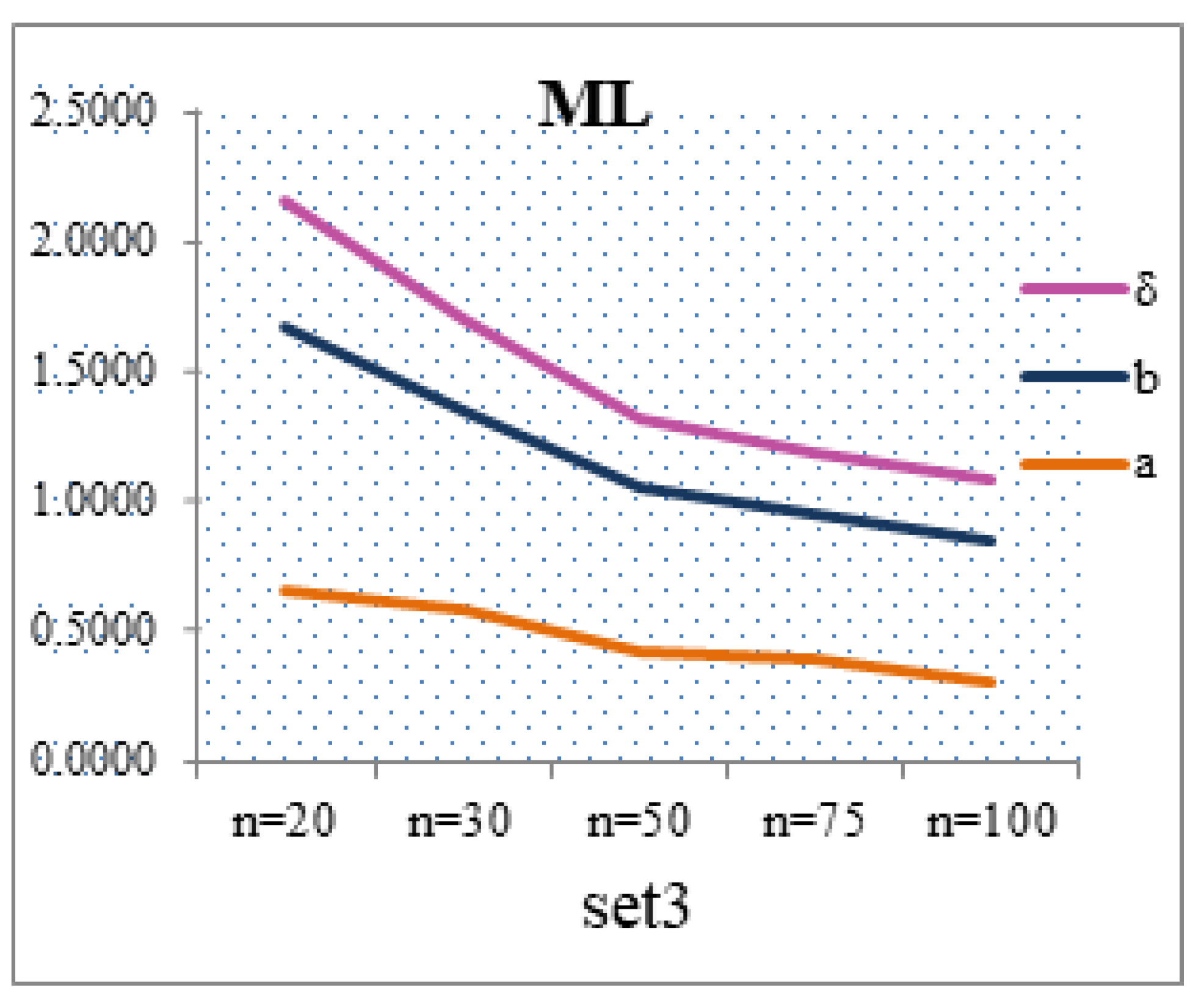
The parameter estimators of the UEHLPS class of distributions based on ML, MPS, LS, WLS, and CM are discussed in this section.

6.1. ML Estimation

Let Z 1 , , Z n be the observed values from the UEHLPS class of distributions with a set of parameters ϖ ( a , b , δ ) T . The likelihood function, say L ( ϖ ) of the UEHLPS distributions is expressed as:
L ( ϖ ) = ( 2 a b δ ) n D ( δ ) n i = 1 n z i a 1 ( 1 z i a ) b 1 ( 1 + z i a ) ( b + 1 ) D δ 1 Λ z i , a , b .
Following that, the UEHLPS distributions’ log-likelihood function, say , is shown:
= n log ( 2 a b δ ) n log D ( δ ) + ( a 1 ) i = 1 n log ( z i ) + ( b 1 ) i = 1 n log ( 1 z i a ) ( b + 1 ) i = 1 n log ( 1 + z i a ) + i = 1 n log [ D δ 1 Λ z i , a , b ] .
The components of the score vector are
U δ = n δ n D ( δ ) D ( δ ) + i = 1 n 1 Λ z i , a , b D δ 1 Λ z i , a , b D δ 1 Λ z i , a , b ,
U a = n a + i = 1 n log ( z i ) i = 1 n ( b 1 ) log ( z i ) ( z i a 1 ) i = 1 n ( b + 1 ) log ( z i ) 1 + z i a + i = 1 n D δ 1 Λ z i , a , b D δ 1 Λ z i , a , b 2 b z i a log ( z i ) ( 1 + z i a ) 2 1 z i a 1 + z i a b 1 ,
and
U b = n b + i = 1 n log ( 1 z i a ) i = 1 n log ( 1 + z i a ) i = 1 n D δ 1 Λ z i , a , b D δ 1 Λ z i , a , b 1 z i a 1 + z i a b log 1 z i a 1 + z i a .
Setting the nonlinear system of equations U δ = U a = U b = 0 and solving them simultaneously yields the ML estimator (MLE), say a ^ 1 , b ^ 1 , and δ ^ 1 . Use of nonlinear optimization techniques, such as the quasi-Newton algorithm, to numerically maximize , is typically more practical for solving these equations.

6.2. Maximum Product of Spacings Estimation

In the case of continuous univariate distributions, the MPS estimation approach was suggested by Cheng and Amin [34] and supported by Ranneby [35] as an alternative to the ML method. It was shown that the MPS technique yields consistent and asymptotically successful estimators for a number of distributions, including a three-parameter gamma, lognormal, or Weibull, where the ML method fails due to the likelihood’s unboundedness.
In this method, an ordered sample z ( 1 ) , , z ( n ) of size n is drawn from a population having UEHLPS distributions given by (6). The uniform spacings may be determined as follows,
Ξ * ( ϖ ) = 1 n + 1 log i = 1 n + 1 Y ( i ) ,
Y ( i ) = Y ( 1 ) = H ( z ( 1 ) ; ϖ ) Y ( i ) = H ( z ( i ) ; ϖ ) H ( z ( i 1 ) ; ϖ ) i = 2 , , n Y ( n + 1 ) = 1 H ( z ( n ) ; ϖ )
where Ξ i * ( ϖ ) = H z ( i ) ; ϖ H z ( i 1 ) ; ϖ , i = 1 , 2 , , n + 1 ,
H z ( 0 ) ; ϖ = 0 , H z ( n + 1 ) ; ϖ = 1 , i = 1 n + 1 Ξ i * ( ϖ ) = 1 .
The MPS estimators of ϖ = ( δ , a , b ) T , represented by ϖ = ( δ ^ 2 , a ^ 2 , b ^ 2 ) T , can be obtained by maximizing the geometric mean of the spacings
Ξ * ( ϖ ) = 1 n + 1 i = 1 n + 1 log 1 D ( δ ) D δ 1 Λ z ( i ) , a , b 1 D ( δ ) D δ 1 Λ z ( i 1 ) , a , b ,
with respect to a , b and δ . However, the obtained estimators a ^ 2 , b ^ 2 , and δ ^ 2 , cannot be solved analytically, so numerical technique will be employed using nonlinear optimization algorithms.

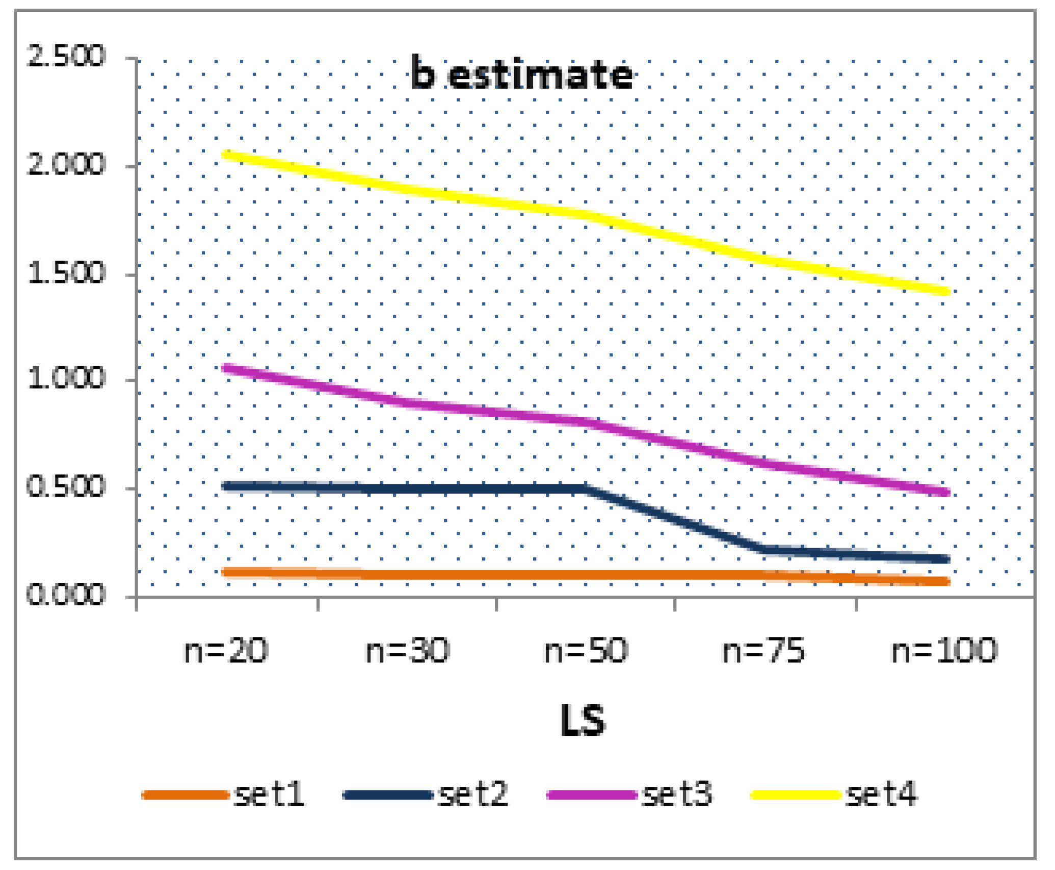
6.3. LS and WLS Estimation

Let z ( 1 ) , , z ( n ) an ordered sample of size n is drawn from UEHLPS distributions (6). The LS estimators, say a ^ 3 , b ^ 3 , and δ ^ 3 , are obtained by minimizing the following function:
Q ( ϖ ) = i = 1 n A i 1 D ( δ ) D δ 1 Λ z ( i ) , a , b i n + 1 2 ,
with respect to ϖ ( a , b , δ ) T , where, i = 1 , 2 , , n . Hence, we obtain a ^ 3 , b ^ 3 , and δ ^ 3 by setting A i = 1 in (29). Similarly, the WLS estimators, say a ^ 4 , b ^ 4 , and δ ^ 4 , are produced by minimizing (29) with respect to a , b and δ where A i = ( n + 2 ) ( n + 1 ) 2 i ( n i + 1 ) , i = 1 , 2 , , n . However, the estimators a ^ 4 , b ^ 4 , and δ ^ 4 , cannot be solved analytically so the numerical method will be used with a nonlinear optimization technique.

6.4. Cramér–von Mises Estimation

Let z ( 1 ) , , z ( n ) an ordered sample of size n drawn from UEHLPS distributions (6). The CV estimators a ^ 5 , b ^ 5 , and δ ^ 5 , of a , b and δ , respectively, are obtained by minimizing the following function:
C ( ϖ ) = 1 12 n + i = 1 n 1 D ( δ ) D δ 1 Λ z ( i ) , a , b 2 i 1 2 n 2 ,
with respect to ϖ . However, the estimators a ^ 5 , b ^ 5 , and δ ^ 5 , cannot be solved analytically so the numerical method will be used with a nonlinear optimization technique.

7. Simulation

To examine the effectiveness of the various estimators, we conducted a simulation study in this part. We evaluate the ML, LS, WLS, MPS, and CM estimates based on the mean squared errors (MSEs) and relative biases (RBs) for various sample sizes. 1000 random samples Z 1 , , Z n of sizes n = 20, 30, 50, 75, and 100 are generated from the UEHLP distribution. We take into account the following four sets of parameters: set 1 a = 0.8 , b = 0.8 , δ = 0.5 , set 2 ( a = 0.8 , b = 1.5 , δ = 0.8 ) , set 3 ( a = 2 , b = 1.5 , δ = 0.5 ) and set 4 ( a = 1.5 , b = 0.8 , δ = 0.3 ) .
The ML, LS, WLS, MPS, and CV estimates of a, b and δ are computed. Then, the MSEs and RBs of the estimates of the unknown parameters are calculated. The following findings are noted after analyzing the simulated results in Table 2 and Table 3 and Figure 6, Figure 7, Figure 8, Figure 9, Figure 10 and Figure 11.
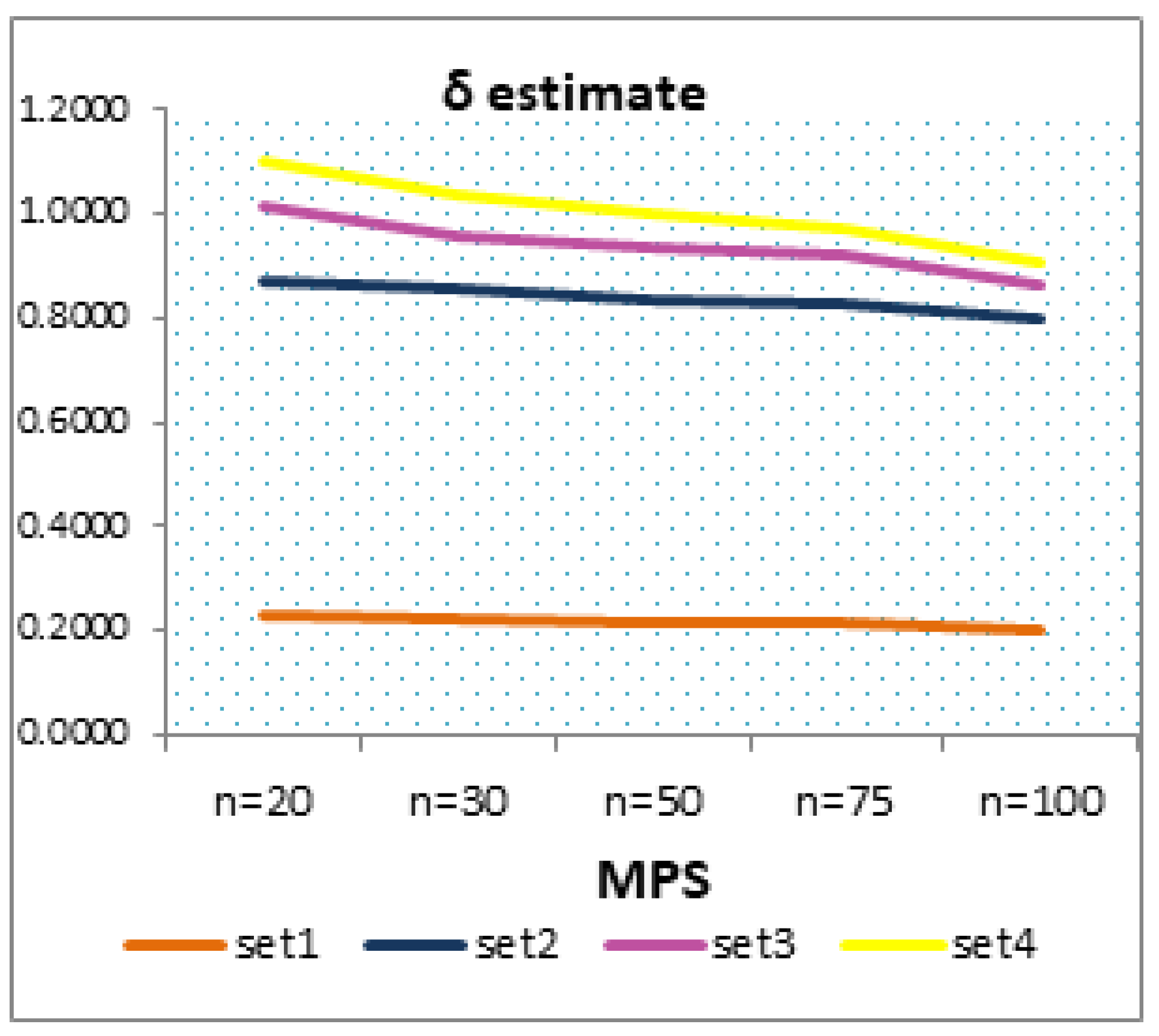
  • All of the estimates exhibit consistency properties.
  • The MSEs and RBs decrease as sample sizes increase for all sets of parameters (see Table 2 and Table 3 and Figure 8, Figure 9 and Figure 11).
  • The MSEs and RBs of the MPS estimates appear to take the least values corresponding to the other estimates for all sample sizes and all sets of parameters, based on Figure 6 and Figure 7 and Table 2 and Table 3.
  • In most cases, Set 1 is the best set for estimating the parameters corresponding to the other sets (see for example Figure 6, Figure 7, Figure 8, Figure 9, Figure 10 and Figure 11).
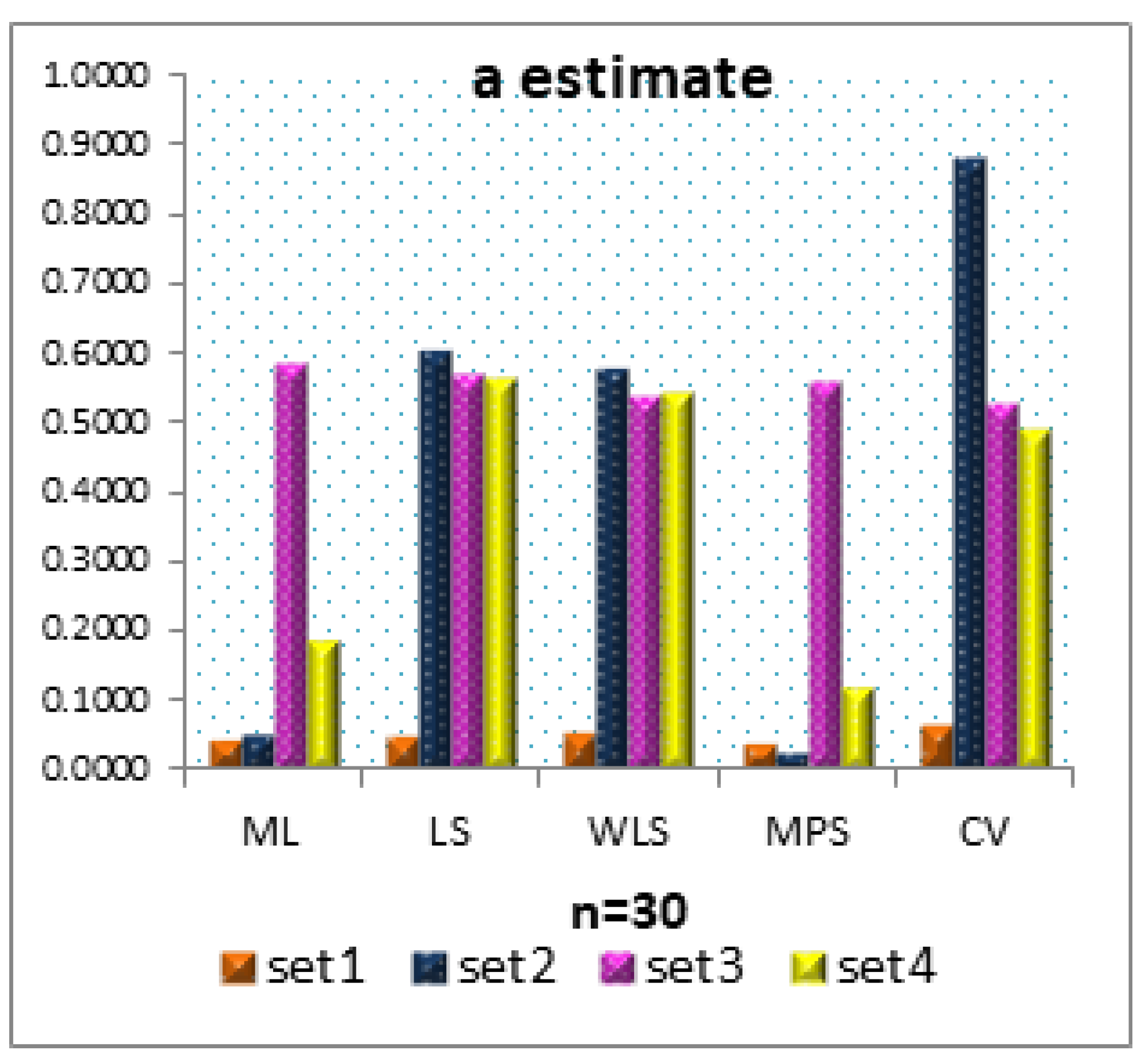
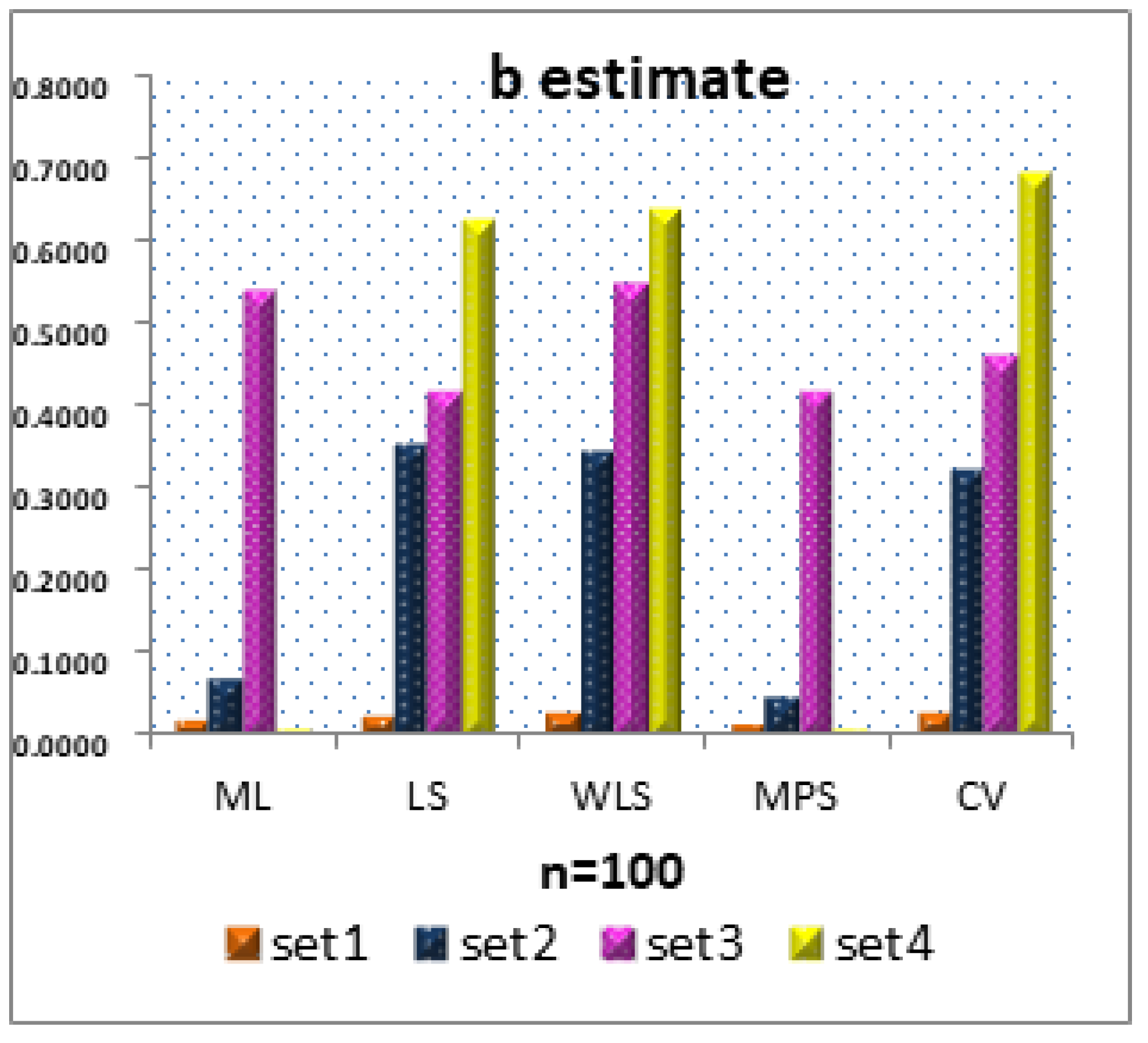
  • For a fixed value of a = 0.8 and as the value of b , δ increases, the MSEs and RBs for a and b estimates are increasing, also the MSEs and RBs for δ decreasing based on all methods for almost sample sizes (see for example Table 2).
  • For increasing value of a and as the value of b , δ decrease, the MSEs and RBs for a , b and δ estimates are decreasing based on all methods and for all sample sizes (see Table 3).
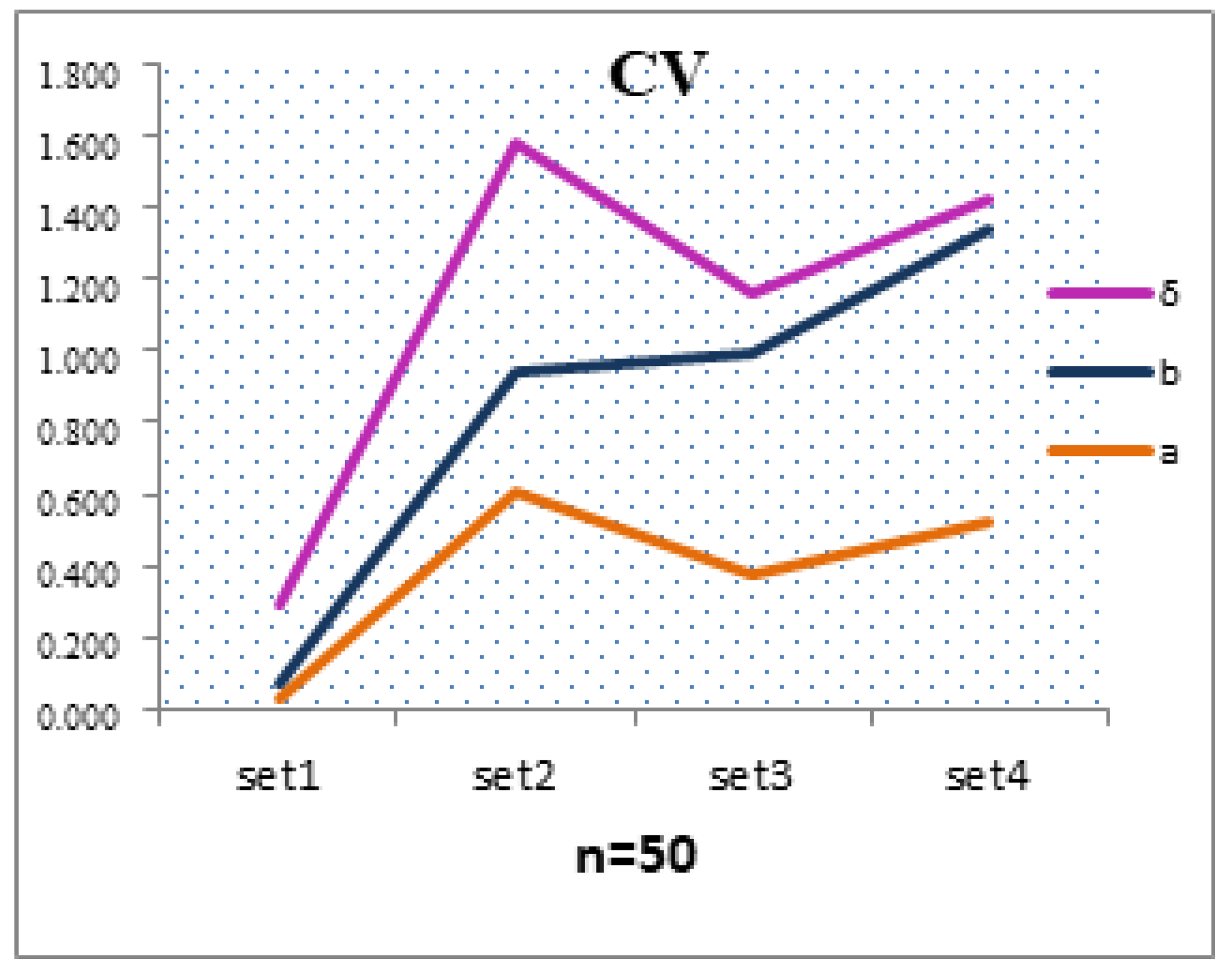
  • From Figure 6, the MSEs of the CV method for Set 1 have the smallest MSE among other sets of parameters.
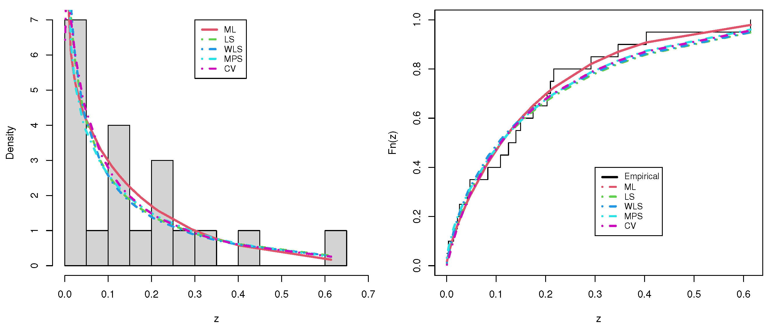
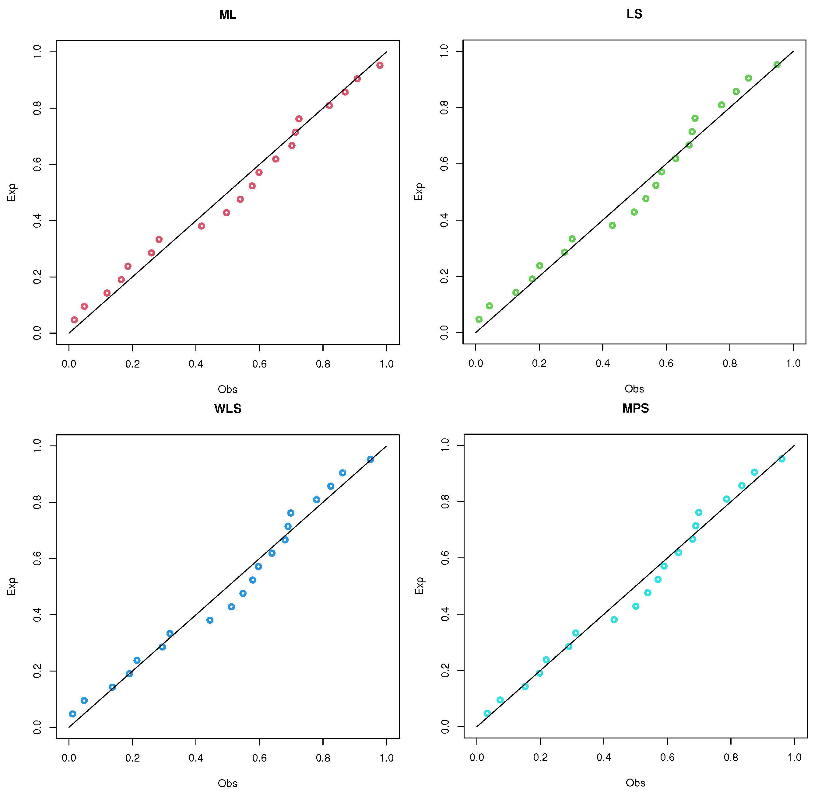
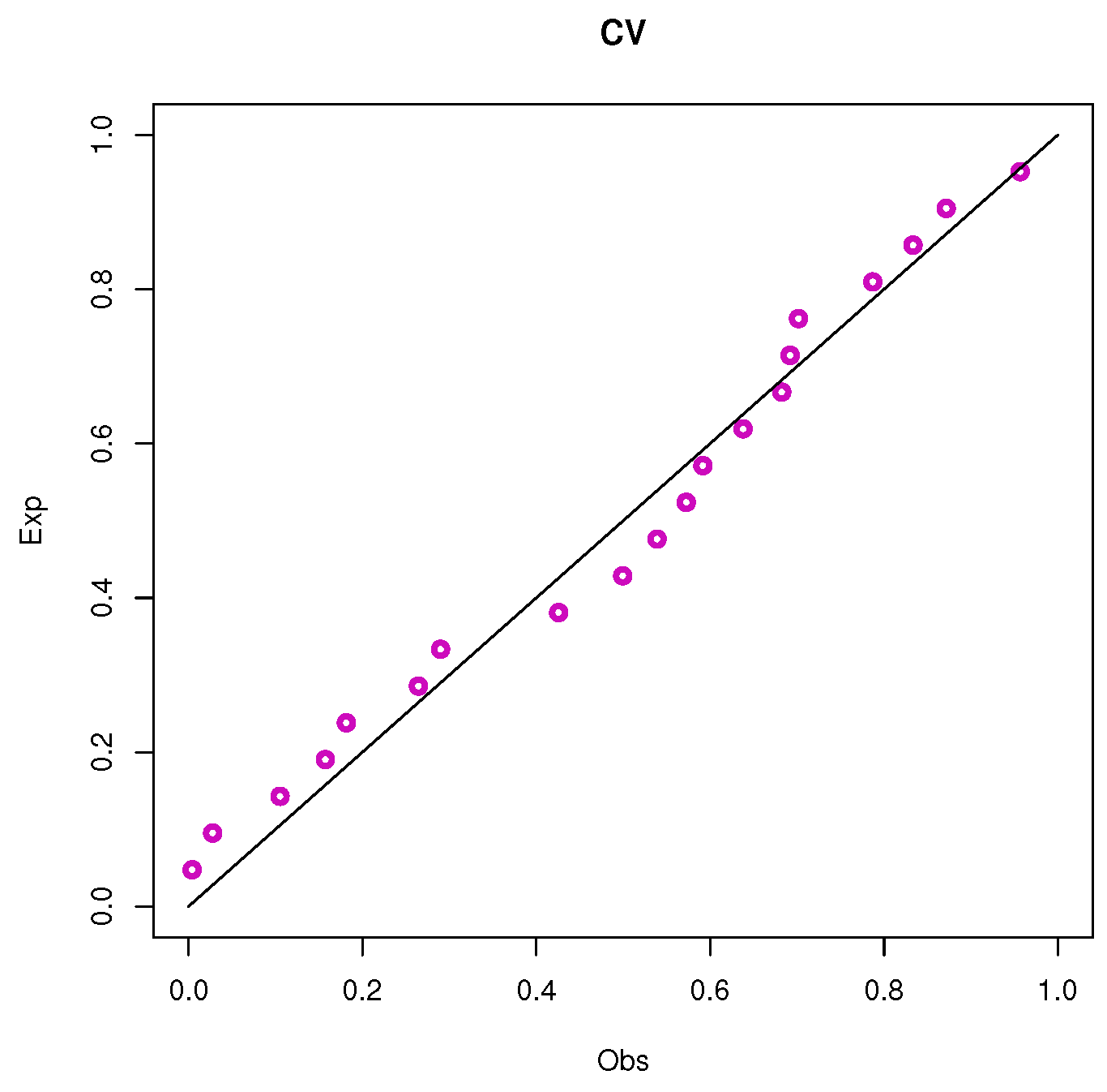
  • The estimated parameter of a is the best compared to the estimated parameters of b , δ (see Figure 10 and Figure 11).

8. Data Application

In this part, three real data examples from various scientific domains are modeled using the new UEHLP model as an example of the UEHLPS class distributions. For comparison with the UEHLP model, many distributions are recommended, such as the unit exponential Pareto (UEP) model [36], the exponential Pareto (EP) model [37], the unit-Weibull (UW) model [38], Marshall-Olkin extended Topp–Leone (MOETL) model [39], unit-Gompertz (UG) model [40], unit gamma/Gompertz (UGG) model [41], Kavya–Manoharan Kumaraswamy (KMKw) model [42], Kumaraswamy (Kw) model [43], power Topp-Leone (PTL) model [44] and type I half-logistic Topp-Leone (TIHLTL) model [45].
Four measures of goodness of fit are used, the CV, Anderson–Darling (AN-D) test, Kolmogorov–Smirnov (KOS) and the p-value is evaluated for reliable results.
The first data set includes 25 observations covering the period from 27 March 2020 to 20 April 2020 of the daily ratio of total recoveries to the total number of confirmed cases in Turkey. Accessed by https://en.wikipedia.org/wiki/COVID-19_pandemic_in_TurkeyCumulative_cases,_recoveries,_and_deaths.
The data set is: 0.0568, 0.0605, 0.0648, 0.0074, 0.0095, 0.0113, 0.015, 0.018, 0.0212, 0.0229, 0.0231, 0.127, 0.1388, 0.1476, 0.0328, 0.0385, 0.0818, 0.0955, 0.0439, 0.1099, 0.0464, 0.0483, 0.0507, 0.0515, 0.0737.
The second set of data relates to milk production. This data set includes the total milk production from 107 SINDI race cows’ first calves. The details can be found in [46]. The data set is: 0.4371, 0.4694, 0.5285, 0.5629, 0.6114, 0.6844, 0.7687, 0.0671, 0.2356, 0.3383, 0.3906, 0.4438, 0.0168, 0.4612, 0.515, 0.5553, 0.6012, 0.6768, 0.7471, 0.0609, 0.216, 0.3259, 0.3821, 0.4365, 0.4675, 0.3175, 0.3635, 0.426, 0.4576, 0.5232, 0.5627, 0.6058, 0.6789, 0.7629, 0.065, 0.2303, 0.3323, 0.3891, 0.4741, 0.5349, 0.5707, 0.6174, 0.686, 0.7804, 0.0776, 0.1546, 0.3188, 0.3751, 0.4332, 0.2361, 0.3406, 0.3945, 0.447, 0.4752, 0.535, 0.5744, 0.6196, 0.6891, 0.8147, 0.0854, 0.2605, 0.3413, 0.4049, 0.4517, 0.48, 0.5394, 0.577, 0.622, 0.6907, 0.8492, 0.1131, 0.2681, 0.348, 0.4111, 0.453, 0.4823, 0.5447, 0.5853, 0.6465, 0.6927, 0.8781, 0.1167, 0.2747, 0.3598, 0.4143, 0.4553, 0.499, 0.5481, 0.5878, 0.6488, 0.7131, 0.1479, 0.3134, 0.3627, 0.4151, 0.4564, 0.5113, 0.5483, 0.5912, 0.6707, 0.7261, 0.1525, 0.514, 0.5529, 0.5941, 0.675, 0.729. The third data set is taken from [47] and is known as the failure components data; it is about the ordered failure of 20 components. The data set is: 0.2099, 0.2168, 0.2918, 9.00 × 10 4 , 0.004, 0.1404, 0.1498, 0.175, 0.0261, 0.0418, 0.0473, 0.0834, 0.1091, 0.1252, 0.2031, 0.0142, 0.0221, 0.3465, 0.4035, 0.6143.
Ten different statistical models are recommended for comparison with the UEHLP model in Table 4, Table 5 and Table 6. It is obvious that the UEHLP model, which has a high p-value, achieves the minimal value for all of the goodness of fit metrics. This shows that the UEHLP model is more appropriate and effective than utilizing the other competing models for the three suggested real-world data sets. The estimated PDF, CDF, SF, and probability-probability (PP) plots of the UEHLP model for the three suggested real-world data sets are shown in Figure 12, Figure 13 and Figure 14. Additionally, the numerical values of ML estimates and their standard errors (SEs) in Table 4, Table 5 and Table 6 are indicated.
For the proposed model, the estimated parameters, CV, AN-D, KOS, and p-value are determined using various estimation techniques and are provided in Table 7, Table 8 and Table 9 for the three real data sets, respectively. For the three proposed real-world data sets, Figure 15, Figure 16, Figure 17, Figure 18, Figure 19 and Figure 20 show the plots of the estimated PDF, CDF, and PP plots of the UEHLP model utilizing ML, LS, WLS, MPS, and CV techniques of estimation. The ML approach is the best method of estimation for the numerical values in Table 7, Table 8 and Table 9.

9. Concluding Remarks

In this study, a novel class of bounded distributions known as the unit exponentiated half logistic power series (UEHLPS) is created. This class is created by combining the power series and the unit exponentiated half logistic (UEHL) distributions. This compounding method allows for the construction of important distributions with significant physical importance in the disciplines of biology and engineering. Four new sub-models are provided. Statistical aspects of the class include formulas for the quantile function, entropy measurements, moments and incomplete moments, limiting behavior, density, and cumulative distribution functions. The parameters of one sub-model of the class are estimated using five estimation techniques. Using simulated data, we assess how well the various estimators perform. According to the simulated results, the estimates based on the MPS typically have lower accuracy measure values than the other estimates. To illustrate the usefulness of one sub-model, three real data sets from various scientific areas are used. The new model that has been developed frequently provides better fits for these data sets than the other ten competing models. Some directions can be done in future research, with an estimation based on ranked set sampling being one of the key areas [48,49,50]. Moreover, the multivariate case may be regarded as extended work [51,52].

Author Contributions

S.M.A., A.S.H., M.E., I.E., R.E.M. and M.S.; Methodology, S.M.A., A.S.H., M.E., I.E., R.E.M. and M.S.; Formal analysis, S.M.A., A.S.H., M.E., I.E., R.E.M. and M.S.; Writing—original draft, S.M.A., A.S.H., M.E., I.E., R.E.M. and M.S.; Writing—review & editing, S.M.A., A.S.H., M.E., I.E., R.E.M. and M.S. All authors have read and agreed to the published version of the manuscript.

Funding

Researchers supporting project number (RSP2023R464), King Saud University, Riyadh, Saudi Arabia.

Data Availability Statement

Data sets are available in the application section.

Conflicts of Interest

The authors declare no conflict of interest.

References

  1. Morais, A.L.; Barreto-Souza, W. A compound class of Weibull and power series distribution. Comput. Stat. Data Anal. 2011, 55, 1410–1425. [Google Scholar]
  2. Mahmoudi, E.; Jafari, A.A. Generalized exponential power series distributions. Comput. Stat. Data Anal. 2012, 56, 4047–4066. [Google Scholar]
  3. Silva, R.B.; Bourguignon, M.; Dias, C.R.B.; Cordeiro, G.M. The compound family of extended Weibull power series distributions. Comput. Stat. Data Anal. 2013, 58, 352–367. [Google Scholar]
  4. Jafari, A.A.; Tahmasebi, S. Gompertz-power series distributions. Commun. Stat. Theory Methods 2016, 45, 3761–3781. [Google Scholar] [CrossRef] [Green Version]
  5. Elbatal, I.; Zayedm, M.; Rasekhi, M.; Butt, N.S. The Exponential Pareto Power Series Distribution: Theory and Applications. Pak. J. Stat. Oper. Res. 2017, 13, 603–615. [Google Scholar]
  6. Silva, R.B.; Corderio, G.M. The Burr XII power series distributions: A new compounding family. Braz. J. Probab. Stat. 2015, 29, 565–589. [Google Scholar]
  7. Oluyede, B.; Mdlongwa, P.; Makubate, B.; Huang, S. The Burr–Weibull power series class of distributions. Austrian J. Stat. 2018, 48, 1–13. [Google Scholar] [CrossRef] [Green Version]
  8. Alizadeh, M.; Bagheri, S.F.; Bahrami-Samani, E.; Ghobadi, S.; Nadarajah, S. Exponentiated power Lindley power series class of distributions: Theory and applications. Commun.-Stat.-Simul. Comput. 2018, 47, 2499–2531. [Google Scholar]
  9. Alkarni, S.H. Generalized inverse Lindley power series distributions: Modeling and simulation. J. Nonlinear Sci. Appl. 2019, 12, 799–815. [Google Scholar]
  10. Makubate, B.; Gabanakgosi, M.; Chipepa, F.; Oluyede, B. A new Lindley–Burr XII power series distribution: Model, properties and applications. Heliyon 2021, 7, e07146. [Google Scholar]
  11. Rivera, P.A.; Calderín-Ojeda, E.; Gallardo, D.I.; Gómez, H.W. A Compound Class of the Inverse Gamma and Power Series Distributions. Symmetry 2021, 13, 1328. [Google Scholar] [CrossRef]
  12. Hassan, A.S.; Almetwally, E.M.; Gamoura, S.C.; Metwally, A.S.M. Inverse exponentiated Lomax power series distribution: Model, estimation and application. J. Math. 2022, 2022, 1998653. [Google Scholar] [CrossRef]
  13. Flores, J.; Borges, P.; Cancho, V.G.; Louzada, F. The complementary exponential power series distribution. Braz. J. Probab. Stat. 2013, 27, 565–584. [Google Scholar]
  14. Hassan, A.S.; Assar, M.S.; Ali, K.A. Complementary Poisson–Lindley class of distributions. Int. J. Adv. Stat. Probab. 2015, 3, 146–160. [Google Scholar]
  15. Bagheri, S.F.; Samani, E.B.; Ganjali, M. The generalized modified Weibull power series distribution: Theory and applications. Comput. Stat. Data Anal. 2016, 94, 136–160. [Google Scholar]
  16. Hassan, A.S.; Abd-Elfattah, A.M.; Hussein, A.M. The complementary exponentiated inverted Weibull power series family of distribution and its applications. Br. J. Math. Comput. Sci. 2016, 13, 1–20. [Google Scholar] [CrossRef]
  17. Oluyede, B.O.; Mashabe, B.; Fagbamigbe, A.; Makubate, B.; Wanduku, D. The exponentiated generalized power series family of distributions: Theory, properties and applications. Heliyon 2020, 6, e04653. [Google Scholar] [CrossRef]
  18. Hassan, A.S.; Assar, S.M. A new class of power function distribution: Properties and applications. Ann. Data Sci. 2021, 8, 205–225. [Google Scholar]
  19. Papke, L.E.; Wooldridge, J.M. Econometric methods for fractional response variables with an application to 401(K) plan participation rates. J. Appl. Econom. 1996, 11, 619–632. [Google Scholar]
  20. Jiang, R. A new bathtub curve model with finite support. Reliab. Eng. Syst. Saf. 2013, 119, 44–51. [Google Scholar]
  21. Dedecius, K.; Ettler, P. Overview of bounded support distributions and methods for Bayesian treatment of industrial data. In Proceedings of the 10th International Conference on Informatics in Control, Automation and Robotics (ICINCO), Reykjavik, Iceland, 29–31 July 2013; pp. 380–387. [Google Scholar]
  22. Genc, A.I. Estimation of P(X > Y) with Topp-Leone distribution. J. Stat. Comput. Simul. 2013, 83, 326–339. [Google Scholar] [CrossRef]
  23. Almetwally, E.M.; Jawa, T.M.; Sayed, A.N.; Park, C.; Zakarya, M.; Dey, S. Analysis of unit-Weibull based on progressive type-II censored with optimal scheme. J. Alex. Eng. J. 2023, 63, 321–338. [Google Scholar]
  24. Alrumayh, A.; Weera, W.; Khogeer, H.A.; Almetwally, E.M. Optimal analysis of adaptive type-II progressive censored for new unit-Lindley model. J. King Saud Uni. Sci. 2023, 35, 102462. [Google Scholar]
  25. Hassan, A.S.; Fayomi, A.; Algarni, A.; Almetwally, E.M. Bayesian and non-Bayesian inference for unit exponentiated half logistic distribution with data analysis. Appl. Sci. 2022, 12, 11253. [Google Scholar] [CrossRef]
  26. Patil, G.P. Certain Properties of the Generalized Power Series Distribution. Ann. Math. Stat. 1962, 21, 179–182. [Google Scholar]
  27. Patil, G.P. On homogeneity and combined estimation for the generalized power series distribution and certain applications. Biometrics 1962, 18, 365–374. [Google Scholar] [CrossRef]
  28. Patil, G.P. Minimum variance unbiased estimation and certain problems of additive number theory. Ann. Math. Stat. 1963, 34, 1050–1056. [Google Scholar] [CrossRef]
  29. Zamanzade, E.; Mahdizadeh, M. Goodness of fit tests for Rayleigh distribution based on Phi-divergence. Rev. Colomb. EstadíStica 2017, 40, 279–290. [Google Scholar]
  30. Mahdizadeh, M.; Zamanzade, E. A comprehensive study of lognormality tests. Electron. J. Appl. Stat. Anal. 2017, 10, 349–373. [Google Scholar]
  31. Mahdizadeh, M.; Zamanzade, E. New goodness of fit tests for the Cauchy distribution. J. Appl. Stat. 2017, 44, 1106–1121. [Google Scholar] [CrossRef]
  32. Mahdizadeh, M.; Zamanzade, E. Goodness-of-fit testing for the Cauchy distribution with application to financial modeling. J. King Saud-Univ.-Sci. 2019, 31, 1167–1174. [Google Scholar]
  33. Gradshteyn, I.S.; Ryzhik, I.M. Table of Integrals, Series and Products; Academic Press: San Diego, CA, USA, 2000. [Google Scholar]
  34. Cheng, R.C.H.; Amin, N.A.K. Product-of-Spacings Estimation with Applications to the Lognormal Distribution; Math Report 79-1; University of Wales IST: Cardiff, UK, 1979. [Google Scholar]
  35. Ranneby, B. The maximum spacing method. An estimation method related to the maximum likelihood method. Scand. J. Stat. 1984, 93–112. [Google Scholar]
  36. Haj Ahmad, H.; Almetwally, E.M.; Elgarhy, M.; Ramadan, D.A. On unit exponential pareto distribution for modeling the recovery rate of COVID-19. Processes 2023, 11, 232. [Google Scholar] [CrossRef]
  37. Al-Kadim, K.A.; Boshi, M.A. Exponential Pareto distribution. Math. Theory Model. 2013, 3, 135–146. [Google Scholar]
  38. Mazucheli, J.; Menezes, A.F.B.; Ghitany, M.E. The unit-Weibull distribution and associated inference. J. Appl. Probab. Stat. 2018, 13, 1–22. [Google Scholar]
  39. Opone, F.C.; Osemwenkhae, J.E. The transmuted Marshall-Olkin extended Topp-Leone distribution. Earthline J. Math. Sci. 2022, 9, 179–199. [Google Scholar]
  40. Mazucheli, J.; Menezes, A.F.; Dey, S. Unit-Gompertz distribution with applications. Statistica 2019, 79, 25–43. [Google Scholar]
  41. Bantan, R.A.; Jamal, F.; Chesneau, C.; Elgarhy, M. Theory and applications of the unit gamma/Gompertz distribution. Mathematics 2021, 9, 1850. [Google Scholar]
  42. Alotaibi, N.; Elbatal, I.; Shrahili, M.; Al-Moisheer, A.S.; Elgarhy, M.; Almetwally, E.M. Statistical inference for the Kavya–Manoharan Kumaraswamy model under ranked set sampling with applications. Symmetry 2023, 15, 587. [Google Scholar]
  43. Kumaraswamy, P. A generalized probability density function for double-bounded random processes. J. Hydrol. 1980, 46, 79–88. [Google Scholar]
  44. Elgarhy, M.; Hassan, A.S.; Nagy, H. Parameter estimation methods and applications of the power Topp-Leone distribution. Gazi Univ. J. Sci. 2022, 35, 731–746. [Google Scholar] [CrossRef]
  45. ZeinEldin, R.A.; Chesneau, C.; Jamal, F.; Elgarhy, M. Different estimation methods for type I half-Logistic Topp–Leone distribution. Mathematics 2019, 7, 985. [Google Scholar] [CrossRef] [Green Version]
  46. Cordeiro, G.M.; dos Santos Brito, R. The beta power distribution. Braz. J. Probab. Stat. 2012, 26, 88–112. [Google Scholar]
  47. Nigm, A.M.; Al-Hussaini, E.K.; Jaheen, Z.F. Bayesian one-sample prediction of future observations under Pareto distribution. Statistics 2003, 37, 527–536. [Google Scholar] [CrossRef]
  48. Hassan, A.S.; Elshaarawy, R.S.; Nagy, H.F. Parameter estimation of exponentiated exponential distribution under selective ranked set sampling. Stat. Transit. New Ser. 2022, 23, 37–58. [Google Scholar] [CrossRef]
  49. Nagy, H.F.; Al-Omari, A.I.; Hassan, A.S.; Alomani, G.A. Improved estimation of the inverted Kumaraswamy distribution parameters based on ranked set sampling with an application to real data. Mathematics 2022, 10, 4102. [Google Scholar] [CrossRef]
  50. Hassan, A.S.; Almanjahie, I.M.; Al-Omari, A.I.; Alzoubi, L.; Nagy, H.F. Stress-strength modeling using median ranked set sampling: Estimation, simulation, and application. Mathematics 2023, 11, 318. [Google Scholar] [CrossRef]
  51. Patil, G.P. On multivariate generalized power series distribution and its application to the multinomial and negative multinomial. Indian J. Stat. Ser. A 1966, 28, 225–238. [Google Scholar]
  52. Patil, G.P. On sampling with replacement from populations with multiple characters. Indian J. Stat. Ser. B 1968, 30, 355–366. [Google Scholar]
Figure 1. A complete visual description of the paper.
Symmetry 15 00714 g001
Figure 2. The UEHLP density and HF for different values.
Symmetry 15 00714 g002
Figure 3. The UEHLL density and HF for different values.
Symmetry 15 00714 g003
Figure 4. The UEHLG density and HF for different values.
Symmetry 15 00714 g004
Figure 5. The UEHLB density and HF for different values.
Symmetry 15 00714 g005
Figure 6. MSEs of a estimates for different methods for all sets.
Symmetry 15 00714 g006
Figure 7. MSEs of b estimates for different methods for all sets.
Symmetry 15 00714 g007
Figure 8. MSEs of δ ^ 2 for MPS method for all sets of parameters and all sample sizes.
Symmetry 15 00714 g008
Figure 9. RBs of b ^ 3 for LS method for all sets of parameters and all sample sizes.
Symmetry 15 00714 g009
Figure 10. MSEs of a ^ 5 , b ^ 5 , and δ ^ 5 for CV method for all sets of parameters.
Symmetry 15 00714 g010
Figure 11. MSEs of a ^ 1 , b ^ 1 , and δ ^ 1 in set 3 for all n values.
Symmetry 15 00714 g011
Figure 12. Estimated PDF, CDF, SF and PP plots of UEHLP model for the first data.
Symmetry 15 00714 g012
Figure 13. Estimated PDF, CDF, SF, and PP plots of UEHLP model for the second data.
Symmetry 15 00714 g013
Figure 14. Estimated PDF, CDF, SF, and PP plots of UEHLP model for the third data.
Symmetry 15 00714 g014
Figure 15. Estimated PDF and CDF of the UEHLP model using different estimation methods for the first data.
Symmetry 15 00714 g015
Figure 16. PP plots of the UEHLP model using different estimation methods for the first data.
Symmetry 15 00714 g016aSymmetry 15 00714 g016b
Figure 17. Estimated PDF and CDF of the UEHLP model using different estimation methods for the second data.
Symmetry 15 00714 g017
Figure 18. PP plots of the UEHLP model using different estimation methods for the second data.
Symmetry 15 00714 g018aSymmetry 15 00714 g018b
Figure 19. Estimated PDF and CDF of the UEHLP model using different estimation methods for the third data.
Symmetry 15 00714 g019
Figure 20. PP plots of the UEHLP model using different estimation methods for the third data.
Symmetry 15 00714 g020aSymmetry 15 00714 g020b
Table 1. Moment values for the UEHLP Distribution.
Measures(i)(ii)(iii)(iv)(v)(vi)(vii)
μ 1 0.4350.2810.5190.5710.6620.3250.520
μ 2 0.2850.1360.3200.4020.5060.1660.366
μ 3 0.2150.0820.2190.3120.4140.1030.287
μ 4 0.1750.0560.1610.2570.3530.0710.239
σ 2 0.0960.0570.0510.0760.0670.0610.095
α 3 0.2760.873−0.007−0.174−0.5810.652−0.077
α 4 1.772.8812.1571.8822.2882.4841.712
Table 2. MSEs and RBs of UEHLP estimates for different methods at set 1 and set 2.
nMethodsPropertiesSet 1Set 2
ab δ ab δ
20MLMSE0.0690.1110.9210.0920.4190.647
RB0.3010.1850.7240.2150.0631.003
LSMSE0.0750.1110.2650.8330.4340.640
RB0.0420.1090.9520.7790.4011.000
WLSMSE0.0730.1240.3780.7960.4190.640
RB0.0280.1421.0330.7920.3961.000
MPSMSE0.0480.0600.2290.0480.2670.640
RB0.0320.0040.9670.0310.1631.000
CVMSE0.1180.1700.2321.4760.3510.640
RB0.1310.2390.9531.0640.3431.000
30MLMSE0.0450.0620.6280.0540.1710.641
RB0.0170.1470.8500.1780.0051.000
LSMSE0.0500.0680.2350.6050.4040.640
RB0.0460.1050.9650.7460.4011.000
WLSMSE0.0520.0750.3260.5760.3890.640
RB0.0200.1321.0230.7670.3951.000
MPSMSE0.0380.0350.2220.0280.1600.640
RB0.0120.0010.9610.0420.1560.998
CVMSE0.0630.0930.2290.8780.3450.640
RB0.0270.1890.9720.9150.3631.000
50MLMSE0.0230.0350.3770.0340.1020.640
RB0.0240.1200.8580.1570.1310.985
LSMSE0.0250.0390.2400.4840.3780.635
RB0.0680.1040.9770.7530.3960.999
WLSMSE0.0240.0440.3090.4790.3690.640
RB0.0620.1341.1170.7700.3930.994
MPSMSE0.0200.0210.2140.0190.0880.623
RB0.1150.0270.9560.0650.0220.994
CVMSE0.0260.0480.2140.6040.3410.632
RB0.0300.1510.9840.8490.3740.800
75MLMSE0.0180.0250.2970.0270.0830.640
RB0.0340.1040.8940.4820.5670.969
LSMSE0.0190.0290.2460.4180.3670.632
RB0.0640.1010.9890.1480.1260.990
WLSMSE0.0180.0360.3000.4240.3590.639
RB0.0540.1291.0810.7520.3950.991
MPSMSE0.0140.0160.2120.0160.0600.612
RB0.1020.0340.9560.0790.0460.715
CVMSE0.0190.0350.2100.4860.3420.626
RB0.0360.1350.9900.7930.3800.729
100MLMSE0.01530.0180.2300.0210.0690.626
RB0.0490.0930.9130.1190.5670.799
LSMSE0.0140.0220.2460.3940.3510.626
RB0.0740.0940.9880.7260.3990.952
WLSMSE0.0140.0260.2740.3990.3450.632
RB0.0620.1151.0410.7420.3970.984
MPSMSE0.0110.0130.2000.0130.0490.600
RB0.1020.0360.9480.0790.0560.701
CVMSE0.0130.0260.2020.4420.3220.614
RB0.0550.1170.9900.7720.3890.716
Table 3. MSEs and RBs of UEHLP estimates for different methods at set 3 and set 4.
nMethodsPropertiesSet 3Set 4
ab δ ab δ
20MLMSE0.6611.0120.4800.3110.0780.302
RB0.1550.5520.8620.1721.0001.044
LSMSE0.7360.6370.1640.6060.9340.090
RB0.2550.3920.7560.4771.0001.013
WLSMSE0.6750.6610.1740.5830.9400.090
RB0.2440.4110.7490.4721.0281.001
MPSMSE0.6580.5050.1480.1790.0520.083
RB0.3290.3320.6490.0280.1160.994
CVMSE0.8910.9520.1710.5220.9970.090
RB0.3180.5210.7350.4131.2270.995
30MLMSE0.5840.7680.3540.1870.0420.175
RB0.3120.5040.8080.1240.0351.039
LSMSE0.5670.5590.1640.5610.8060.090
RB0.2750.3970.7340.4800.9960.997
WLSMSE0.5360.7420.3930.5450.8230.090
RB0.2610.4840.7230.4741.0191.001
MPSMSE0.5780.4700.1040.1230.0350.080
RB0.3100.3560.5790.0230.1020.983
CVMSE0.5280.7400.1650.4900.9320.086
RB0.2070.4780.7270.4011.1420.999
50MLMSE0.4210.6300.2680.0910.0220.141
RB0.2770.4820.7510.0790.0051.001
LSMSE0.4230.5050.1610.5650.6980.090
RB0.2680.3110.7220.4880.9651.000
WLSMSE0.4110.7550.3650.5490.7120.090
RB0.2370.4180.5430.4830.9861.001
MPSMSE0.3640.4400.1000.0660.0220.063
RB0.3060.3100.4820.0110.0960.963
CVMSE0.3790.6190.1630.5210.8150.090
RB0.1260.4620.7140.3661.0490.997
75MLMSE0.4010.5520.2410.0620.0140.106
RB0.2620.4030.6580.0730.0030.994
LSMSE0.4170.4230.1570.5560.6760.090
RB0.2440.3920.7170.4820.9530.996
WLSMSE0.4040.6990.3510.5420.6880.090
RB0.2160.3130.4620.4810.9711.000
MPSMSE0.3590.4250.0960.0480.0110.053
RB0.2070.3040.3810.0020.0810.943
CVMSE0.3740.4820.1570.5160.7520.080
RB0.1110.4220.6740.3451.0290.990
100MLMSE0.3110.5370.2380.0420.0100.093
RB0.2590.3630.5650.0540.0020.988
LSMSE0.3700.4160.1430.5440.6280.090
RB0.2210.3090.6670.4750.9420.989
WLSMSE0.3140.5500.3400.5320.6380.088
RB0.2050.2390.3740.4710.9661.000
MPSMSE0.3080.4160.0600.0380.0100.043
RB0.1950.2350.3690.0010.0770.934
CVMSE0.3410.4590.1450.5010.6820.070
RB0.1020.4100.5690.2850.9940.970
Table 4. ML estimate and SE for the first data, along with certain goodness-of-fit measures.
ModelsML Estimates and SEsCVAN-DKOSp-Value
UEHLP( a , b , δ )1.310
(2.530)
19.067
(24.459)
2.447 × 10 5
(19.476)
0.0270.2090.0800.997
UEP( α , β , λ )1.342
(0.209)
0.115
(0.054)
2.063
(1.069)
0.0300.2290.1010.941
EP( α , β , λ )1.432
(0.224)
0.117
(0.909)
2.501
(27.807)
0.0300.2310.1030.930
UW( α , β )0.006
(0.003)
4.160
(0.418)
0.0650.3860.1360.692
MOETL( α , β )0.006
(0.005)
2.066
(0.298)
0.0560.3480.1060.915
UGG( α , β , λ )1.288
(0.283)
29.959
(14.070)
0.806
(0.400)
0.0390.2550.2190.156
UG( α , β )0.017
(0.013)
1.146
(0.180)
0.1240.7260.1600.493
KMKw( α , β )1.552
(0.245)
55.323
(37.219)
0.0290.2130.1020.956
Kw( α , β )1.416
(0.230)
50.934
(31.330)
0.0280.2110.1020.957
PTL( α , β )0.034
(0.022)
89.748
(111.173)
0.4227.5070.2950.026
TIHLTL( α , β )1.206
(0.221)
18.050
(8.231)
0.0330.2540.1030.955
Table 5. ML estimate and SE for the second data, along with certain goodness-of-fit measures.
ModelsML Estimates and SEsCVAN-DKOSp-Value
UEHLP( a , b , δ )1.699
(0.322)
2.554
(0.332)
2.701
(1.037)
0.0760.4470.0540.918
UEP( α , β , λ )1.209
(0.087)
1.124
(1.018)
0.843
(0.415)
0.1090.6520.0790.521
EP( α , β , λ )2.601
(0.210)
0.637
(6.204)
1.662
(42.140)
0.2321.5240.0830.449
UW( α , β )0.985
(0.102)
1.562
(0.106)
0.3962.4240.1210.089
MOETL( α , β )1.054
(0.348)
2.023
(0.412)
0.2251.4260.0970.268
UGG( α , β , λ )4.158
(1.059)
5.238
(1.603)
0.427
(0.139)
0.2201.4380.1070.175
UG( α , β )2.119
(0.868)
0.388
(0.115)
0.5213.0950.1840.002
KMKw( α , β )2.403
(0.237)
2.923
(0.548)
0.2461.5060.0860.409
Kw( α , β )2.195
(0.222)
3.436
(0.582)
0.1791.1100.0760.563
PTL( α , β )0.912
(0.380)
2.377
(1.471)
0.1981.5130.0980.251
TIHLTL( α , β )2.045
(0.271)
1.582
(0.191)
0.1230.7890.0770.546
Table 6. ML estimate and SE for the third data, along with certain goodness-of-fit measures.
ModelsML Estimates and SEsCVAN-DKOSp-Value
UEHLP( a , b , δ )0.689
(0.336)
2.531
(0.777)
1.542
(2.757)
0.0260.1570.0920.992
UEP( α , β , λ )0.729
(0.127)
0.376
(0.498)
1.536
(1.763)
0.0270.1650.0930.989
EP( α , β , λ )0.900
(0.165)
0.265
(0.759)
1.627
(0.433)
0.0430.2420.1190.907
UW( α , β )0.160
(0.071)
1.727
(0.288)
0.0570.3300.1320.833
MOETL( α , β )0.352
(0.254)
0.835
(0.274)
0.0490.2790.1100.949
UGG( α , β , λ )1.343
(1.071)
3.852
(2.309)
0.435
(0.449)
0.0400.2270.1570.651
UG( α , β )0.772
(0.279)
0.596
(0.120)
0.0430.2420.1190.907
KMKw( α , β )0.839
(0.185)
2.966
(1.248)
0.0380.2160.1160.951
Kw( α , β )0.764
(0.175)
3.434
(1.311)
0.0300.1760.1030.984
PTL( α , β )0.181
(0.236)
5.825
(12.319)
0.0440.2580.1120.965
TIHLTL( α , β )0.603
(0.171)
2.134
(0.634)
0.0270.1610.0930.991
Table 7. Estimated parameters with the goodness of fit measures by different estimation methods for the first data.
MethodsML Estimates and SEsCVAN-DKOSp-Value
ab δ
ML1.3119.0672.447 × 10 5 0.0270.2090.0800.997
LS0.2844.32230.4460.0720.4930.0300.970
WLS0.2514.32047.3220.0690.4490.0910.909
MPS0.89910.9962.5310.0300.2310.0030.996
CV0.2544.45253.3280.0460.3950.0320.968
Table 8. Estimated parameters with the goodness of fit measures by different estimation methods for the second data.
MethodsML Estimates and SEsCVAN-DKOSp-Value
ab δ
ML1.6992.5542.7010.0760.4470.0540.918
LS1.8982.7392.4540.1330.8140.1970.803
WLS1.8232.6712.5720.1250.7700.1610.839
MPS1.5582.3552.8690.1050.7010.1100.890
CV1.9442.8132.4160.1410.8640.2230.777
Table 9. Estimated parameters with the goodness of fit measures by different estimation methods for the third data.
MethodsML Estimates and SEsCVAN-DKOSp-Value
ab δ
ML0.6892.5311.5420.0260.1570.0920.992
LS0.1261.71520.5980.0520.2990.0290.971
WLS0.1011.69627.6480.0530.3090.0350.965
MPS0.4711.9592.6350.0400.2530.0130.987
CV0.0701.81773.6010.0630.3620.0190.981
Disclaimer/Publisher’s Note: The statements, opinions and data contained in all publications are solely those of the individual author(s) and contributor(s) and not of MDPI and/or the editor(s). MDPI and/or the editor(s) disclaim responsibility for any injury to people or property resulting from any ideas, methods, instructions or products referred to in the content.

