Relativistic Fermion and Boson Fields: Bose-Einstein Condensate as a Time Crystal

Abstract

In a basis of the space-time coordinate frame four quaternions discovered by Hamilton can be used. For subsequent reproduction of the coordinate frame these four quaternions are expanded to four 4 × 4 matrices with real-valued matrix coefficients −0 and 1. This group set is isomorphic to the SU(2) group. Such a matrix basis introduces extra six degrees of freedom of matter motion in space-time. There are three rotations about three space axes and three boosts along these axes. Next one declares the differential generating operators acting on the energy-momentum density tensor written in the above quaternion basis. The subsequent actions of this operator together with its transposed one on the above tensor lead to the emergence of the gravitomagnetic equations that are like the Maxwell equations. Wave equations extracted from the gravitomagnetic ones describe the propagation of energy density waves and their vortices through space. The Dirac equations and their reduction to two equations with real-valued functions, the quantum Hamilton-Jacobi equations and the continuity equations, are considered. The Klein-Gordon equations arising on the mass shell hints to the alternation of the paired fermion fields and boson ones. As an example, a Feynman diagram of an electron–positron time crystal is illustrated.

1. Introduction

Four-dimensional space-time has 10 degrees of freedom. Namely, there are four translations along the spatio-temporal coordinate axes, three rotations about the spatial coordinate axes, and three boosts along these axes. Here we do not consider the extra degrees of freedom coming from the weak and strong interactions but limit itself by the gravitomagnetic ones only.

There is an amazing compatibility between the coordinate framework of 4D spacetime and the quaternions, $\mathbf{1},\mathbf{i},\mathbf{j},\mathbf{k}$ (${\mathbf{i}}^{\mathbf{2}}={\mathbf{j}}^{\mathbf{2}}={\mathbf{k}}^{\mathbf{2}}=\mathbf{ijk}=-\mathbf{1}$) described for the first time by William Rowan Hamilton [1]. However, instead of these numbers, we introduce the quaternion basis represented by four $4\times 4$ matrices with real-valued components [2,3,4,5,6,7]:

$${\eta }_0=\hspace{1em}\left(\begin{array}{cccc}1& 0& 0& 0\\ 0& 1& 0& 0\\ 0& 0& 1& 0\\ 0& 0& 0& 1\end{array}\right),\hspace{1em}{\eta }_z=\hspace{1em}\left(\begin{array}{cccc}0& 0& 0& -1\\ 0& 0& 1& 0\\ 0& -1& 0& 0\\ 1& 0& 0& 0\end{array}\right),$$

$${\eta }_x=\hspace{1em}\left(\begin{array}{cccc}0& -1& 0& 0\\ 1& 0& 0& 0\\ 0& 0& 0& 1\\ 0& 0& -1& 0\end{array}\right),\hspace{1em}{\eta }_y=\hspace{1em}\left(\begin{array}{cccc}0& 0& -1& 0\\ 0& 0& 0& -1\\ 1& 0& 0& 0\\ 0& 1& 0& 0\end{array}\right).$$

(1)

These four $4\times 4$-matrices, ${\eta }_0$, ${\eta }_x$, ${\eta }_y$, ${\eta }_z$, are isomorphic to four $2\times 2$ matrices ${\sigma }_0$, ${\sigma }_x$, ${\sigma }_y$, ${\sigma }_z$ [6,8,9,10,11]. The latter matrices belonging to the group SU(2) are the main elements used by Roger Penrose at formulations of his twistor theory [12,13,14,15]. This theory was developed to combine the quantum mechanics and the relativity theory in the perspective to obtain the quantum gravity theory [16]. However, instead of the $2\times 2$ matrices ${\sigma }_0$, ${\sigma }_x$, ${\sigma }_y$, ${\sigma }_z$, among which the matrix ${\sigma }_y$ contains the imaginary units, we use $4\times 4$ matrices ${\eta }_0$, ${\eta }_x$, ${\eta }_y$, ${\eta }_z$, all are with real-valued components.

These matrices can perform the role of the orthogonal elements of the coordinate frame of the 4D space-time. Namely, here ${\eta }_0$ is the orthogonal element of the time axis, and ${\eta }_x$, ${\eta }_y$, ${\eta }_z$ are those of the space axes, x, y, z. The imaginary unit will be assigned a special role further.

The 4D space time is occupied by a medium in constant motion. Let us give its physical characteristics. The 3D space time contains only about 4 to 5 percent of the baryon matter [17]. Predominantly it is hydrogen and helium. The first element bears a proton and electron, but the second contains also neutrons. The helium preserves neutrons in its nucleus, since free neutrons have no infinite lifetime. As follows from the recent measurements [18], the baryon matter evolves in the flat 3D space. For this reason, we will not use curved coordinates when describing physical phenomena.

The remaining 95 percent of space-time is filled with an unknown substance called dark matter [19,20,21,22,23,24,25] and dark energy [26,27,28]. For the sake of generality, we will call this substance a dark fluid [29,30]. This fluid appears to be a Bose-Einstein superfluid condensate [21,22,25,28,31,32].

Further we consider the dark fluid as a special quantum ether disclosing its superfluid qualities such as helium at low temperatures [33,34,35,36]. There is a belief that the quantum ether is a medium in which virtual particles are constantly being created and disappearing. This medium is able to support the life of real particles accompanied by a cloud of the virtual particles shielding its naked charge. This belief stems from the everyday practice of using a powerful mathematical apparatus of the second quantization and the Feynman diagram techniques [37,38,39,40,41].

We consider the quantum ether as a medium with a torsion. It is laid in the quaternion algebra. Note that Einstein together with Cartan had an attempt to create a modification of General Relativity Theory allowing space-time to have torsion [42,43,44]. It was a short episode in Einstein’s scientific activity [45]. However, Einstein’s interests in the ether were due to the problem of linking the nature of the gravitational and electromagnetic fields into a single whole. As he wrote in his book [46]: “According to the general theory of relativity, space without ether is unthinkable; for in such a space not only will light not propagate, but also there will be no possibility of existence for the standards of space and time (measuring rods and clocks)”.

Currently, the idea of ether is not rejected by physicists. However, taking into account the claims made to the ether in the past, now it is endowed with superfluid properties [35,47,48,49]. Moreover, there is reason to believe that such an ether manifests itself as a dark matter represented by a Bose-Einstein condensate [50,51,52]. There are good reasons for this—the superfluid phase of matter pushes magnetic fields out of itself. These are manifestations of the Meissner effect [53].

The ether as a hydrodynamic-like medium poses both irrotational and solenoidal forms of motions. The latter forms can simulate particles when they are robust. Here we consider particles with the half integer spin and its antipodes—antiparticles, Their binding gives the Bose particle or a free EM photon. A cooperation of the Bose-particles is the Bose-Einstein condensate at which all Bose particles occupy the same state. It represents spontaneous symmetry breaking [54]. The lifetime of such a state grows as the size of the system grows. At this phase transition all Bose particles transferring in the Bose-Einstein condensate state obey the discrete time-translation symmetry [55]. It means that the Bose-Einstein condensate looks like a time crystal. Such crystals are time-periodic self-organized structures [56] such as the crystals of Floquet [54,57] or of Wilczek [58].

In this work we consider of the ether as a quantum superfluid medium [31] consisting of the Bose-Einstein condensate [21,25,50,51]. The Bose particles represent themselves as linked fermion and antifermion pairs. In fact, the ether is the Dirac’s sea of coupled particles and antiparticles [59,60]. The goal of this work is to consider the gravito-torsion and electromagnetic fields as a single whole through a manifestation of the superfluid ether (Einstein’s program [46]) and to link this picture with the Dirac’s fermion fields [32].

The article is organized as follows. Section 2 gives definition of the quaternion basis in which we write the energy-momentum density tensor. In Section 2.1 we are obtaining the gravitomagnetic equations (which are similar to Maxwell’s equations) and coming to the wave equations that describe propagation of massive gravitomagnetic fields. Finally we also define the Umov-Poynting vector disclosing the oscillations of these waves in the transversal plane with respect to their direction of propagation. Section 2.2 deals with acquiring the classical continuity end Hamilton-Jacobi equations at given the energy-momentum density tensor in the relativistic limit. In Section 3 we consider the Dirac and Majorana equations. Section 3.1 computes the transition from the Majorana equation to the pair of real-valued equations that are the continuity and quantum Hamilton-Jacobi equations. The latter is loaded by the relativistic quantum potential that is considered in detail in Section 3.2. Section 4 considers the superfluid vacuum as a manifestation of the Dirac’s particle-antiparticle fermion pairs. In Section 4.1 we consider the Bose-Einstein condensate as manifesting the time crystals and the ball lightning, in particular. Section 5 gives concluding remarks.

2. The Physical World in the Quaternion Basis

Under the quaternion basis we take a set of four matrices ${\eta }_0$, ${\eta }_x$, ${\eta }_y$, ${\eta }_z$, written in Equation (1). They obey the following multiplication rules:

$${\eta }_x^2={\eta }_y^2={\eta }_z^2={\eta }_z{\eta }_y{\eta }_x=-{\eta }_0.$$

(2)

All mathematical relations of the quaternion group can be obtained from these algebraic equations. Note that the orders of multiplication $\mathbf{ijk}=-\mathbf{1}$ and ${\eta }_z{\eta }_y{\eta }_x=-{\eta }_0$ are opposite to each other. The recovery of symmetry is achievable by changing the sign at any matrix ${\eta }_x$, ${\eta }_y$, or ${\eta }_z$.

First we define the generating differential operators [7,31,32,61,62]

$$\begin{array}{ccc}\hfill \mathcal{D}& =& \mathbf{i}{c}^{-1}{\partial }_t{\eta }_0+{\partial }_x{\eta }_x+{\partial }_y{\eta }_y+{\partial }_z{\eta }_z,\hfill \end{array}$$

(3)

$$\begin{array}{ccc}\hfill {\mathcal{D}}^{\mathbf{T}}& =& \mathbf{i}{c}^{-1}{\partial }_t{\eta }_0^{\mathbf{T}}+{\partial }_x{\eta }_x^{\mathbf{T}}+{\partial }_y{\eta }_y^{\mathbf{T}}+{\partial }_z{\eta }_z^{\mathbf{T}}\hfill \\ \hfill & =& \mathbf{i}{c}^{-1}{\partial }_t{\eta }_0-{\partial }_x{\eta }_x-{\partial }_y{\eta }_y-{\partial }_z{\eta }_z,\hfill \end{array}$$

(4)

needed for reproducing the space-time dynamics of a medium described by the energy-momentum density tensor. Next we will define this tensor in the quaternion basis. Here ${\partial }_t=\partial /\partial t$, ${\partial }_x=\partial /\partial x$, etc., sign $\mathbf{T}$ means the transposition, and c is the speed of light. Note that the space differential shifts are real, while the time shift is multiplied by the imaginary unit. These operators deform the space-time medium by shifting and twisting its infinitesimal volume elements. In particular, the d’Alembertian, or the wave operator, for the case of the negative metric signature $\{-1,+1,+1,+1\}$ reads

$${\mathcal{D}}^{\mathbf{T}}\mathcal{D}=\mathcal{D}{\mathcal{D}}^{\mathbf{T}}=(-c^{-2}{\partial }_t^2+{\partial }_x^2+{\partial }_y^2+{\partial }_z^2){\eta }_0=\square .$$

(5)

Before we define the energy-momentum density tensor, let us describe general signs of the medium under consideration within an unit volume $\Delta V$. These signs are a total mass M and a total charge q of the medium enclosed in a given volume. From here we may define the mass density, ${\rho }_M$ and charge density ${\rho }_q$. These densities are considered in a perspective of perfect fluids following the Euler’s and Lagrange’s formulations [63]

$$\begin{array}{ccc}\hfill {\rho }_M& =& \frac{M}{\Delta V}=\frac{m_a{N}_a+m_b{N}_b}{\Delta V}=\frac{mN}{\Delta V}=m\rho ,{\rho }_q=\frac{q}{\Delta V}=e\frac{(N_a-N_b)}{\Delta V}.\hfill \end{array}$$

(6)

Here

$$M=mN=\frac{1}{2}[(m_a+m_b)(N_a+N_b)+(m_a-m_b)(N_a-N_b)]$$

(7)

is the total mass of the medium filling this volume and N is the number of carriers of the mass m. Note that since the medium is homogeneous the unit volume $\Delta V$ covers this medium containing an enormous number of the carriers in order to have a smooth function $\rho$. The carriers are tiny particles as they are considered by Nelson in his article [64]. While $q=e(N_a-N_b)$ is its full charge, e is the unit charge equal to the absolute value of the electron charge, $N_a$ is the amount of the positive unit charges and $N_b$ is that of the negative unit charges. Note that at $\Delta V$ tending to infinity the difference $(N_a-N_b)$ goes to zero. While at small $\Delta V$ this difference can be fluctuating about zero in the value.

Let us now write down components of the energy-momentum density tensor [7]:

$$\begin{array}{ccc}\hfill ϵ& =& \gamma \left(\mathit{v}\right)({\rho }_M{c}^2-{\rho }_q\Phi )-c^{-1}{\partial }_t\varphi ,\hfill \end{array}$$

(8)

$$\begin{array}{ccc}\hfill \overrightarrow{p}& =& \gamma \left(\mathit{v}\right)({\rho }_M\overrightarrow{\mathit{v}}+{\rho }_q\overrightarrow{A})c-\nabla \varphi .\hfill \end{array}$$

(9)

Multiplication of the momentum density by the extra constant c, the light speed, is made with the aim to have equal dimensionality with the energy density. Since the electromagnetic potentials, $\Phi$ and $|\overrightarrow{A}|$, have the dimensions V (Voltage) and $\mathrm{V}·\mathrm{s}·{\mathrm{m}}^{-1}$, respectively, the both variables, ${\rho }_q\Phi$ and ${\rho }_{q}c\overrightarrow{A}$, have the dimension of [Energy/Length${}^3$]. It is equivalent to pressure.

The dimension of the expressions (8) and (9) is [Joule/meter${}^3$] that is pressure. The two rightmost terms, $c^{-1}{\partial }_t\varphi$ and $\nabla \varphi$, in these expressions contain an arbitrary variable $\varphi$, which is a free scalar field. This field does not influence the energy and the momentum densities.

The Lorentz factor, $\gamma \left(\mathit{v}\right)$, in Equations (8) and (9) reads

$$\gamma \left(\mathit{v}\right)={\displaystyle \frac{1}{\sqrt{1-{\displaystyle {\mathit{v}}^2/c^2}}}},$$

(10)

It tends to infinity when $\mathit{v}$ goes to the speed of light c.

The energy-momentum density tensor in the quaternion basis reads [7,31,32]:

$$T=\mathbf{i}ϵ{\eta }_0+p_x{\eta }_x+p_y{\eta }_y+p_z{\eta }_z-{\mathcal{D}}^{\mathbf{T}}\varphi .$$

(11)

Here ${\mathcal{D}}^{\mathbf{T}}\varphi =\mathbf{i}{c}^{-1}{\partial }_t{\eta }_0\varphi -(\nabla ·\overrightarrow{\eta })\varphi$. Further we define the Lorentz gauge condition

$$\frac{1}{4}\mathrm{trace}\mathcal{D}T=-\frac{1}{c}{\partial }_tϵ-{\partial }_x{p}_x-{\partial }_y{p}_y-{\partial }_z{p}_z-\square \varphi =0.$$

(12)

The term $\square \varphi =\mathcal{D}{\mathcal{D}}^{\mathbf{T}}\varphi$ represents a wave equation of the scalar field $\varphi$.

Let us now write out the action of the generating differential operator $\mathcal{D}$ to the energy-momentum density tensor T:

$$\begin{array}{ccc}\hfill \mathcal{D}·T& =& \left(-\frac{1}{c}\frac{\partial ϵ}{\partial t}-\frac{\partial p_x}{\partial x}-\frac{\partial p_y}{\partial y}-\frac{\partial p_z}{\partial z}-\square \varphi \right){\eta }_0\hfill \\ \hfill & +& \left(\mathbf{i}\left(\frac{\partial ϵ}{\partial x}+\frac{\partial p_x}{c\partial t}\right)-\left(\frac{\partial p_z}{\partial y}-\frac{\partial p_y}{\partial z}\right)\right){\eta }_x\hfill \\ \hfill & +& \left(\mathbf{i}\left(\frac{\partial ϵ}{\partial y}+\frac{\partial p_y}{c\partial t}\right)-\left(\frac{\partial p_x}{\partial z}-\frac{\partial p_z}{\partial x}\right)\right){\eta }_y\hfill \\ & +& \left(\mathbf{i}\left(\frac{\partial ϵ}{\partial z}+\frac{\partial p_z}{c\partial t}\right)-\left(\frac{\partial p_y}{\partial x}-\frac{\partial p_x}{\partial y}\right)\right){\eta }_z\hfill \end{array}$$

(13)

The expression under the quaternion ${\eta }_0$ when equating it to zero represents the Lorentz gauge. Only expressions at the quaternions ${\eta }_x$, ${\eta }_y$, ${\eta }_z$ remain. They do not contain terms with the free scalar field $\varphi$. These expressions represent components of the gravitomagnetic field [7,65,66,67,68,69,70] in directions of x, y, z. As a result, the above equation represents the force density tensor of this field

$${\mathbb{F}}_{\Xi \Omega }=\mathcal{D}·T=\left(\begin{array}{cccc}0& {\Omega }_x-\mathbf{i}{\Xi }_x& {\Omega }_y-\mathbf{i}{\Xi }_y& {\Omega }_z-\mathbf{i}{\Xi }_z\\ -{\Omega }_x+\mathbf{i}{\Xi }_x& 0& -{\Omega }_z+\mathbf{i}{\Xi }_z& {\Omega }_y-\mathbf{i}{\Xi }_y\\ -{\Omega }_y+\mathbf{i}{\Xi }_y& {\Omega }_z-\mathbf{i}{\Xi }_z& 0& -{\Omega }_x+\mathbf{i}{\Xi }_x\\ -{\Omega }_z+\mathbf{i}{\Xi }_z& -{\Omega }_y+\mathbf{i}{\Xi }_y& {\Omega }_x-\mathbf{i}{\Xi }_x& 0\end{array}\right).$$

(14)

Note that lengthwise in the main diagonal, there are zeros. It is a consequence of the Lorentz gauge. The solenoidal field represented by the vector

$$\overrightarrow{\Omega }=[\nabla \times \overrightarrow{p}]$$

(15)

poses real values. The conservative vector field represented by the vector

$$\overrightarrow{\Xi }=\frac{\partial }{c\partial t}\overrightarrow{p}+\nabla ϵ$$

(16)

contains the imaginary unit as a multiplier in Equation (14).

It is instructive to compare two different representation of the electromagnetic tensor. In the quaternion representation the electromagnetic tensor reads [6]:

$${\mathbb{F}}_{E,B}=\mathcal{D}·\mathbf{A}=\left(\begin{array}{cccc}0& B_x-\mathbf{i}{E}_x& B_y-\mathbf{i}{E}_y& B_z-\mathbf{i}{E}_z\\ -B_x+\mathbf{i}{E}_x& 0& -B_z+\mathbf{i}{E}_z& B_y-\mathbf{i}{E}_y\\ -B_y+\mathbf{i}{E}_y& B_z-\mathbf{i}{E}_z& 0& -B_x+\mathbf{i}{E}_x\\ -B_z+\mathbf{i}{E}_z& -B_y+\mathbf{i}{E}_y& B_x-\mathbf{i}{E}_x& 0\end{array}\right),$$

(17)

Here the vector potential $\mathbf{A}=\mathbf{i}\Phi {\eta }_0+c{A}_x{\eta }_x+c{A}_y{\eta }_y+c{A}_z{\eta }_z$ is written in the SI units and the constant c is the speed of light. In turn, adopted in the theory of electromagnetism the electromagnetic tensor looks as follows

$$F_{\mu \nu }={\partial }_{\mu }{A}_{\nu }-{\partial }_{\nu }{A}_{\mu }=\left(\begin{array}{cccc}0& -E_x& -E_y& -E_z\\ E_x& 0& -B_z& B_y\\ E_y& B_z& 0& -B_x\\ E_z& -B_y& B_x& 0\end{array}\right).$$

(18)

The electromagnetic potential in the SI inits is $A_{\mu }=(\Phi ,c{A}_x,c{A}_y,c{A}_z)$. The magnetic field $\overrightarrow{B}$ in both expressions is chosen with an extra constant multiplier c, the speed of light. Namely, $\overrightarrow{B}=c[\nabla \times \overrightarrow{A}]$. It is carried out with the aim to have equal dimension with the electric field $\overrightarrow{E}$. Accurate to the multiplier e, the electric charge, these both variables have the same dimension of force.

Externally, both tensors have a different appearance. Nevertheless, their mutual continuity is striking. It should be noted to the place that the tensor ${\mathbb{F}}_{E,B}$ is convenient for computation of passing the spin particles through the magnetic fields [2] or charged particles through the electric fields.

2.1. The Gravitomagnetic Field Equations

The gravitomagnetic fields stem from the force density tensor, ${\mathbb{F}}_{\Xi \Omega }$, after applying to it the transposed differential generating operator ${\mathcal{D}}^{\mathbf{T}}$ [31]. For that reason, first we define a 4D current of the force density that takes into account gravitation, electromagnetic, and other accompanying forces acting on the medium within the volume $\Delta V$ under consideration.

Let us define first a density distribution term of all forces acting on the medium enclosed within the unit of the volume $\Delta V$:

$$\wp =\frac{1}{4\pi }(\nabla ·\overrightarrow{F}).$$

(19)

The divisor $4\pi$ emphasizes the commonality with Maxwell’s EM equations. Here $\overrightarrow{F}$ is represented by external forces acting on the medium covered by the volume $\Delta V$ and by its internal reaction on these forces by means of pressure gradients arising in this medium [6]. Furthermore, we need to take into account shear viscosity due to friction of the medium layers induced by the pressure gradients. We will omit further this effect from our consideration. Note only that because of this neglecting we can face unwanted singularities in subsequent calculations.

Let us now define the 3D current density as $\overrightarrow{\Im }=\overrightarrow{\mathit{v}}\wp$. Here $\overrightarrow{\mathit{v}}$ is the velocity of the unit volume $\Delta V$ covering the medium under question. Finally, we define the 4D current density as follows:

$$\mathbb{J}=\mathbf{i}c\wp {\eta }_0+{\Im }_x{\eta }_x+{\Im }_y{\eta }_y+{\Im }_z{\eta }_z.$$

(20)

The continuity equation, in this case, takes the following view

$$\frac{1}{4}\mathrm{trace}\mathcal{D}\mathbb{J}-{\partial }_t\wp -{\partial }_x{\Im }_x-{\partial }_y{\Im }_y-{\partial }_z{\Im }_z=0,$$

(21)

that can be rewritten in a more evident form

$$\frac{\partial \wp }{\partial t}+(\nabla ·\overrightarrow{\Im })=0.$$

(22)

It is the continuity equation. It says that all forces acting on the medium under question are in balance among themselves. This is a manifestation of Newton’s third law.

By applying the transposed differential generating operator ${\mathcal{D}}^{\mathbf{T}}$ to the force density tensor (14) and equating it to the 4D current density $\mathbb{J}$ we come a set of gravitomagnetic equations:

$${\mathcal{D}}^{\mathbf{T}}·{\mathbb{F}}_{\Xi \Omega }={\mathcal{D}}^{\mathbf{T}}\mathcal{D}·T=\square T=\frac{4\pi }{c}\mathbb{J}.$$

(23)

By computing the product ${\mathcal{D}}^{\mathbf{T}}·{\mathbb{F}}_{\Xi \Omega }$ we obtain the following expanded equation where its terms have been sorted as coefficients under the quaternions ${\eta }_0$, ${\eta }_x$, ${\eta }_y$, ${\eta }_z$:

$$\begin{array}{ccc}\hfill {\mathcal{D}}^{\mathbf{T}}·{\mathbb{F}}_{\Xi \Omega }& =& \{-({\partial }_x{\Omega }_x+{\partial }_y{\Omega }_y+{\partial }_z{\Omega }_z)+\mathbf{i}({\partial }_x{\Xi }_x+{\partial }_y{\Xi }_y+{\partial }_z{\Xi }_z)\}{\eta }_0\hfill \\ \hfill & +& \left\{\left(-\frac{1}{c}{\partial }_t{\Xi }_x-({\partial }_y{\Omega }_z-{\partial }_z{\Omega }_y)\right)+\mathbf{i}\left(-\frac{1}{c}{\partial }_t{\Omega }_x+({\partial }_y{\Xi }_z-{\partial }_z{\Xi }_y)\right)\right\}{\eta }_x\hfill \\ \hfill & +& \left\{\left(-\frac{1}{c}{\partial }_t{\Xi }_y-({\partial }_z{\Omega }_x-{\partial }_x{\Omega }_z)\right)+\mathbf{i}\left(-\frac{1}{c}{\partial }_t{\Omega }_y+({\partial }_z{\Xi }_x-{\partial }_x{\Xi }_z)\right)\right\}{\eta }_y\hfill \\ \hfill & +& \left\{\left(-\frac{1}{c}{\partial }_t{\Xi }_z-({\partial }_x{\Omega }_y-{\partial }_y{\Omega }_x)\right)+\mathbf{i}\left(-\frac{1}{c}{\partial }_t{\Omega }_z+({\partial }_x{\Xi }_y-{\partial }_y{\Xi }_x)\right)\right\}{\eta }_z\hfill \\ & =& \frac{4\pi }{c}(\mathbf{i}c\wp {\eta }_0+{\Im }_x{\eta }_x+{\Im }_y{\eta }_y+{\Im }_z{\eta }_z).\hfill \end{array}$$

(24)

As seen from Equations (13) and (24), the operators $\mathcal{D}$ and ${\mathcal{D}}^{\mathbf{T}}$ generate curls shifting along in the space. Gathering together real and imaginary coefficients represented in the right and left parts in Equation (24) at the quaternions ${\eta }_0$, ${\eta }_x$, ${\eta }_y$, ${\eta }_z$, we obtain the following pairs of the gravitomagnetic equations

$$\begin{array}{ccc}& & (\nabla ·\overrightarrow{\Omega })=0,\hfill \end{array}$$

(25)

$$\begin{array}{ccc}& & {\displaystyle [\nabla \times \overrightarrow{\Xi }]-\frac{1}{c}\frac{\partial }{\partial t}\overrightarrow{\Omega }}=0,\hfill \end{array}$$

(26)

$$\begin{array}{ccc}& & (\nabla ·\overrightarrow{\Xi })=4\pi \wp ,\hfill \end{array}$$

(27)

$$\begin{array}{ccc}& & {\displaystyle [\nabla \times \overrightarrow{\Omega }]+\frac{1}{c}\frac{\partial }{\partial t}\overrightarrow{\Xi }=-\frac{4\pi }{c}\overrightarrow{\Im }.}\hfill \end{array}$$

(28)

The gravitomagnetic fields $(\overrightarrow{\Xi },\overrightarrow{\Omega })$ consist of the superposition of two fields—the gravito-torsion and the electromagnetic fields. The first field describes the gravitation between the material objects and their rotations about the mass center. The second field is that described by the Maxwell equations. It should be noted that the gravitomagnetic equations were first described phenomenologically by Oliver Heaviside in 1893 by ordering the Maxwell equations [65].

The first result that one can obtain from here is wave equations. In this case, it is sufficient to apply to Equation (23) the differential operator $\mathcal{D}$:

$$\mathcal{D}{\mathcal{D}}^{\mathbf{T}}·{\mathbb{F}}_{\Xi \Omega }=\frac{4\pi }{c}\mathcal{D}·\mathbb{J}$$

(29)

and we immediately obtain [7]:

$$\begin{array}{ccc}\hfill \frac{1}{c^2}\frac{{\partial }^2}{\partial t^2}\overrightarrow{\Omega }-{\nabla }^2\overrightarrow{\Omega }& =& -\frac{4\pi }{c}[\nabla \times \overrightarrow{\Im }],\hfill \end{array}$$

(30)

$$\begin{array}{ccc}\hfill \frac{1}{c^2}\frac{{\partial }^2}{\partial t^2}\overrightarrow{\Xi }-{\nabla }^2\overrightarrow{\Xi }& =& -4\pi \left(\nabla \wp +\frac{\partial }{c^2\partial t}\overrightarrow{\Im }\right).\hfill \end{array}$$

(31)

One can see that the solenoidal field, $\overrightarrow{\Omega }$, and the magnetic induction, $\overrightarrow{B}$ are isomorphic each other, and the vortex-free field, $\overrightarrow{\Xi }$, is isomorphic to the electric field $\overrightarrow{E}$. The first field comes in Equation (14) with a multiplier of 1 (real-valued unit). While the second field in Equation (14) has a multiplier i (imaginary unit). It can mean that these fields, $\overrightarrow{\Xi }$ and $\overrightarrow{\Omega }$, are orthogonal to each other. Waves of these fields propagate in a direction which is transversal to the plane where the fields $\overrightarrow{\Xi }$ and $\overrightarrow{\Omega }$ lie. This propagation is given by the Umov–Poynting vector which follows from the expression:

$$\frac{1}{2}{\mathbb{F}}_{\Xi \Omega }^{†}{\mathbb{F}}_{\Xi \Omega }=-W_0{\eta }_0-\mathbf{i}{W}_x{\eta }_x-\mathbf{i}{W}_y{\eta }_y-\mathbf{i}{W}_z{\eta }_z.$$

(32)

Here † is the sign of complex conjugation. $W_0=({\Xi }^2+{\Omega }^2)/2$, is the gravitomagnetic energy density. While $\overrightarrow{W}=[\overrightarrow{\Xi }\times \overrightarrow{\Omega }]$ is the Umov–Poynting vector, which is orthogonal to $\overrightarrow{\Xi }$ and $\overrightarrow{\Omega }$. It is a vector of the energy flux density of a gravitomagnetic field. From here it follows that the gravito-torsion and electromagnetic fields spread in an equal manner.

Let us rewrite Equations (15) and (16) for the variables $\overrightarrow{\Omega }$ and $\overrightarrow{\Xi }$ in more detail representations

$$\begin{array}{ccc}& |& \overrightarrow{\Omega }=[\nabla \times \overrightarrow{p}]=mc·\overrightarrow{\omega }+ec·\overrightarrow{B},\hfill \\ & |& \hfill \\ & |& \overrightarrow{\Xi }={\displaystyle \frac{\partial \overrightarrow{p}}{c\partial t}+\nabla ϵ}=(\underset{{\overrightarrow{\Xi }}_0}{\underbrace{\frac{\partial {\overrightarrow{p}}_0}{c\partial t}+\nabla {ϵ}_0}})+e·(\underset{\overrightarrow{E}}{\underbrace{-\frac{\partial \overrightarrow{A}}{\partial t}-\nabla \Phi }}).\hfill \end{array}$$

(33)

In the first equation $\overrightarrow{\omega }$ is the vorticity of a massive medium chump and $\overrightarrow{B}$ is the magnetic field, which is in parallel to the vorticity. In the second equation ${\overrightarrow{\Xi }}_0$ is the conservative vector field of the massive medium chump and $\overrightarrow{E}$ is the electric field. Wave Equations (30) and (31) describe propagation of the superposition of gravito-torsion and electromagnetic waves.

2.2. Computation of the Conservative (Vortex-Free) Field in the Relativistic Limit

Now let us look at the term $\overrightarrow{\Xi }$ written in Equation (16). First, we will rewrite Equations (8) and (9) in a more acceptable form for subsequent computations:

$$\begin{array}{ccc}\hfill ϵ& =& \gamma \left(\mathit{v}\right)\rho {ϵ}_{*}-c^{-1}{\partial }_t\varphi ,{ϵ}_{*}=-\frac{\partial S}{\partial t}-e\Phi ,\hfill \end{array}$$

(34)

$$\begin{array}{ccc}\hfill \overrightarrow{p}& =& \gamma \left(\mathit{v}\right)\rho {\overrightarrow{p}}_{*}c+\nabla \varphi ,{\overrightarrow{p}}_{*}=\nabla S-e\overrightarrow{A},\hfill \end{array}$$

(35)

Here we write the energy ${ϵ}_{*}$ and the momentum ${\overrightarrow{p}}_{*}$ in a pure representation. The term $\rho =N/\Delta V$ is the density of elementary carries (6) in the volume $\Delta V$ of the medium under consideration. The action S is a scalar function defining a conservative vector field. Its gradient returns this field, $\nabla S=m\overrightarrow{\mathit{v}}$. As a result, computation of the derivatives in Equation (16) reads:

$$\begin{array}{ccc}\hfill \frac{\partial \overrightarrow{p}}{c\partial t}+\nabla ϵ& =& \gamma \left(\mathit{v}\right)\frac{\partial \rho {\overrightarrow{p}}_{*}}{\partial t}+\gamma \left(\mathit{v}\right)\nabla \rho {ϵ}_{*}+\rho {\overrightarrow{p}}_{*}\frac{\partial \gamma \left(\mathit{v}\right)}{\partial t}+\rho {ϵ}_{*}\nabla \gamma \left(\mathit{v}\right)\hfill \\ & =& \gamma \left(\mathit{v}\right)(\underset{\left(\mathrm{a}\right)}{\underbrace{\frac{\partial \rho {\overrightarrow{p}}_{*}}{\partial t}+\nabla \rho {ϵ}_{*}}})+\gamma {\left(\mathit{v}\right)}^3\frac{1}{2c^2}(\underset{\left(\mathrm{b}\right)}{\underbrace{\rho {\overrightarrow{p}}_{*}\frac{\partial {\mathit{v}}^2}{\partial t}+\rho {ϵ}_{*}\nabla {\mathit{v}}^2}})\hfill \end{array}$$

(36)

As for the scalar field $\varphi$ appeared in Equations (34) and (35), its contribution to this expression is missing since the sum of $+c^{-1}{\partial }_t(\nabla \varphi )$ and $-\nabla \left(c^{-1}{\partial }_t\varphi \right)$ is zero.

In the non-relativistic limit, $\gamma \approx 1+{\mathit{v}}^2/2c^2$, the term (a) in Equation (36) dominates that of (b) because of smallness of ${\mathit{v}}^2/2c^2\ll 1$. In this limit, we deal only with the term (a) omitting (b). Taking into account the external and internal forces acting on the space-time volume under consideration, one can come to the Schrödinger equation after some computations [7].

In the relativistic limit, $\gamma \to \infty$, the picture cardinally changes. One can see that the term (a) being multiplied by $\gamma$ is negligibly small, in contrast to the term (b) multiplied by ${\gamma }^3$. For that reason we could omit the first term. However, let us consider the term (a) from another perspective [32]. We apply to this term the operators $\partial /c\partial t$ and ∇. We obtain:

$$\nabla \frac{\partial }{c\partial t}\left(\frac{\partial \rho {\overrightarrow{p}}_{*}c}{c\partial t}+\nabla \rho {ϵ}_{*}\right)=\underset{\left(\mathrm{c}\right)}{\underbrace{\frac{{\partial }^2}{c^2\partial t^2}\nabla \rho {\overrightarrow{p}}_{*}c+{\nabla }^2\frac{\partial }{c\partial t}\rho {ϵ}_{*}}}=0.$$

(37)

Note that this expression vanishes due to the infinite smallness of the term (a) with respect to the term (b). We proclaim that the Equation (37) covered by brace (c) represents the wave equation:

$$\frac{1}{c^2}\frac{{\partial }^2}{\partial t^2}\psi (\overrightarrow{r},t)-{\nabla }^2\psi (\overrightarrow{r},t)=0,$$

(38)

if and only if the following equality is true

$$\nabla \rho {\overrightarrow{p}}_{*}c=-\frac{\partial }{c\partial t}\rho {ϵ}_{*}=\psi (\overrightarrow{r},t).$$

(39)

The Lorentz gauge (12) supports it (Note that ${\overrightarrow{p}}_{*}$ in Equation (39) and $\overrightarrow{p}$ in the Lorentz gauge (12) have different dimensions. The first has the dimension [kg·m/s], the second [kg·m${}^2$/s${}^2$] due to the extra multiplier c, the speed of light, see Equation (9)). Finally we come to the following equality

$$\nabla \rho {\overrightarrow{p}}_{*}c+\frac{\partial }{c\partial t}\rho {ϵ}_{*}=\nabla \rho (\nabla S-e\overrightarrow{A})c-\frac{\partial }{c\partial t}\rho \left(\frac{\partial S}{\partial t}+e\Phi \right)=0$$

(40)

that poses the continuity equation.

Let us now consider in more detail the expression covered by the brace (b) in Equation (36). Since the term (b) is nonzero, in contrast to (a) that vanishes, we multiply (b) by its rearranged form, i.e., we perform the multiplication like $A\mathbf{c}+B\mathbf{d}$ by $A\mathbf{d}-B\mathbf{c}$. That is, $(A\mathbf{c}+B\mathbf{d})(A\mathbf{d}-B\mathbf{c})=(A^2-B^2)\mathbf{cd}-({\mathbf{c}}^2-{\mathbf{d}}^2)AB$. Here $A=\left(\rho {\overrightarrow{p}}_{*}c\right)$, $B=\left(\rho {ϵ}_{*}\right)$, $\mathbf{c}=c^{-1}{\partial }_t{\mathit{v}}^2$, and $\mathbf{d}=\nabla {\mathit{v}}^2$. We obtain

$$\begin{array}{ccc}& & \rho ·\underset{(A\mathbf{c}+B\mathbf{d})}{\underbrace{\left(\left({\overrightarrow{p}}_{*}c\right)·\frac{\partial {\mathit{v}}^2}{c\partial t}+\left({ϵ}_{*}\right)·\nabla {\mathit{v}}^2\right)}}\rho ·\underset{(A\mathbf{d}-B\mathbf{c})}{\underbrace{\left(\left({\overrightarrow{p}}_{*}c\right)·\nabla {\mathit{v}}^2-\left({ϵ}_{*}\right)·\frac{\partial {\mathit{v}}^2}{c\partial t}\right)}}\hfill \\ & =& {\rho }^2\underset{(A^2-B^2)}{\underbrace{\left[{\left({\overrightarrow{p}}_{*}c\right)}^2-{\left({ϵ}_{*}\right)}^2\right]}}\underset{\mathbf{cd}}{\underbrace{\frac{\partial {\mathit{v}}^2}{c\partial t}\nabla {\mathit{v}}^2}}-{\rho }^2\underset{({\mathbf{c}}^2-{\mathbf{d}}^2)}{\underbrace{\left[{\left(\frac{\partial {\mathit{v}}^2}{c\partial t}\right)}^2-{(\nabla {\mathit{v}}^2)}^2\right]}}\underset{AB}{\underbrace{{(\overrightarrow{p}}_{*}c)\left({ϵ}_{*}\right)}}\hfill \end{array}$$

(41)

Here the brace $(A\mathbf{c}+B\mathbf{d})$ is the copy of the expression written in Equation (36) over brace (b) and $(A\mathbf{d}-B\mathbf{c})$ is its converted form. Take note that the expression $(A\mathbf{c}+B\mathbf{d})$ is a vector, while $(A\mathbf{d}-B\mathbf{c})$ is a scalar. Their multiplication returns a vector. It is represented by $\nabla {\mathit{v}}^2$ in the first term and by ${\overrightarrow{p}}_{*}$ in the second term.

Note that multiplication of the original expression, $(A\mathbf{c}+B\mathbf{d})$, by $(A\mathbf{d}-B\mathbf{c})$ is necessary to double the fields, where these fields should be antipodes to each other. It is similar, in a way, to doubling the matrix rank for writing a new 8-by-8 matrix operator by Bocker and Frieden in [71]. Both these expressions, $(A^2-B^2)$ and $({\mathbf{c}}^2-{\mathbf{d}}^2)$, are the main parts underlying the emergence of the Dirac equation. Let us begin from the second expression, $({\mathbf{c}}^2-{\mathbf{d}}^2)=(\mathbf{c}-\mathbf{d})(\mathbf{c}+\mathbf{d})$. It is a scalar:

$$\begin{array}{ccc}\hfill & & \left(\frac{\partial {\mathit{v}}^2}{c\partial t}-|\nabla {\mathit{v}}^2|\right)\left(\frac{\partial {\mathit{v}}^2}{c\partial t}+|\nabla {\mathit{v}}^2|\right)=4{\mathit{v}}^2\left(\frac{\partial \mathit{v}}{c\partial t}-|\nabla \mathit{v}|\right)\left(\frac{\partial \mathit{v}}{c\partial t}+|\nabla \mathit{v}|\right)\hfill \\ & & =\frac{4{\mathit{v}}^2}{c^2{m}^2}\nabla \left(\frac{\partial \overrightarrow{\mathit{S}}}{\partial t}-|\nabla \overrightarrow{\mathit{S}}|c\right)\nabla \left(\frac{\partial \overrightarrow{\mathit{S}}}{\partial t}+|\nabla \overrightarrow{\mathit{S}}|c\right)=\frac{4{\mathit{v}}^2}{c^2{m}^2}\nabla (E+pc)\nabla (E-pc).\hfill \end{array}$$

(42)

Here we take into consideration that $\overrightarrow{p}=m\overrightarrow{\mathit{v}}=\nabla S$ and $E=-\partial S/\partial t$. Since $E\pm pc$ represents the conservation of the energy-momentum, it means that their gradients vanish.

In turn, the expression marked by brace $A^2-B^2$ in Equation (41) is evident. It looks as follows:

$${\left({ϵ}_{*}\right)}^2-{\left({\overrightarrow{p}}_{*}c\right)}^2={\left(\frac{\partial S}{\partial t}+e\Phi \right)}^2-{\left(\nabla S-e\overrightarrow{A}\right)}^2{c}^2.$$

(43)

This expression is seen to represent the Hamilton-Jacobi equation [72] as soon as we load its right part by terms dealing with the crucial particle parameters. Since this equation has the dimension [Energy in square] these terms can look as follows: (a) ${\left(m{c}^2\right)}^2$ relates to the material carrier of the energy (the mass m is a measure of carrier resistance to changing its motion); (b) ${(\hslash \omega )}^2$ relates to the wave nature of the carrier of the energy (it will be shown further that this term relates to the quantum potential). Note that points (a) and (b) deal with the corpuscle-wave duality principle; (c) the spin part dealing with the magnetic momentum describes the energy of interaction with the magnetic field [6] (it is also squared).

A pair of these equations, the continuity Equation (40) and the Hamilton-Jacobi one, together provide a whole picture of the particle evolution in the EM-field. In the next section, we will show how from the Dirac equation these two real-valued equations describing fermion fields in the hydrodynamical approximation, are extracted.

3. The Dirac Equation: The Majorana Fermion Fields

Güveniş has published an article [73] in which he has consistently shown the reduction of the Dirac equation to a pair of relativistic equations for two-component spinors. Here we repeat these calculations, rethinking them a little in the light of the above material [31,32].

We start with writing the Dirac equation in an electromagnetic field

$${\gamma }^{\mu }(\mathbf{i}\hslash {\partial }_{\mu }-e{A}_{\mu })|\Psi \rangle -mc|\Psi \rangle =0$$

(44)

describing behavior of spin-1/2 fermions with mass m in the external electromagnetic field represented through the 4D vector potential $A_{\mu }=(\Phi /c,A_x,A_y,A_z)$. Hereinafter we use SI unit. The ${\gamma }^{\mu }$ matrices expressed through the identity matrix ${\sigma }_0$ and three Pauli matrices ${\sigma }_x$, ${\sigma }_y$, ${\sigma }_z$ (2) look as:

$${\gamma }^0=\left(\begin{array}{cc}{\sigma }_0& 0\\ 0& -{\sigma }_0\end{array}\right),\hspace{1em}{\gamma }^1=\left(\begin{array}{cc}0& {\sigma }_x\\ -{\sigma }_x& 0\end{array}\right),\hspace{1em}{\gamma }^2=\left(\begin{array}{cc}0& {\sigma }_y\\ -{\sigma }_y& 0\end{array}\right),\hspace{1em}{\gamma }^3=\left(\begin{array}{cc}0& {\sigma }_z\\ -{\sigma }_z& 0\end{array}\right).$$

(45)

The Dirac equation represents the system of four coupled equations through ${\gamma }^{\mu }$ matrices for the four component wave function $|\Psi \rangle$. Güveniş gave a way [73] of transformations of the Dirac equation leading to the two coupled hydrodynamic-like equations for two component spinor wave functions. Here we repeat the derivation of these equations posing spin flows on the superfluid quantum space-time. First, we rewrite Equation (44) as follows:

$$i\hslash \frac{\partial }{\partial t}\left(\begin{array}{c}|\psi \rangle \\ |\chi \rangle \end{array}\right)-e\Phi \left(\begin{array}{c}|\psi \rangle \\ |\chi \rangle \end{array}\right)=c(\overrightarrow{\sigma }·\overrightarrow{\pi })\left(\begin{array}{c}|\chi \rangle \\ |\psi \rangle \end{array}\right)+m{c}^2\hspace{1em}\left(\begin{array}{c}|\psi \rangle \\ -|\chi \rangle \end{array}\right).$$

(46)

Here, $|\psi \rangle$ and $|\chi \rangle$ are two-component spinors, ($|{\psi }_{\uparrow }\rangle$, $|{\psi }_{\downarrow }\rangle$) and ($|{\chi }_{\uparrow }\rangle$, $|{\chi }_{\downarrow }\rangle$). The first terms from the right side that rearrange the spinors $|\psi \rangle$ and $|\chi \rangle$ between the upper and lower equations we stay in the same place. Note that $\overrightarrow{\pi }=-i\hslash \nabla -e\overrightarrow{A}$ is the momentum operator in the magnetic field. As for the rightmost terms, we transfer them to the left side to the terms located here. As a result, we obtain the following set of equations:

$$\begin{array}{ccc}\hfill c(\overrightarrow{\sigma }·\overrightarrow{\pi })|\chi \rangle & =& i\hslash \frac{\partial }{\partial t}|\psi \rangle -e\Phi |\psi \rangle -m{c}^2|\psi \rangle ,\hfill \\ \hfill \end{array}$$

(47)

$$\begin{array}{ccc}\hfill c(\overrightarrow{\sigma }·\overrightarrow{\pi })|\psi \rangle & =& i\hslash \frac{\partial }{\partial t}|\chi \rangle -e\Phi |\chi \rangle +m{c}^2|\chi \rangle .\hfill \end{array}$$

(48)

Now we multiply these equations by $c(\overrightarrow{\sigma }·\overrightarrow{\pi })$. We obtain

$$\begin{array}{ccc}\hfill & & i\hslash \frac{\partial }{\partial t}c(\overrightarrow{\sigma }·\overrightarrow{\pi })|\psi \rangle -e\Phi c(\overrightarrow{\sigma }·\overrightarrow{\pi })|\psi \rangle -m{c}^{2}c(\overrightarrow{\sigma }·\overrightarrow{\pi })|\psi \rangle =c^2\stackrel{\left(\mathbf{a}\right)}{\overbrace{(\overrightarrow{\sigma }·\overrightarrow{\pi })(\overrightarrow{\sigma }·\overrightarrow{\pi })}}|\chi \rangle ,\hfill \\ \hfill \end{array}$$

(49)

$$\begin{array}{ccc}\hfill & & i\hslash \frac{\partial }{\partial t}c(\overrightarrow{\sigma }·\overrightarrow{\pi })|\chi \rangle -e\Phi c(\overrightarrow{\sigma }·\overrightarrow{\pi })|\chi \rangle +m{c}^{2}c(\overrightarrow{\sigma }·\overrightarrow{\pi })|\chi \rangle =c^2\underset{\left(\mathbf{a}\right)}{\underbrace{(\overrightarrow{\sigma }·\overrightarrow{\pi })(\overrightarrow{\sigma }·\overrightarrow{\pi })}}|\psi \rangle .\hfill \end{array}$$

(50)

Multiplication marked by braces (a) reads

$$(\overrightarrow{\sigma }·\overrightarrow{\pi })(\overrightarrow{\sigma }·\overrightarrow{\pi })={\pi }^2+\mathbf{i}(\overrightarrow{\sigma }·[\overrightarrow{\pi }\times \overrightarrow{\pi }])={(-\mathbf{i}\hslash \nabla -e\overrightarrow{A})}^2-e\hslash (\overrightarrow{\sigma }·[\nabla \times \overrightarrow{A}])$$

(51)

Here we have $[\nabla \times \overrightarrow{A}]=\overrightarrow{B}$ and further we will write $e\hslash (\overrightarrow{\sigma }·\overrightarrow{B})$.

Substituting into Equation (50) instead $c(\overrightarrow{\sigma }·\overrightarrow{\pi })|\chi \rangle$ its expression from Equation (47) we obtain finally the equation for $|\psi \rangle$. Furthermore, substituting into Equation (49) instead $c(\overrightarrow{\sigma }·\overrightarrow{\pi })|\psi \rangle$ its expression from Equation (48) we obtain finally the equation for $|\chi \rangle$. Then both equations are equivalent and look as follows:

$$\frac{1}{c^2}{\left(i\hslash \frac{\partial }{\partial t}-e\Phi \right)}^2|\Psi \rangle -{\left(-i\hslash \nabla -e\overrightarrow{A}\right)}^2|\Psi \rangle =m^2{c}^2|\Psi \rangle -e\hslash (\overrightarrow{\sigma }·\overrightarrow{B})|\Psi \rangle .$$

(52)

Here the function $|\Psi \rangle$ reads:

$$|\Psi \rangle =\left(\begin{array}{c}|\psi \rangle \\ |\chi \rangle \end{array}\right)$$

(53)

which is seen to be absolutely equivalent to Equation (52). This pair of equations describes the Majorana fermion fields [74]. Note that Equation (52) describes the behavior of two two-component spinors (53) unrelated to each other. Within each spinor, $|{\psi }_{}\rangle$ and $|{\chi }_{}\rangle$, only the upper and lower components, $|{\psi }_{\uparrow }\rangle$, $|{\chi }_{\uparrow }\rangle$, and $|{\psi }_{\downarrow }\rangle$, $|{\chi }_{\downarrow }\rangle$, are bound to each other by the term $e\hslash c^2(\overrightarrow{\sigma }·\overrightarrow{B})$. The pair of particles following from these equations are not antagonists, but they are the entanglement pair with equal charges, spins, and evolving in the same direction.

When we invert increments of time and space, $\partial t\to -\partial t$ and $\nabla \to -\nabla$, and also change signs at $\Phi$ and $\overrightarrow{A}$, then the left parts of Equations (52) and (53) stay unchanged since the both terms are squared. We also see that the magnetic field $\overrightarrow{B}=[\nabla \times \overrightarrow{A}]$ does not change when changing signs of ∇ and $\overrightarrow{A}$. From here it follows that Equations (52) and (53) remain unchangeable.

The wave functions $|\psi \rangle$ and $|\chi \rangle$ can differ, however, from each other by a constant uncertain multiplier $\exp \left\{\mathbf{i}k\pi \right\}$, $k=0,\pm 1,\pm 2,\cdots$. Because of this difference two spins described by these wave functions can be either parallel or antiparallel. In the first case we have Majorana ortho fermions (total spin is 1). In the second case it is Majorana parafermions (total spin is 0). That is, these quantum objects are bosons. If the ortho- and para- fermions, both with equal charges plus, are supplemented by electrons having minus charge, we have ortho- and para- hydrogens [75]. These hydrogens joined with oxygen ions give ortho- and para water molecules.

3.1. Hydrodynamic Representations of Majorana Fermion Fields

Further we will go from Equation (52) to the hydrodynamic representations of the Majorana fermion fields. To do it, first, we express the spinor wave functions $|\psi \rangle$ and $|\chi \rangle$ in Equation (53) in the polar form

$$\begin{array}{ccc}\hfill |\psi \rangle & =& +\sqrt{\rho }\exp \{\mathbf{i}S/\hslash \}\hfill \end{array}$$

(54)

$$\begin{array}{ccc}\hfill |\chi \rangle & =& -\sqrt{\rho }\exp \{\mathbf{i}S/\hslash \}\hfill \end{array}$$

(55)

Substituting in Equation (52) functions $|\psi \rangle$ and $|\chi \rangle$ written in the polar form and by separating the real-valued and imaginary-valued variables by individual parts [76,77,78,79] we come to two real-valued equations:

$$\begin{array}{ccc}\hfill & & \frac{\partial }{\partial t}\left(\frac{\rho }{c^2}\left(\frac{\partial S}{\partial t}+e\Phi \right)\right)-\nabla (\rho ·(\nabla S-e\overrightarrow{A}))=0,\hfill \\ \hfill \end{array}$$

(56)

$$\begin{array}{ccc}\hfill & & (\frac{\partial S}{\partial t}+e\Phi {)}^2-{(\nabla S-e\overrightarrow{A})}^2{c}^2={\left(m{c}^2\right)}^2-e\hslash c^2(\overrightarrow{\sigma }·\overrightarrow{B})-{\hslash }^2{c}^2\frac{\square \sqrt{\rho }}{\sqrt{\rho }}.\hfill \end{array}$$

(57)

These equations have the common signs with the Equations (40) and (43) shown in Section 2 dealing with the quaternion algebra. The first equation is the continuity one. The second equation is the quantum Hamilton-Jacobi one. This equation has the dimension [Energy squared]. Its right part contains three terms. All these terms have the dimension [Energy squared] as well. The first term, ${\left(m{c}^2\right)}^2$, relates to the material carrier of the energy; the second term describes the interaction with the magnetic field; and the third term deals with the wave nature of the carrier of the energy. This term, accurate to a multiplier, is the quantum potential. Let us show it.

3.2. Relativistic Quantum Potential

The superfluid medium consists of two components—true superfluid and normal components [80]. The normal component is a usual liquid. Where due to a layer friction can occur the customary Joule heating. Obviously, here the Fick’s laws manifest. It is instructive to note that stochastic processes go in the quantum realm [81,82]. A quantum medium where a free particle undergoes Brownian motion has the quantum diffusion coefficient $D=\hslash /2m$ [64], Here ℏ is the reduced Planck constant and m is the particle mass.

There are two laws of Fick (opened in 1855) describing the diffusion of particles in the direction of their minimum concentration. Let the particle density, $\rho (\overrightarrow{r},t)$, at their uneven distribution over space be given. Fick’s first law states that the diffusion flow of particles goes in the direction from large concentrations of particles to small ones:

$$\overrightarrow{j}=-D\nabla \rho (\overrightarrow{r},t).$$

(58)

Here D is the diffusion coefficient. Its dimension is [length${}^2$time${}^{-1}$]. The second law states that the rate of change in the concentration of a substance at a given point is due to diffusion as follows:

$$\frac{\partial \rho (\overrightarrow{r},t)}{\partial t}=D\Delta \rho (\overrightarrow{r},t).$$

(59)

Fick’s second law is seen to have the same mathematical form describing the heat propagation within a homogeneous material.

At the relativistic limit transition to the 4D space-time, a new degree of freedom arises in Fick’s laws. It is the diffusion along the time axis. Let first we consider the time increments [81,82,83] at shifting along the time on integer increments

$$(-\infty ,\cdots ,-\delta t(k+1),-\delta tk,\cdots ,-\delta t,0,\delta t,\cdots ,\delta tk,\delta t(k+1),\cdots ,\infty )$$

where k is an integer ranging from zero to infinity. Further we choose the differential calculus as the arithmetic means from two time increments::

$$\begin{array}{ccc}\hfill \frac{\partial \rho (\overrightarrow{r},t)}{\partial t}& =& \underset{\delta t\to 0}{\lim }\frac{1}{2}\{\frac{\rho (\overrightarrow{r},t+\delta t)-\rho (\overrightarrow{r},t)}{\delta t}+\frac{\rho (\overrightarrow{r},t)-\rho (\overrightarrow{r},t-\delta t)}{\delta t}\}\hfill \\ & =& \underset{\delta t\to 0}{\lim }\frac{\rho (\overrightarrow{r},t+\delta t)-\rho (\overrightarrow{r},t-\delta t)}{2\delta t}\hfill \end{array}$$

(60)

In the same manner, we calculate the second derivative in time

$$\begin{array}{ccc}\hfill \frac{{\partial }^2\rho (\overrightarrow{r},t)}{\partial t^2}& =& 2\underset{\delta t\to 0}{\lim }\frac{1}{2}\{\frac{\rho (\overrightarrow{r},t+\delta t)-\rho (\overrightarrow{r},t)}{\delta t}-\frac{\rho (\overrightarrow{r},t)-\rho (\overrightarrow{r},t-\delta t)}{\delta t}\}\hfill \\ & =& \underset{\delta t\to 0}{\lim }\frac{\rho (\overrightarrow{r},t+\delta t)+\rho (\overrightarrow{r},t-\delta t)-2\rho (\overrightarrow{r},t)}{\delta t}.\hfill \end{array}$$

(61)

Factor 2, in the first line, says about the calculation of the second derivative. The expression $(\rho (\overrightarrow{r},t+\delta t)+\rho (\overrightarrow{r},t-\delta t))/2$ is the arithmetic mean of two densities. One density is that given in the recent past. Another density is the density arising shortly. Advanced and retarded terms in time, $\rho (\overrightarrow{r},t+\delta t)$ and $\rho (\overrightarrow{r},t-\delta t)$, relating to the quantum diffusion process stem from the osmotic pressure [64,83] through a membrane (our present time) dividing the past and the future.

The first Fick’s law in the relativistic limit takes the following form:

$${\mathit{j}}_{\mu }=-D{\partial }_{\mu }{\rho }_{{}_M}$$

(62)

The Greek letter $\mu$ runs 0, 1, 2, 3 relating to the four-dimensional Minkowski space, t, x, y, z, and ${\partial }_{\mu }$ are differential operators over this space, namely, ${\partial }_0=\partial /c\partial t$, ${\partial }_1=\partial /\partial x$, ${\partial }_2=\partial /\partial y$, ${\partial }_3=\partial /\partial z$. So, the differential operator ${\partial }_0$ describes the diffusion flow through our present time dividing the past and the future as follows from computation (60). The quantum diffusion coefficient reads

$$D=\frac{\hslash }{2m},$$

(63)

where m is the inertial mass (58) of a carrier. This coefficient stems from

$$\Delta r=\sqrt{D·\Delta t}=\sqrt{\frac{\hslash }{2m}·\Delta t},$$

(64)

which comes the uncertainty principle $\Delta p\Delta r\ge \hslash /2$ from as soon as we take into account $\Delta p=m\Delta r/\Delta t$. Here $\Delta t$ comes the uncertainty principle $\Delta E\Delta t\ge \hslash /2$ from. It is in a good agreement with Nelson’s imagines about Brownian motions of sub-quantum particles in the ether [64,81,83].

Note that in contrast to the quasi-classical collisions in the quantum realm the Brownian diffusion is achieved due to the uncertainty principle. Namely, uncertainty of momenta of the scattered particles occur because of their collisions [84]. On average, it leads to the changing pressure gradient pattern.

We declare that there are two different types of the pressure induced by the Brownian motion [81,83]. The first pressure, $p_1$, is a customary one that arises from the difference of component amounts in different parts of the volume. Another pressure, $p_2$, osmotic pressure, arises due to the different kinetic energies of the same component in different parts of the volume, although their number in these parts can be the same.

One can see that the four-Laplacian $D{\partial }^{\mu }{\mathit{j}}_{\mu }=-D^2{\partial }^{\mu }{\partial }_{\mu }{\rho }_{{}_M}$ has the dimension of the pressure. So, as for the pressure $p_1$ we write:

$$p_1=-D^2{\partial }^{\mu }{\partial }_{\mu }{\rho }_{{}_M}=-D^2\left({\nabla }^2{\rho }_{{}_M}-\frac{1}{c^2}\frac{{\partial }^2}{\partial t^2}{\rho }_{{}_M}\right).$$

(65)

Here ${\rho }_M$ is the mass density of the medium under consideration, $M=mN$ is the total mass of this medium, and N is the number of carriers of the mass m (6). So, following Nelson’s ideas about the existence of either filled by the Brownian sub-particles chaotically moving [64], we declare that this medium contains N such sub-particles called carriers.

As for the pressure $p_2$, we note first that the kinetic energy of the diffusion flux is $(m/2)({\mathit{j}}^{\mu }{\mathit{j}}_{\mu }/{\rho }_{{}_M}^2)$. It means that there exists one more pressure as a kinetic energy of the medium per unit volume:

$$p_2=\frac{D^2}{2{\rho }_{{}_M}}\left({(\nabla {\rho }_{{}_M})}^2-{\left(\frac{1}{c}\frac{\partial }{\partial t}{\rho }_{{}_M}\right)}^2\right).$$

(66)

Now we can see that the sum of the two pressures, $p_1+p_2$, divided by $\rho$ (we remark that ${\rho }_{{}_M}=m\rho$, see Equation (6)) gives the quantum potential

$$\begin{array}{ccc}\hfill Q& =& \frac{p_1+p_2}{\rho }=-\frac{{\hslash }^2}{4m\rho }\left({\nabla }^2\rho -\frac{1}{c^2}\frac{{\partial }^2}{\partial t^2}\rho \left)+\frac{{\hslash }^2}{8m{\rho }^2}\right(\right(\nabla \rho \left){}^2-{\left(\frac{1}{c}\frac{\partial }{\partial t}\rho \right)}^2\right)\hfill \\ & =& -\frac{{\hslash }^2}{2mR}\left({\nabla }^2-\frac{1}{c^2}\frac{{\partial }^2}{\partial t^2}\right)R=-\frac{{\hslash }^2}{2m}\frac{{\partial }_{\mu }{\partial }^{\mu }R}{R}.\hfill \end{array}$$

(67)

Here $R=\sqrt{\rho }$. The quantum potential in the relativistic limit is proportional to a pressure pattern arising in the spatio-temporal volume in response to the external influence. When $\mathit{v}\to 0$ this potential degenerates to the non-relativistic one. The osmotic diffusion flow through the membrane (the present instant of our being) dividing the past and the future disappears.

All above computations based on the application of the Fick’s laws relate to the Brownian behavior of quantum particles [64,81,83] that are true within the normal component of the superfluid [80]. The relationship to the superfluid component, having zero viscosity and zero entropy, is expressed by the energy exchange that in the average in time vanishes. That is, the medium viscosity fluctuating in time $\mu \left(t\right)$ submits to conditions $\langle \mu \left(t\right)\rangle =0_{+}$ and $\langle \mu \left(t\right),\mu \left(0\right)\rangle >0$ [7]. Here we will not consider this variant. However, we limit ourselves to the trivial case $\mu =0$. Note that it leads to the appearance of singularities at future computations. However, since we will not do the computations leading to the appearance of singularities, $\mu =0$ may be acceptable.

4. Particle–Antiparticle Fermion Pairs form Superfluid Vacuum

Equations (56) and (57) return real-valued solutions. The first equation, the continuity one, says there are no empty gaps within the medium under question. Each no-empty vicinity in this medium has a no-zero probability to detect a particle within this vicinity. So, the solution of this equation gives the probability density $\rho (\overrightarrow{r},t)$ of finding the particle in the vicinity of point $\overrightarrow{r}$ at the time moment t. The second equation, the quantum Hamilton-Jacobi equation, describes the mobility of the particle in the vicinity of the point $\overrightarrow{r}$ in the time moment t. The mobility, i.e., its velocity $\overrightarrow{\mathit{v}}(\overrightarrow{r},t)$, stems from the action function $S(\overrightarrow{r},t)$ as follows $\overrightarrow{\mathit{v}}(\overrightarrow{r},t)=\nabla S(\overrightarrow{r},t)/m$. One can see that the particle location and its mobility are the two mutually exclusive variables. One can register either the particle location and not know about its mobility or can register its mobility but not know about its location.

We will show that Equations (56) and (57) follow from the Dirac equation. With this purpose in mind we define first the wave function $|\psi \rangle$ in the polar form:

$$|\psi \rangle =\sqrt{\rho }\exp \{\mathbf{i}S/\hslash \},$$

(68)

where the variables $\rho$ and S describe, conditionally, the density (real part) and the action (the action divided by the reduced Plank constant is a phase—imaginary part) of the wave function. Such a mapping of two equations dealing with the real-valued functions, $\rho$ and S, leads to one complex-valued equation that looks as follows:

$${\left(\mathbf{i}\hslash \frac{\partial }{\partial t}-e\Phi \right)}^2|\psi \rangle -c^2{\left(-\mathbf{i}\hslash \nabla -e\overrightarrow{A}\right)}^2|\psi \rangle =-e\hslash c^2(\overrightarrow{\sigma }·\overrightarrow{B})|\psi \rangle +{\left(m{c}^2\right)}^2|\psi \rangle .$$

(69)

It coincides with Equation (52). When inverting the increments of time and space and changing signs at $\Phi$ and $\overrightarrow{A}$ in this equation (note that $[\nabla \times \overrightarrow{A}]=[-\nabla \times (-\overrightarrow{A})]$), we obtain the mapping of this equation to itself. Now let us invert the imaginary unit, $\mathbf{i}\to -\mathbf{i}$, in this equation and change the sign of the elementary charge, $e\to -e$, ibid. At such an inversion of the signs, the left part of the equation does not experience changes because of the squared terms. However, the first term in the right part changes the sign. As a result we conclude:

$${\left(-\mathbf{i}\hslash \frac{\partial }{\partial t}+e\Phi \right)}^2|\chi \rangle -c^2{\left(\mathbf{i}\hslash \nabla +e\overrightarrow{A}\right)}^2|\chi \rangle =+e\hslash c^2(\overrightarrow{\sigma }·\overrightarrow{B})|\chi \rangle +{\left(m{c}^2\right)}^2|\chi \rangle ,$$

(70)

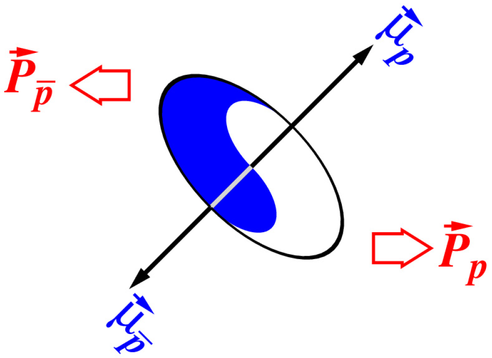
The above-mentioned inverting operations are CPT—transformations (Charge, Parity, and Time reversal symmetry). The CPT theorems prove a strict correspondence between matter and antimatter, between particles and antiparticles. An antiparticle has exactly the same mass and magnetic moment as the particle. However, their electric charges are equal in modulus and opposite in sign. Their spins are also equal in modulus and opposite in direction, Figure 1.

Equations (69) and (70) differ from each other by the signs at the expression $e\hslash c^2(\overrightarrow{\sigma }·\overrightarrow{B})$. The term $e\hslash c^2$ divided by $2m{c}^2$ is named the Bohr magneton ${\mu }_{\mathrm{B}}=e\hslash /2m$. For protons the Bohr magneton is renamed to the nuclear magneton ${\mu }_{\mathrm{N}}$. Its magnetic moment is parallel to the spin while the antiproton has the same magnitude of the magnetic moment but with the opposite sign, Figure 1.

The particle and antiparticle momenta have opposite orientations. From here it follows that these quantum objects revolve about the common mass center. Such a bonded pair is a particle with the integer spin—boson.

Let $|\psi \rangle$ and $|\chi \rangle$ in Equations (69) and (70), accurate to an indeterminate scalar phase, are equal to each other. Now we subtract these equations from each other. We obtain

$$e\hslash c^2(\overrightarrow{\sigma }·\overrightarrow{B})|\psi \rangle =0,$$

(71)

From here it follows that the magnetic field, $\overrightarrow{B}$ as well as the vector potential vanish. It means that the bound pair of the particles expels the existing external magnetic field outside this pair. It is the manifestation of the Meissner effect [53]. Since $\Phi$ and $\overrightarrow{A}$ are zero by adding together Equations (69) and (70) we obtain the Klein-Gordon equation

$${\nabla }^2\Psi -\frac{1}{c^2}\frac{{\partial }^2}{\partial t^2}\Psi =\frac{m^2{c}^2}{{\hslash }^2}\Psi ,$$

(72)

with the wave function $\Psi$ describing relativistic scalar massive fields. There are four Klein-Gordon equations equal to each other. Compare Equations (52) and (72), when the electromagnetic potentials are discarded in the latter.

By repeating computations stated in Section 3 but applied to the Dirac equation with absent $\Phi$ and $\overrightarrow{A}$:

$$\mathbf{i}\hslash {\gamma }^{\mu }{\partial }_{\mu }|\Psi \rangle -mc|\Psi \rangle =0,$$

(73)

we come to a set of four equivalent equations like Equation (72). This equation results from by the following computation—first we multiply the Dirac Equation (73) from the right by $(-\mathbf{i}\hslash {\gamma }_{\mu }{\partial }^{\mu }-mc)$. We obtain:

$$\left({\hslash }^2{\gamma }_{\mu }{\gamma }^{\mu }{\partial }^{\mu }{\partial }_{\mu }+{\left(mc\right)}^2\right)|\Psi \rangle =\left({\hslash }^2\square +m^2{c}^2\right)|\Psi \rangle =0.$$

(74)

It is the Klein-Gordon equation that obeys the “on-shell condition” $p^2={(\hslash ·\overrightarrow{k})}^2=m^2{c}^2$. This equation says: (a) both fermions rotate about the common mass center; (b) the bonded fermions have zero charge; (c) the bonded fermions have integer spin equal to either 0 or ±1; (d) and they have equal masses. It is instructive to note that there are possible spontaneous transitions from bound fermions to the scalar massive waves described by Equation (72) and vice versa.

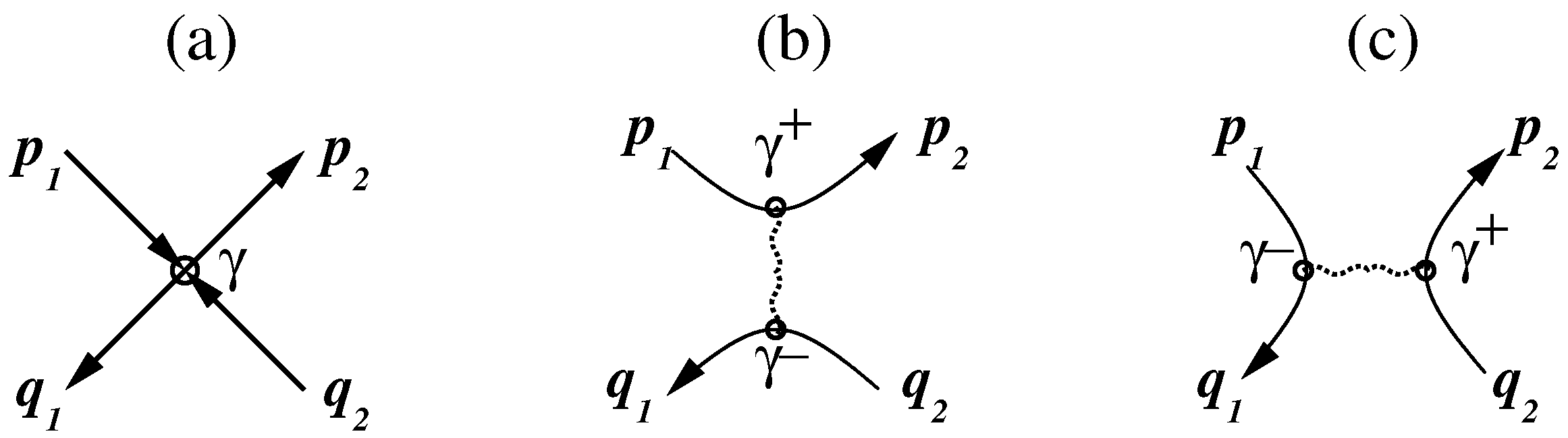
The pair of Dirac fermion fields satisfying the CPT-symmetry [85] points to the existence of the bound particles and antiparticles being bosons. Bosons, unlike fermions, obey Bose-Einstein statistics, which allows an unlimited number of identical particles to be in the same quantum state. The result is the existence of Bose-Einstein condensate. When considering processes leading to Bose-Einstein condensate that go with creation and annihilation of particles and antiparticles, a productive apparatus is the Feynman diagram technique [37]. Figure 2a shows the collision of a particle p and an antiparticle q, which occurs with their instantaneous annihilation and instantaneous birth in the vicinity of the saddle $\gamma$. Such instantaneous reactions are prohibited because they are accompanied by an infinite release of energy. In order to avoid such a singularity, it is assumed that the saddle $\gamma$ splits into two nodes ${\gamma }^{-}$ and ${\gamma }^{+}$, connected to each other by an exchanged quantum with finite energy. There can be two such communication options. The first option assumes elastic scattering Figure 2b, when a particle and an antiparticle are exchanged by an acoustic quantum. The second option is tunneling, when at the node ${\gamma }^{-}$ the particle and antiparticle annihilate with the radiation of a gamma quantum of finite energy Figure 2c, and then this gamma quantum creates a particle–antiparticle pair in the vicinity of the node ${\gamma }^{+}$.

Following the recipes stated in Huang’s book [39] we denote the matrix element for the electron-positron scattering, p-q, by

$$G_{pq}(p_1,q_1;p_2,q_2)=\langle {\overrightarrow{p}}_2,s_2,{\overrightarrow{q}}_2,{\sigma }_2|S^{\left(2\right)}|{\overrightarrow{p}}_1,s_1,{\overrightarrow{q}}_1,{\sigma }_1\rangle$$

(75)

where electron spins are denoted by s and positron spins by $\sigma$. Here bra- and ket- vectors, $\langle f|=\langle {\overrightarrow{p}}_2,s_2,{\overrightarrow{q}}_2,{\sigma }_2|$ and $|i\rangle =|{\overrightarrow{p}}_1,s_1,{\overrightarrow{q}}_1,{\sigma }_1\rangle$, are the final and initial states. $S^{\left(2\right)}$ is the second-order S matrix in the Wick expansion:

$$S^{\left(2\right)}=\frac{1}{2}{(-i{e}_0)}^2\int d^4{x}_1{d}^4{x}_2(I_1+\cdots +I_6).$$

(76)

The operators $I_1,\cdots ,I_6$ contribute to different processes [39], such as (a) disconnecting; (b) e-e scattering; (c) Compton scattering; (d) electron self-energy; (e) photon-self-energy; (f) vacuum process.

Returning to Equation (75), explicitly, the matrix element $G_{pq}(p_1,q_1;p_2,q_2)$ is

$$\begin{array}{ccc}& & G_{pq}(p_1,q_1;p_2,q_2)=\frac{{(-i{e}_0)}^2{m}^2}{\sqrt{E_{p_1}{E}_{q_1}{E}_{p_2}{E}_{q_2}}}\int d^4{x}_1{d}^4{x}_2\hfill \\ & & \times \left[\underset{I}{\underbrace{e^{i(q_1-p_1)x_1-i(q_2-p_2)x_2}\left({\overline{\mathit{v}}}_1{\gamma }^{\mu }{u}_1\right)i{D}_{\mathbf{F}\mu \nu }(x-y){\overline{\mathit{v}}}_2{\gamma }^{\nu }{u}_2)}}-\underset{II}{\underbrace{(q_1\rightleftharpoons q_2)}}\right].\hfill \end{array}$$

(77)

Here $e_0$ is the bare charge, $E_{p_1}=\sqrt{p_1^2+m^2}$, $E_{q_1}=\sqrt{q_1^2+m^2}$, $u_1=u({\overrightarrow{p}}_1,s_1)$, ${\mathit{v}}_1=\mathit{v}({\overrightarrow{q}}_1,{\sigma }_1)$, and so on. The Feynman photon propagator looks as follows

$$D_{\mathbf{F}}^{\mu \nu }(x-y)=-\int \frac{d^{4}k}{{\left(2\pi \right)}^4}\left(g^{\mu \nu }-\lambda \frac{k^{\mu }{k}^{\nu }}{k^2}\right)\frac{e^{-ik·(x-y)}}{k^2+i\eta }$$

(78)

$\eta \to 0_{+}$ and $\lambda$ is the gauge parameter. By choosing $\lambda =0$ we have the so-called Feynman gauge and at $\lambda =1$ Landau gauge.

The first term in Equation (77), I, represents direct electron-positron elastic scattering. The second term, II, represents annihilation.

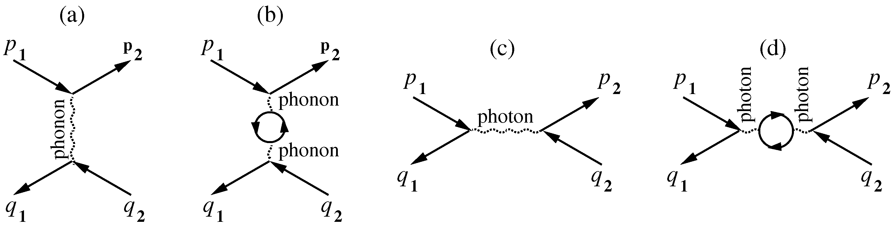
Diagrams in Figure 2b,c give an evident picture of processes going on. Further we will apply the simplest Feynman diagrams showing either the elastic scattering of a particle on an antiparticle, Figure 3a,b, or the tunneling of a particle from one place to another through a barrier when the antiparticle is oncoming tunneling, Figure 3c,d.

Diagrams (a) and (b) depict an elastic scattering of an electron on a positron. Quanta of the elastic scattering are acoustic modes providing so-called the second sound along the space. The second diagram shows a creation with annihilation of a virtual particle by the acoustic quantum. Diagrams (c) and (d) depict tunneling an electron and a positron in themselves at emission and absorption of an electromagnetic (EM) quantum. The second diagram shows a creation with annihilation of a virtual particle by the EM quantum. In both cases, (b) and (d), the virtual particle can be an electron-positron pair, for example.

These simplest diagrams have a high probability of reproduction. Therefore we will take them further as basic building blocks.

4.1. Time Crystal Formation

Returning to Equations (69) and (70), we can remark that there are no direct interactions coupling the wave functions $\varphi$ and $\chi$. There is only a general magnetic field $\overrightarrow{B}$ binding these wave states, accurate to undefined phase multipliers. The latter playing a role of acoustic modes can provide exchanges between these wave states. Such acoustic processes can occur at binding particle-antiparticle pairs at a long-lived configuration, named boson state.

Can the lifetime of an ensemble consisting of many bound particles and antiparticles be large? Let us strike a glance on the examples from the theory of superconductivity. Here, as the Bardeen–Cooper–Schrieffer Theory of Superconductivity says, the main players are electrons bound in Cooper pairs. The superconductivity can happen, so the theory says, when a single negatively charged electron slightly distorts the lattice of atoms in the superconductor, drawing toward it a small excess of positive charges. This excess attracts a second electron. This weak indirect attraction binds the electrons together, into a Cooper pair.

There is a problem with the electrons binding into the Cooper pairs. Boris Vasiliev attracted attention to this problem in 2013 [86,87]. He writes “paired electrons, however, cannot form a superconducting condensate spontaneously. These paired electrons perform disorderly zero-point oscillations and there is no force of attraction in their ensemble. In order to create a unified ensemble of particles, the pairs must order their zero-point fluctuations so that an attraction between the particles appears”.

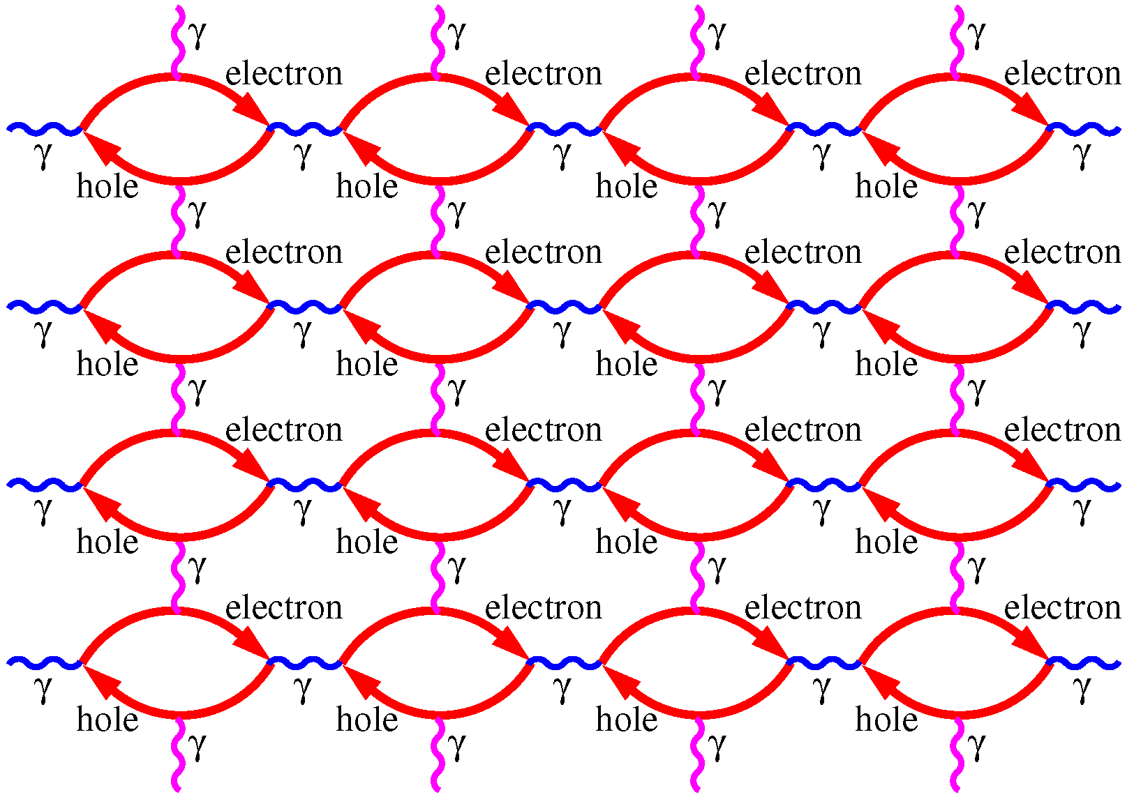
Jorge Hirsch emphasizes a similar thought [88,89], arguing that the traditional theory of superconductivity is incorrect because of the prediction of Joule heating [90] (induced by disordered lattice oscillations). He notes that only bound pairs of electrons and holes can create the Bose particles without dispersion of heat in the normal phase. Such an ensemble of the Bose particles represents by itself the Bose-Einstein long-lived condensate. The whole structure is held together by exchanging gamma quanta, Figure 4. Longitudinal gamma-quanta are quanta of the electromagnetic radiation providing the tunnel effect for electrons and holes forward and backward in time, respectively. While transversal quanta are acoustic modes binding together the electrons and holes as the lattice. These modes provide a so-called second sound.

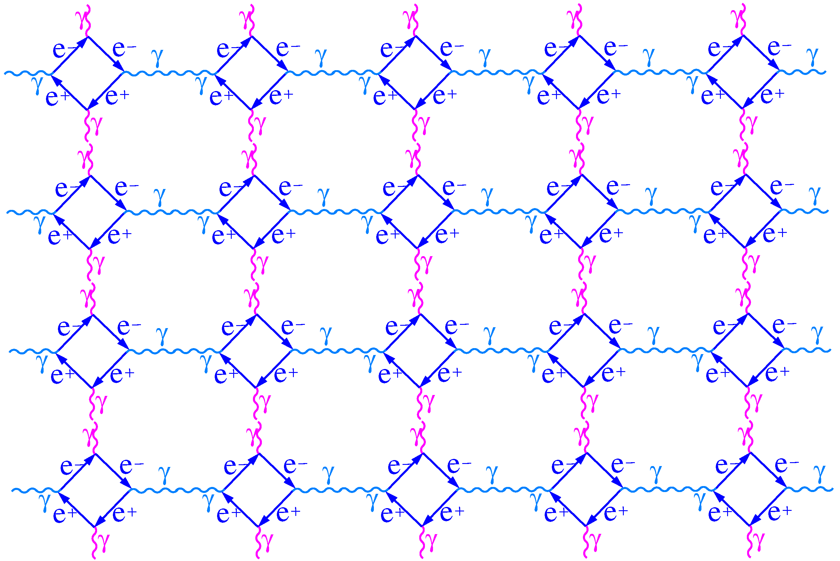
Instead of the holes, antiparticles can be taken. Let us instead of binding electrons with holes shown in Figure 4 take electron-positron pairs, Figure 5. The lifetime of such bonded electron-positron states may be long-lasting enough due to the collective cumulative effect. Similar coherent structures formed from the Bose-Einstein condensates, as shown in Figure 4 and Figure 5, simulate time crystals [56,57,58].

Let the matrix element $G_{pq}(p_1,q_1;p_2,q_2)=\langle {\overrightarrow{p}}_2,s_2,{\overrightarrow{q}}_2,{\sigma }_2|S^{\left(2\right)}|{\overrightarrow{p}}_1,s_1,{\overrightarrow{q}}_1,{\sigma }_1\rangle$ be that of the electron-positron scattering (75), and the functions $|i\rangle =|{\overrightarrow{p}}_1,s_1,{\overrightarrow{q}}_1,{\sigma }_1\rangle$ and $|f\rangle =|{\overrightarrow{p}}_2,s_2,{\overrightarrow{q}}_2,{\sigma }_2\rangle$ are solutions of the Dirac equation. If these solutions have periodical repeating with the period T, then the electron-positron scattering process repeats in time as well.

This periodicity is due to equivalent Feynman diagrams repeating step by step by simulating the stroboscopic effect. The time crystal can manifest itself in ball lightning arising at a thunderstorm. Such macroscopic quantum objects can be capable of tunneling through material obstacles, such as, for example, through window glasses [91,92].

5. Conclusions

Quaternions first discovered by William Rowan Hamilton [1] have had a decisive influence in many areas of scientific knowledge of the world. That is what James Clerk Maxwell, the discoverer of electromagnetic theory, wrote about the discovery of this calculus [93]: “The invention of the calculus of quaternions is a step towards the knowledge of quantities related to space which can only be compared, for its importance, with the invention of triple coordinates by Descartes. The ideas of this calculus, as distinguished from its operations and symbols, are fitted to be of the greatest use in all parts of science”. The quaternion algebra applied to analyzing the 4D space-time manifold discloses promising results covering a wide spectrum of problems.

The set of the quaternions $({\eta }_0,{\eta }_x,{\eta }_y,{\eta }_z)$ gives a possibility to build a set of the differential generating operators due to which shifts in 4D space-time together with rotations and boosts in 3D space are feasible. In this quaternion basis strained over the space-time one can determine the energy-momentum density tensor that contains also all possible forms of rotation motions introduced by organization of the quaternions ${\eta }_x,{\eta }_y,{\eta }_z$.

The transposed set of the quaternions $({\eta }_0,{\eta }_x^{\mathbf{T}},{\eta }_y^{\mathbf{T}},{\eta }_z^{\mathbf{T}})=({\eta }_0,-{\eta }_x,-{\eta }_y,-{\eta }_z)$ added to the original set lead to a possibility to obtain the gravitomagnetic equations that are like the Maxwell equations. Note that the gravitomagnetic equations first were got in a phenomenological way by Oliver Heaviside in 1893 [65] when dealing with the Maxwell equations brought by him to the modern form. That is, he simply noticed between the electromagnetic and gravitational natures many common peculiarities.

It is interesting to note that if we rearrange the order of the computations by the quaternions $({\eta }_0,{\eta }_x^{\mathbf{T}},{\eta }_y^{\mathbf{T}},{\eta }_z^{\mathbf{T}})$ and $({\eta }_0,{\eta }_x,{\eta }_y,{\eta }_z)$, we obtain the same gravitomagnetic equations as if no changes were made, besides the fact that it leads to antimatter. We have considered in the relativistic limit the Dirac fermion fields representing the manifestation of the matter and antimatter fermion fields. These fields on-shell condition, ${(\hslash ·\overrightarrow{k})}^2=p^2=m^2{c}^2$, satisfy the Klein-Gordon equation. This binds the paired particle-antiparticle fermion fields with the electromagnetic field.

From here it follows, in particular, that there can arise self-sustained oscillations between electron-positron bound pairs and quanta of the electromagnetic radiation as shown, for example, in Figure 5. Such oscillations may be provoked at severe thunderstorms or at the moment of powerful stresses of lithospheric plates which are expressed by emergence of the ball lightning, Registration of the positrons at the thunderstorms [94,95] confirms this.

In addition, one can mention yet three sets $({\eta }_0,-{\eta }_x,{\eta }_y,{\eta }_z)$, $({\eta }_0,{\eta }_x,-{\eta }_y,{\eta }_z)$, $({\eta }_0,{\eta }_x,{\eta }_y,-{\eta }_z)$ and their three transposed sets by using of which one can reproduce three addition worlds that are equivalent to the above described. These observations relating to the permutation of signs at the quaternions hints that the same world may pose in different manifestations.

References

- Hamilton, W.R. On quaternions; or a new system of imaginaries in algebra. Phil. Mag. 1844, 25, 489–495. [Google Scholar]
- Agamalyan, M.M.; Drabkin, G.M.; Sbitnev, V.I. Spatial spin resonance of polarized neutrons. A tunable slow neutron filter. Phys. Rep. 1988, 168, 265–303. [Google Scholar] [CrossRef]
- Ioffe, A.I.; Kirsanov, S.G.; Sbitnev, V.I.; Zabiyakin, V.S. Geometric phase in neutron spin resonance. Phys. Lett. A 1991, 158, 433–435. [Google Scholar] [CrossRef]
- Sbitnev, V.I. Passage of polarized neutrons through magnetic media. Depolarization by magnetized inhomogeneities. Z. Phys. B Cond. Matt. 1989, 74, 321–327. [Google Scholar] [CrossRef]
- Sbitnev, V.I. Particle with spin in a magnetic field—The Pauli equation and its splitting into two equations for real functions. Quantum Magic 2008, 5, 2112–2131. (In Russian) [Google Scholar]
- Sbitnev, V.I. Hydrodynamics of superfluid quantum space: Particle of spin-1/2 in a magnetic field. Quantum Stud. Math. Found. 2018, 5, 297–314. [Google Scholar] [CrossRef] [Green Version]
- Sbitnev, V.I. Quaternion Algebra on 4D Superfluid Quantum Space-Time: Gravitomagnetism. Found. Phys. 2019, 49, 107–143. [Google Scholar] [CrossRef] [Green Version]
- Lounesto, P. Clifford Algebras and Spinors; London Mathematical Society Lecture Note. Series 286; Cambridge University Press: Cambridge, UK, 2001. [Google Scholar]
- Girard, P.R. The quaternion group and modern physics. Eur. J. Phys. 1984, 5, 25–32. [Google Scholar] [CrossRef]
- Girard, P.R. Quaternions, Clifford Algebras and Relativistic Physics; Birkhauser Verlag AG: Basel, Switzerland, 2007. [Google Scholar]
- Hong, I.K.; Kim, C.S. Quaternion Electromagnetism and the Relation with Two-Spinor Formalism. Universe 2019, 5, 135. [Google Scholar] [CrossRef] [Green Version]
- Penrose, R. Twistor quantization and curved space-time. Int. J. Theor. Phys. 1968, 1, 61–99. [Google Scholar] [CrossRef]
- Penrose, R. Spinors and torsion in general relativity. Found. Phys. 1983, 13, 325–339. [Google Scholar] [CrossRef]
- Penrose, R.; Rindler, W. Spinors and Space-Time Volume 1: Two-Spinor Calculus and Relativistic Fields; Cambridge University Press: Cambridge, UK, 1984. [Google Scholar]
- Penrose, R.; Rindler, W. Spinors and Space-Time. Volume 2: Spinor and Twistor Methods in Space-Time Geometry; Cambridge University Press: Cambridge, UK, 1986. [Google Scholar]
- Atiyah, M.; Dunajski, M.; Mason, L.J. Twistor theory at fifty: From contour integrals to twistor strings. Proc. R. Soc. A 2017, 473, 20170530. [Google Scholar] [CrossRef]
- Abdullah, M.H.; Klypin, A.; Wilson, G. Cosmological Constraints on Ωm and σ8 from Cluster Abundances Using the GalWCat19 Optical-spectroscopic. Astron. J. 2020, 901, 90. [Google Scholar] [CrossRef]
- Ade, P.A.R. 257 Co-Authors of Planck Collaboration. Planck 2015 results. XIII. Cosmological parameters. Astron. Astrophys. 2016, 594, 1–63. [Google Scholar] [CrossRef] [Green Version]
- Rubin, V.C. A brief history of dark matter. In The Dark Universe: Matter, Energy and Gravity; Livio, M., Ed.; Symposium Series: 15; Cambridge University Press: Cambridge, UK, 2004; pp. 1–13. [Google Scholar]
- Albareti, F.D.; Cembranos, J.A.R.; Maroto, A.L. Vacuum energy as dark matter. Phys. Rev. D 2014, 90, 123509. [Google Scholar] [CrossRef] [Green Version]
- Berezhiani, L.; Khoury, J. Theory of Dark Matter Superfluidity. Phys. Rev. D 2015, 92, 103510. [Google Scholar] [CrossRef] [Green Version]
- Bettoni, D.; Colombo, M.; Liberati, S. Dark matter as a Bose-Einstein Condensate: The relativistic non-minimally coupled case. J. Cosmol. Astropart. Phys. 2014, 2014, 004. [Google Scholar] [CrossRef] [Green Version]
- Chefranov, S.G.; Novikov, E.A. Hydrodynamic vacuum sources of dark matter self-generation in an accelerating universe without a Big Bang. J. Exp. Theor. Phys. 2010, 111, 731–743. [Google Scholar] [CrossRef] [Green Version]
- Chung, D.-Y. Galaxy Evolution by the Incompatibility between Dark Matter and Baryonic Matter. Int. J. Astron. Astrophys. 2014, 4, 374–383. [Google Scholar] [CrossRef] [Green Version]
- Das, S.; Bhaduri, R.K. Dark matter and dark energy from Bose-Einstein condensate. Class. Quant. Grav. 2015, 32, 105003. [Google Scholar] [CrossRef] [Green Version]
- Amendola, L.; Tsujikawa, S. Dark Energy. Theory and Observations; Cambridge University Press: Cambridge, UK, 2010. [Google Scholar]
- Ardey, A. Dark fluid: A complex scalar field to unify dark energy and dark matter. Phys. Rev. D 2006, 74, 043516. [Google Scholar] [CrossRef] [Green Version]
- Huang, K. Dark Energy and Dark Matter in a Superfluid Universe. Int. J. Mod. Phys. A 2013, 28, 1330049. [Google Scholar] [CrossRef]
- Nouri-Zonoz, M.; Koohbor, J.; Ramezani-Aval, H. Dark fluid or cosmological constant: Why there are different de Sitter-type spacetimes. Phys. Rev. D 2015, 91, 063010. [Google Scholar] [CrossRef] [Green Version]
- Nouri-Zonoz, M.; Nourizonoz, A. Static and stationary dark fluid universes: A gravitoelectromagnetic perspective. Sci. Rep. 2022, 12, 15032. [Google Scholar] [CrossRef]
- Sbitnev, V.I. Quaternion Algebra on 4D Superfluid Quantum Space-Time: Can Dark Matter Be a Manifestation of the Superfluid Ether? Universe 2021, 7, 32. [Google Scholar] [CrossRef]
- Sbitnev, V.I. Quaternion Algebra on 4D Superfluid Quantum Space-Time. Dirac’s Ghost Fermion Fields. Found. Phys. 2022, 52, 19. [Google Scholar] [CrossRef]
- Volovik, G.E. The Universe in a Helium Droplet; Oxford University Press: Oxford, UK, 2003. [Google Scholar]
- Volovik, G.E. Vacuum energy: Quantum hydrodynamics vs. quantum gravity. JETP Lett. 2005, 82, 319–324. [Google Scholar] [CrossRef] [Green Version]
- Volovik, G.E. The superfluid universe. In Novel Superfluids; Bennemann, K.H., Ketterson, J.B., Eds.; Oxford University Press: Oxford, UK, 2013; Volume 1, Chapter 11; pp. 570–618. [Google Scholar]
- Huang, K. A Superfluid Universe; World Scientific Publ. Co. Pte. Ltd.: Singapore, 2017. [Google Scholar]
- Feynman, R.P.; Hibbs, A. Quantum Mechanics and Path Integrals; McGraw Hill: New York, USA, 1965. [Google Scholar]
- Makri, N. Feynman path integration in quantum dynamics. Comput. Phys. Commun. 1991, 63, 389–414. [Google Scholar] [CrossRef]
- Huang, K. Quantum Field Theory: From Operators to Path Integrals; WILEY-VCH Verlag GmbH & Co. KGaA: Wemheim, Germany, 2004. [Google Scholar]
- Jishi, R.A. Feynman Diagram Techniques in Condensed Matter Physics; Cambridge University Press: Cambridge, UK, 2013. [Google Scholar]
- Prunotto, A.; Alberico, W.M.; Czerski, P. Feynman diagrams and rooted maps. Open Phys. 2018, 16, 149–167. [Google Scholar] [CrossRef] [Green Version]
- Cartan, E. Sur une définition géométrique du tenseur d’énergie d’Einstein. C. R. Acad. Sci. 1922, 174, 437. [Google Scholar]
- Cartan, E. Sur une généralisation de la notion de courbure de Ricmann et les espaces á torsion. C. R. Acad. Sci. 1922, 174, 593–595. [Google Scholar]
- Trautman, A. Einstein-Cartan Theory. arXiv 2006. [Google Scholar] [CrossRef]
- Blixt, D.; Ferraro, R.; Golovnev, A.; Guzmán, M.J. Lorentz gauge-invariant variables in torsion-based theories of gravity. Phys. Rev. D 2022, 105, 084029. [Google Scholar] [CrossRef]
- Einstein, A. Sidelights on Relativity. I. Ether and Relativity, II. Geometry and Experience; Methuen & Co. Ltd.: London, UK, 1922. [Google Scholar]
- Sinha, K.P.; Sudarshan, E.C.G. The superfluid as a source of all interactions. Found. Phys. 1978, 8, 823–831. [Google Scholar] [CrossRef]
- Sinha, K.P.; Sivaram, C.; Sudarshan, E.C.G. Aether as a Superfluid State of Particle-Antiparticle Pairs. Found. Phys. 1976, 6, 65–70. [Google Scholar] [CrossRef]
- Sinha, K.P.; Sivaram, C.; Sudarshan, E.C.G. The superfluid vacuum state, time-varying cosmological constant, and nonsingular cosmological models. Found. Phys. 1976, 6, 717–726. [Google Scholar] [CrossRef]
- Boehmer, C.G.; Harko, T. Can dark matter be a Bose-Einstein condensate? J. Cosmol. Astropart. Phys. 2007, 2007, 25. [Google Scholar] [CrossRef] [Green Version]
- Harko, T.; Mocanu, G. Cosmological evolution of finite temperature Bose-Einstein Condensate dark matter. Phys. Rev. D 2012, 85, 084012. [Google Scholar] [CrossRef] [Green Version]
- Crâciun, M.; Harko, T. Testing Bose-Einstein Condensate dark matter models with the SPARC galactic rotation curves data. Eur. Phys. J. 2020, 20. [Google Scholar] [CrossRef]
- Meissner, W.; Ochsenfeld, R. Ein neuer Effekt bei Eintritt der Supraleitfähigkeit. Naturwissenschaften 1933, 21, 787–788. [Google Scholar] [CrossRef]
- Else, D.V.; Bauer, B.; Nayak, C. Floquet Time Crystals. Phys. Rev. Lett. 2016, 117, 090402. [Google Scholar] [CrossRef] [PubMed] [Green Version]
- Lounasmaa, O.V.; Thuneberg, E. Vortices in rotating superfluid 3He. Proc. Natl. Acad. Sci. USA 1999, 96, 7760–7767. [Google Scholar] [CrossRef] [PubMed] [Green Version]
- Sacha, K.; Zakrzewski, J. Time crystals: A review. Rep. Prog. Phys. 2018, 81, 016401. [Google Scholar] [CrossRef] [PubMed]
- Muõz Arias, M.H.; Chinni, K.; Poggi, P.M. Floquet time crystals in driven spin systems with all-to-all p-body interactions. Phys. Rev. Res. 2022, 4, 023018. [Google Scholar] [CrossRef]
- Wilczek, F. Quantum Time Crystals. Phys. Rev. Lett. 2012, 109, 160401. [Google Scholar] [CrossRef] [Green Version]
- Dirac, P.A.M. Is there an Aether? Nature 1951, 168, 906–907. [Google Scholar] [CrossRef]
- Petroni, N.C.; Vigier, J.P. Dirac’s Aether in Relativistic Quantum Mechanics. Found. Phys. 1983, 13, 253–286. [Google Scholar] [CrossRef]
- Sbitnev, V.I. Quaternion algebra on 4D superfluid quantum space-time (in: 4rd International Conference on High Energy Physics, 3–4 December 2018, Valencia, Spain). J. Astrophys. Aerosp. Technol. 2018, 6, 55–56. [Google Scholar]
- Sbitnev, V.I. Quaternion Algebra on 4D Superfluid Quantum Space-Time: Equations of the Gravitational-Torsion Fields. In Proceedings of the SCON International Convention on Astro Physics and Particle Physics, Amsterdam, The Netherlands, 23–24 May 2019. [Google Scholar]
- Jackiw, R.; Nair, V.P.; Pi, S.Y.; Polychronakos, A.P. Perfect Fluid Theory and its Extensions. J. Phys. A 2004, 37, R327–R432. [Google Scholar] [CrossRef] [Green Version]
- Nelson, E. Derivation of the Schrödinger equation from Newtonian Mechanics. Phys. Rev. 1966, 150, 1079–1085. [Google Scholar] [CrossRef]
- Heaviside, O. A gravitational and electromagnetic analogy. Electrician 1893, 31, 281–282. [Google Scholar]
- Jantzen, R.T. The Many Faces of Gravitoelectromagnetism. Ann. Phys. 1992, 215, 1–50. [Google Scholar] [CrossRef] [Green Version]
- Mashhoon, B.; Gronwald, F.; Lichtenegger, H.I.M. Gravitomagnetism and the Clock Effect. Lect. Notes Phys. 2001, 562, 83–108. [Google Scholar]
- Kopeikin, S.; Mashhoon, B. Gravitomagnetic effects in the propagation of electromagnetic waves in variable gravitational fields of arbitrary-moving and spinning bodies. Phys. Rev. D 2002, 65, 064025. [Google Scholar] [CrossRef] [Green Version]
- Behera, H.; Naik, P.C. Gravitomagnetic Moments and Dynamics of Dirac (spin 1/2) fermions in flat space-time Maxwellian Gravity. Int. J. Mod. Phys. A 2004, 19, 4207–4230. [Google Scholar] [CrossRef] [Green Version]
- Khmelnik, S.I. Gravitomagnetism: Nature’s Phenomenas, Experiments, Mathematical Models; Mathematics in Computer Corp: Bene-Ayish, Israel, 2017. [Google Scholar] [CrossRef]
- Bocker, R.P.; Frieden, B.R. A new matrix formulation of the Maxwell and Dirac equations. Heliyon 2018, 4, e01033. [Google Scholar] [CrossRef]
- Landau, L.; Lifshitz, E. The Classical Theory of Fields; Elsevier: Amsterdam, The Netherlands, 2005. [Google Scholar]
- Güveniş, H. Hydrodynamic Formulation of Quantum Electrodynamics. Gen. Sci. J. 2014, 9, 1–8. [Google Scholar]
- Majorana, E. A symmetric theory of electrons and positrons. Il Nuovo C. 1937, 14, 171–184. [Google Scholar] [CrossRef]
- Kernbach, S. Electrochemical characterisation of ionic dynamics resulting from spin conversion of water isomers. J. Electrochem. Soc. 2022, 169, 067504. [Google Scholar] [CrossRef]
- Madelung, E. Quantumtheorie in hydrodynamische form. Zts. F. Phys. 1926, 40, 322–326. [Google Scholar] [CrossRef]
- de Broglie, L. Interpretation of quantum mechanics by the double solution theory. Ann. Fond. Louis Broglie 1987, 12, 1–22. [Google Scholar]
- Bohm, D. A Suggested Interpretation of the Quantum Theory in Terms of “Hidden” Variables. I. Phys. Rev. 1952, 85, 166–179. [Google Scholar] [CrossRef]
- Bohm, D. A Suggested Interpretation of the Quantun Theory in Terms of “Hidden” Variables. II. Phys. Rev. 1952, 85, 180–193. [Google Scholar] [CrossRef]
- Ginzburg, V.L.; Landau, L.D. On the theory of superconductivity. Z. Eksp. Teor. Fiz 1950, 20, 1064. [Google Scholar]
- Nelson, E. Dynamical Theories of Brownian Motion; Princeton University Press: Princeton, NJ, USA, 1967. [Google Scholar]
- Nelson, E. Review of stochastic mechanics. J. Phys. Conf. Ser. 2012, 361, 012011. [Google Scholar] [CrossRef]
- Nelson, E. Quantum Fluctuations; Princeton Series in Physics; Princeton University Press: Princeton, NJ, USA, 1985. [Google Scholar]
- Sbitnev, V.I. Generalized path integral technique: Nanoparticles incident on a slit grating, matter wave interference. In Advances in Quantum Mechanics; Bracken, P., Ed.; InTech: Rijeka, Croatia, 2013; Chapter 9; pp. 183–211. [Google Scholar] [CrossRef] [Green Version]
- Tureanu, A. CPT and Lorentz Invariance: Their Relation and Violation. J. Phys. Conf. Ser. 2013, 474, 012031. [Google Scholar] [CrossRef] [Green Version]
- Vasiliev, B.V. Superconductivity and Superfluidity. Univers. J. Phys. Appl. 2013, 1, 392–407. [Google Scholar] [CrossRef]
- Vasiliev, B.V. Superconductivity and Superfluidity; Science Publishing Group: New York, NY, USA, 2015. [Google Scholar]
- Hirsch, J.E. Superconductivity, what the H? The emperor has no clothes. arXiv 2020. [Google Scholar] [CrossRef]
- Hirsch, J.E. Thermodynamic inconsistency of the conventional theory of superconductiv. Int. J. Mod. Phys. B 2020, 34, 2050175. [Google Scholar] [CrossRef]
- Nikulov, A. The Law of Entropy Increase and the Meissner Effect. Entropy 2022, 24, 83. [Google Scholar] [CrossRef]
- Bychkov, V.L.; Nikitin, A.I.; Ivanenko, I.P.; Nikitina, T.F.; Velichko, A.M.; Nosikov, I.A. Ball lightning passage through a glass without breaking it. J. Atmos. Sol.-Terr. Phys. 2016, 150–151, 69–76. [Google Scholar] [CrossRef]
- Grigoriev, A. Attention—Ball lightning. Tekhnika Molod. 1982, 2, 49–50. (In Russian) [Google Scholar]
- Maxwell, J.C. Remarks on the mathematical classification of physical quantities. Proc. Lond. Math. Soc. 1869, 3, 224–232. [Google Scholar] [CrossRef]
- Enoto, T.; Wada, Y.; Furuta, Y.; Nakazawa, K.; Yuasa, T.; Okuda, K.; Makishima, K.; Sato, M.; Sato, Y.; Tsuchiya, H.; et al. Photonuclear reactions triggered by lightning discharge. Nature 2017, 552, 481–484. [Google Scholar] [CrossRef] [Green Version]
- Wu, H.C. Relativistic-microwave theory of ball lightning. Sci. Rep. 2016, 6, 28263. [Google Scholar] [CrossRef]
Figure 1.
Proton–antiproton pair has opposite oriented magnetic moments, and , and opposite directed momenta and . They revolve about the mass center.
Figure 2.
The diagrams show conditionally the scattering of the particle p on antiparticle q: (a) this diagram is defective, since there is an infinite release of energy in the vicinity of the collision point . The real diagrams accompanied by the exchange of gamma quanta with finite energy are diagrams of (b) elastic scattering of a particle and an antiparticle (exchange) and (c) tunneling through a finite barrier (annihilation and creation). The wavy dotted line represents an incoming or outgoing photon . Solid lines with arrows point along the direction of flow of electron charge (it is either an electron, p, propagating from the left to right, or a positron, q, propagating in the opposite direction).
Figure 3.
Particles (in this case, electron p) move from left to right (forwards in the future), antiparticles (in this positron q) move from right to left (back in the past). Elastic scattering, shown in (a,b), happens due to exchanging acoustic quanta being perturbed within the quantum normal phase. Tunneling, shown in (c,d), represents the annihilation of particles and antiparticles with the radiation of an electromagnetic (EM) quantum in one space area and creation of them in the remote space area with the absorption of the EM quantum. Subfigures (b,d) demonstrate the creation with annihilation of a virtual particle-antiparticle loop.
Figure 4.
An ordered ensemble of electron-hole pairs simulating the time crystal [56,57,58]. Vertical wavy curves depict phonon (the second sound) excitations coupling the pairs in the self-sustained ensemble. Horizontal wavy curves represent EM photons providing a coherent continuation (tunneling) of electron-hole quantized pairs in time.
Figure 5.
Self-sustained macroscopic Bose-Einstein condensate consisting of the electrons and positrons. This lattice is a perfect simulation of the time crystal.
Disclaimer/Publisher’s Note: The statements, opinions and data contained in all publications are solely those of the individual author(s) and contributor(s) and not of MDPI and/or the editor(s). MDPI and/or the editor(s) disclaim responsibility for any injury to people or property resulting from any ideas, methods, instructions or products referred to in the content. |
© 2023 by the author. Licensee MDPI, Basel, Switzerland. This article is an open access article distributed under the terms and conditions of the Creative Commons Attribution (CC BY) license (https://creativecommons.org/licenses/by/4.0/).
Share and Cite
MDPI and ACS Style
Sbitnev, V. Relativistic Fermion and Boson Fields: Bose-Einstein Condensate as a Time Crystal. Symmetry 2023, 15, 275. https://doi.org/10.3390/sym15020275
AMA Style
Sbitnev V. Relativistic Fermion and Boson Fields: Bose-Einstein Condensate as a Time Crystal. Symmetry. 2023; 15(2):275. https://doi.org/10.3390/sym15020275
Chicago/Turabian StyleSbitnev, Valeriy. 2023. "Relativistic Fermion and Boson Fields: Bose-Einstein Condensate as a Time Crystal" Symmetry 15, no. 2: 275. https://doi.org/10.3390/sym15020275
Note that from the first issue of 2016, this journal uses article numbers instead of page numbers. See further details here.