
Timelike Circular Surfaces and Singularities in Minkowski 3-Space


1
School of Mathematics, Hangzhou Normal University, Hangzhou 311120, China
2
Mathematical Science Department, Faculty of Science, Princess Nourah bint Abdulrahman University, Riyadh 11546, Saudi Arabia
3
Department of Mathematics, Faculty of Science, University of Assiut, Assiut 71516, Egypt
*
Author to whom correspondence should be addressed.
Symmetry 2022, 14(9), 1914; https://doi.org/10.3390/sym14091914
Submission received: 26 July 2022
/
Revised: 28 August 2022
/
Accepted: 6 September 2022
/
Published: 13 September 2022
(This article belongs to the Section Mathematics)
Abstract
:The present paper is focused on time-like circular surfaces and singularities in Minkowski 3-space. The timelike circular surface with a constant radius could be swept out by moving a Lorentzian circle with its center while following a non-lightlike curve called the spine curve. In the present study, we have parameterized timelike circular surfaces and examined their geometric properties, such as singularities and striction curves, corresponding with those of ruled surfaces. After that, a different kind of timelike circular surface was determined and named the timelike roller coaster surface. Meanwhile, we support the results of this work with some examples.
1. Introduction
In spatial kinematics, the movement of the one-parameter family of circles with stationary radius constructs a circular surface, while the movement of the one-parameter family of lines constructs a ruled surface. A circular surface has a spine curve, and a ruled surface has a striction curve. The envelope of the tangent lines to a space curve defines a tangent developable ruled surface. The characteristics of a tangent ruled surface are straight lines which are tangential to the edge of regression. The edge of regression designates singular points of the tangent developable ruled surface [1,2,3,4,5,6]. With an analogous notion for ruled surfaces, geometers have investigated circular surfaces in the Euclidean and Minkowski 3-spaces. For example, Izumiya et al. [7] discussed several geometric possessions and singularities of circular surfaces corresponding with ruled surfaces. In [8], the authors initiated great circular surfaces which were generated as a one-parameter family of great circles in three spheres, and they gained a comprehensive classification of the singularities of such surfaces while also discussing the geometric explanations via points of spherical geometry. In [9], a new denomination of circular surfaces in Euclidean 3-space was considered by a curve and a conformity of circles. The authors particularly inspected some geometrical characterizations of circular surfaces in case the base curve was an algebraic curve. Spacelike circular surfaces in Minkowski 3-space are introduced, and several geometric possessions are obtained [10]. Furthermore, the authors defined spacelike roller coaster surfaces as spacelike circular surfaces in the case when the generated circles were curvature lines. Tuncer et al. [11] defined the equations of a spacelike circular surface and spacelike roller coaster surface depending on the unit split quaternions and homothetic movements. In [12], Nadia Alluhaibi presented some new results regarding circular surfaces in Euclidean 3-space. Nadia Alluhaibi also showed the conditions for the roller coaster surfaces to be minimal surfaces or flat. In [13], R. Abdel-Baky et al. studied timelike circular surfaces in Minkowski 3-space. However, they did not consider the singularities’ properties. In this work, we consider the geometrical possessions and singularity of a timelike circular surface with a stationary radius in Minkowski 3-space . In Section 3, we address a timelike circular surface and obtain its Gaussian and mean curvature. Then, we examine the conditions of the curve in order to form striction curves on the timelike circular surface. Then, we present a characterization of local singular points on timelike circular surfaces. In the case of every generated circle with a curvature line, except for the singular or umbilical points, a classification of such timelike circular surfaces into Lorentzian spheres, timelike canal surfaces, a special type of timelike surfaces or timelike surfaces is regularly linked the three surfaces. At the end, certain examples are given to support the idea of how to form the timelike roller coaster and timelike circular surface.
2. Basic Concepts
For this study, we begin with certain concepts that will be used later [14,15,16]. Suppose , (i = 1, 2, 3)} is a 3-dimensional Cartesian space. For all and , the Lorentzian scalar product of and is given as follows:
defines the Minkowski 3-space, and we use it as an alternative to (. A non-zero vector defines whether it is spacelike, lightlike or timelike in the case where , or in the same order. The norm of is . Furthermore, for two vectors and the cross product is
where , , is the canonical basis of . The hyperbolic and Lorentzian unit spheres, are the following:
and
Definition 1.
- (i)
- Spacelike angle: If as well as are spacelike vectors at which span a spacelike vector subspace, then , and a unique real number exists that is . It is named the spacelike angle between and .
- (ii)
- Central angle: If and are spacelike vectors at which span a timelike vector subspace, then , and a unique real number exists that is . It is named the central angle between and .
- (iii)
- Lorentzian timelike angle: If is a spacelike vector and is a timelike vector at , then a unique real number exists that is . This is the Lorentzian timelike angle among and .
We indicate the surface M at as follows:
Suppose is a standard unit normal vector field on a surface M determined using , where . Therefore, the first fundamental form (metric) I of the surface M is given as
where , . In addition, the second fundamental form of M will be as follows:
where , . The Gaussian curvature K and the mean curvature H are
where . A surface in the Minkowski 3-space names a spacelike or timelike surface in case the induced metric at the surface is a positive or negative definite Riemannian metric, respectively. This is identical to stating that the normal vector on the spacelike or timelike surface is a timelike or spacelike vector, respectively [1,2,3].
3. Timelike Circular Surfaces
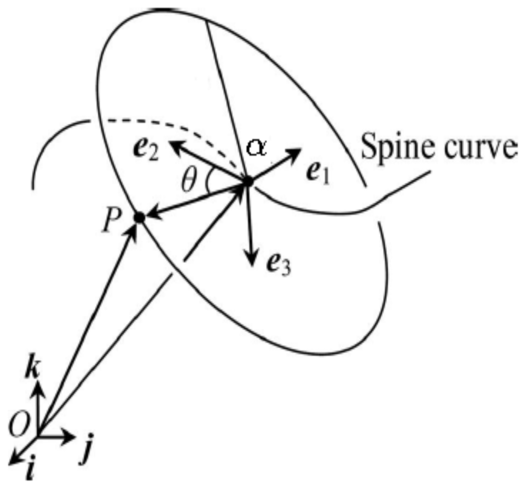
We consider the notion of timelike circular surfaces in . Let us have a non-null curve as a regular curve with its tangent vectors such that for all , and a positive number , a timelike circular surface is defined as the surface which is swept out using a set of timelike circles with its center points following the curve . Either circle names a generating circle, which lies on a Lorentzian plane named the circle plane. Assuming indicates the timelike unit normal vector of a circle plane, and is connected to all points of the spine curve , when given a radius r of a generating circle, a timelike circular surface is specified using and . Henceforth, this work represents the derivative with respect to u with primes.
In this case, u is the arc length of the spacelike spherical curve , and the unit spacelike tangent vector of is . We also have a spacelike unit vector , and then we define an orthonormal moving frame along . This is named the Blaschke frame of the spherical curve . It is clear that
Therefore, we have the following Blaschke formulae:
where is the spherical or geodesic curvature of . Let us express the tangent vector as
where , and define its coordinate functions. Suppose and construct the basis of the corresponding circle plane at all points of the spine curve . Therefore, for a sufficient small parameter , and using the solutions of the differential system in Equation (6), the timelike circular surface M is constructed as follows:
We call a spine curve, and is named a generating circle (Figure 1) [6]. , and define a complete system of curvature functions (invariants) of the surface M.
In this paper, we do not consider timelike circular surfaces with fixed vectors . Clearly, Equation (8) gives a method for constructing timelike circular surfaces with a radius by the following equation:
The tangent vectors are
Then, we have
The spacelike unit normal vector for M is presented as
By a straightforward calculation, we find
Then, we have
The following definition is helpful:
Definition 2.
Assume M is the timelike circular surface with Equation (8). Therefore, at , the following holds:
- (1)
- M is named a timelike canal (tubular) surface in the case where the spine curve is perpendicular to the circular plane such that , and satisfy
- (2)
- M is named a timelike roller coaster (or tangent) surface in the case where the spine curve is a tangent to the circular plane such that , and satisfy
A thorough treatment on timelike roller coaster surfaces will be given latter.
3.1. Striction Curves
As we know, the lines are the simplest examples of curves, and circles with a stationary radius give other simple examples of curves. Ruled surfaces are formed by a family of lines, and circular surfaces are formed by a set of circles with a stationary radius. Ruled surfaces have striction curves, and circular surfaces have spine curves. As a result, it is normal to investigate circular surfaces as an analogy with the ruled surfaces. Thus, for the timelike circular surface M, the curve
is the striction curve if ensures
This is equivalent to
From Equation (18), it follows that striction points only exist when
Hence, two striction curves exist and are represented by
In light of Equations (15) and (20), all curves on the timelike canal surface transverse to the generating circles ensure the condition of the striction curves; that is, . As a result, the sets of timelike canal surfaces are an analogous class to the sets of Lorentzian cylindrical surfaces:
Proposition 1.
Any non-canal timelike circular surface has two striction curves and intersects with every generating circle. Lorentzian circles are antipodal points to each other.
3.2. Curvature Lines and Singularities
Here, we consider timelike circular surfaces whose generating circles are curvature lines, except for umbilical points or singular points. Using Equations (10) and (12), it is clear that all generating circles are curvature lines if
We will now research this situation in detail. In case , then M cannot be generated. (In reality, we have assumed .) In addition, if , then the surface M is not regular. As stated in the assumption of M being regular, we find
for all . Then, we have the following:
- Case (1)
- When , then ; that is, the spine curve is a fixed point. This means that the timelike circular surface is a Lorentzian sphere with a radius r. Namely, .
- Case (2)
- When , the spine curve is orthogonal to the spacelike circular plane; that is, is parallel to . Therefore, the timelike circular surface turns into a timelike canal surface with a timelike spine curve.
- Case (3)
- When , the tangent vector is parallel to . Hence, the tangent vector of the spine curve lies at the spacelike circle plane for all points of M. Specifically, . When is constant, consequently, we havewhere is a constant vector. However, using Eqations (8) and (23) leads toThis implies that all the circle points lie on a Lorentzian sphere of a radius , with being its center point in .
After the above explanation we give the following theorem:
Theorem 1.
In the Minkowski 3-space , aside from the general timelike circular surfaces, there are two sets of timelike circular surfaces whose generating circles are curvature lines. These two sets are the timelike roller coaster surfaces and the Lorentzian spheres with a radius less than that of the generating circles.
Singularities are essential for aspects of timelike circular surfaces and are defined as follows. In Equations (6)–(9), it is shown that M has a singular point at if
This yields two (linearly dependent) equations:
The singular points are discussed as follows:
- Case (1)
- This exists when . If and , then the singular points are located at and . If and , then the singular points are located at . If , for a timelike circular surface to have singular points, it is necessary that . Therefore, there are two singular points on the generating circle, located at .
- Case (2)
- This exists if . In the case of a timelike circular surface having singular points, it is necessary that . Since , we can say that the singularities are only located when and . Thus, there are two singular points on each generating circle. Adding these two sets of singular points results in two curves (striction curves) that contain all the singular points of a timelike circular surface. Then, the striction curves form a timelike circular surface.
Under the above notations, it might be said that the geometrical properties of timelike circular surfaces are analogues with those of developable ruled surfaces. Lorentzian spheres correspond to cones, timelike canal surfaces to cylinders and timelike roller coaster surfaces to tangent developable surfaces. Hence, the following corollary can be given:
Corollary 1.
Suppose M is a timelike circular surface which has generating circles as curvature lines, except at umbilical points or singular points. Therefore, M is a part of a Lorentzian sphere, a timelike canal surface and a timelike roller coaster surface.
3.3. Timelike Canal (Tubular) Surfaces
Here, we check and construct a timelike canal surface () whose parametric curves are curvature lines. Then, using Eqations (11) and (14), we consequently have . If we use this in Equation (6), we obtain the following ODE:
From this equation, the spherical curve can be represented as
which is a timelike unit vector. Clearly, we have
Assuming an integral with zero integration constants yields
Let us choose . Therefore, we have
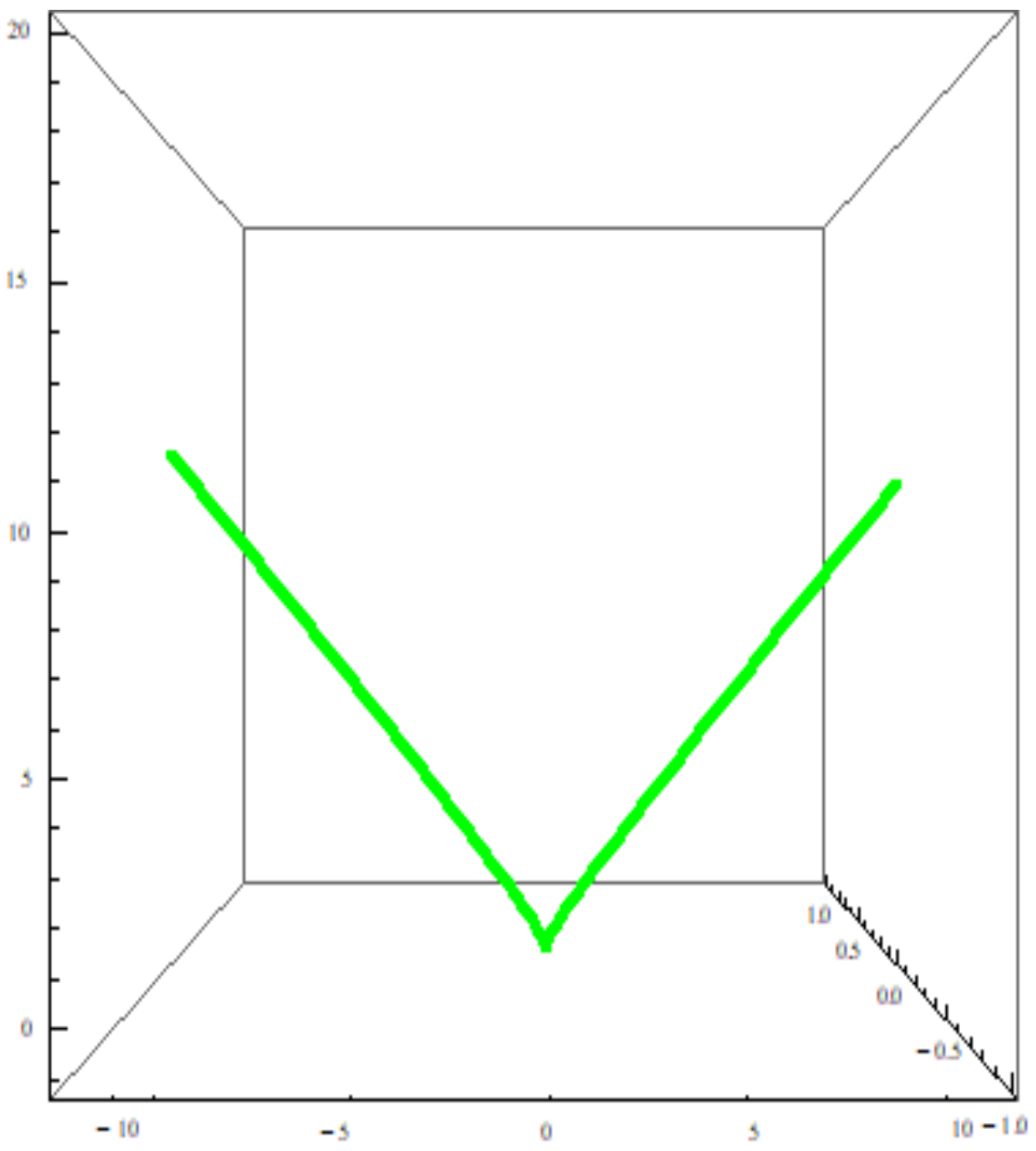
It is clear that has a singular point (cusp) at (Figure 2). Thus, the timelike canal surface M with the timelike spine curve is given by
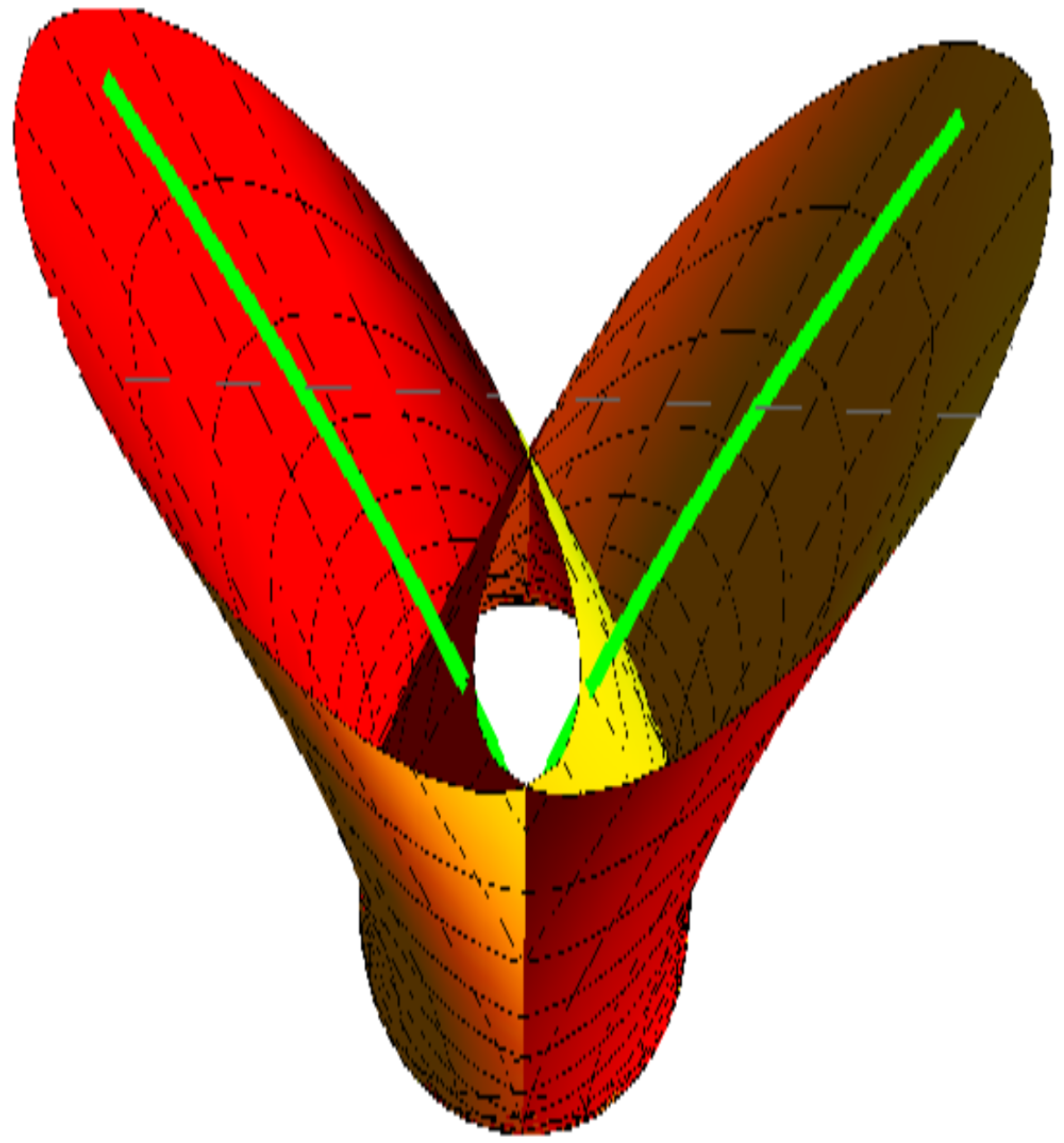
For , with and , the surface is illustrated in Figure 3.
We now give an example regarding singularity and the striction curve of a non-canal timelike circular surface:
Example 1.
A non-canal timelike circular surface can be defined as follows. Take the Blaschke frame as shown in Equation (27) and . Then, it is easy to derive
which shows that has no singular point. Then, according to Equation (20), the striction curves are
The timelike circular surface M with the spine curve is then given by
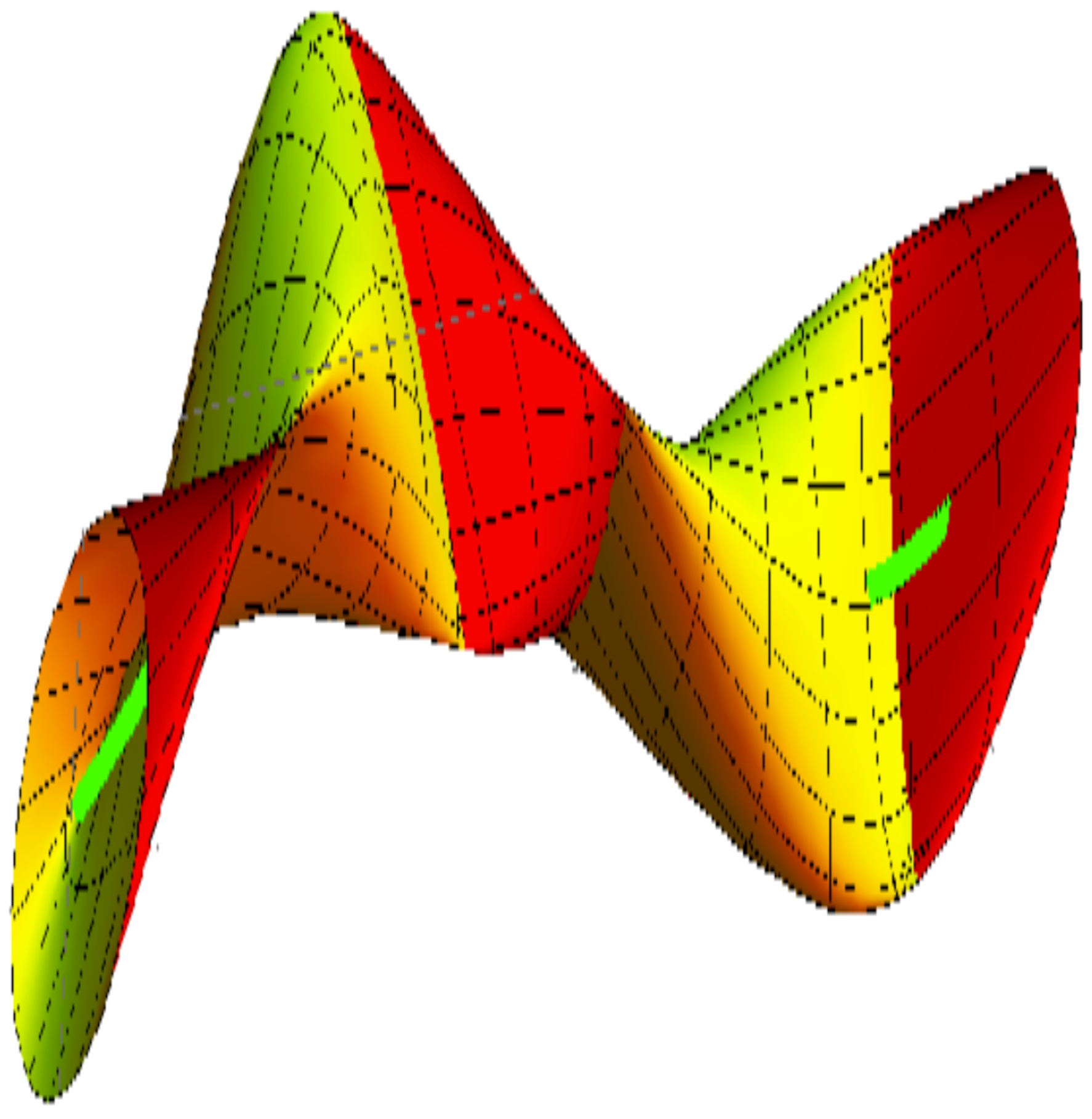
which has different singularities appear on the striction curves (green), where , with and (Figure 4).
3.4. Timelike Canal (Tubular) Surface
We now derive a parametric representation of a timelike canal (tubular) surface with a timelike spine curve. Consider s to be the arc length parameter of and , to be its Serret–Frenet frame. Then, we have
and
where and define the natural curvature and torsion:
Notably, as long as is perpendicular to the circle planes at all points of the spine curve, the canal surface can be defined as
The tangent vectors are
where such that
and
Then, we have
Therefore, we can write
Hence, the Gaussian and mean curvatures can be calculated as
On the other hand, because every Lorentzian generating circle is a curvature line, the value of one principal curvature is
The principle direction of points in the direction of the Lorentzian generating circle, and this curvature is constant:
Corollary 2.
The principal curvature of a timelike canal surface is constant along all generating Lorentzian circles.
Example 2.
Let be a unit speed timelike helix. Clearly, we have
Hence, we construct the timelike canal surface as follows:
The spine curve has no singular points. Clearly, has different singularities with and (Figure 5).
3.5. Timelike Roller Coaster Surfaces
Timelike roller coaster surfaces are considered to be those where the tangent vector of the spine curve lies in the spacelike circle plane at all points of . This means that , and do not equal zero simultaneously. Through this work, we will only assume that and . If so, such a surface is called a timelike roller coaster surface with a spacelike spine curve; that is, . From Equation (19), it follows that and . Hence, the equation of the striction curves is
which contains all the singular points. Therefore, striction curves form a timelike roller coaster surface with a spacelike spine curve. The curvature and torsion may be derived, depending on and , as follows:
Thus, if is a constant, then the torsions are zero simultaneously; that is, the striction curves are planar spacelike curves. Moreover, the Gaussian and mean curvatures at a regular point can be written as
It is a noteworthy fact that concepts such as both Gaussian curvature and principal curvatures, whose definition makes fundamental use of the location of a surface in a space, do not rely on the geodesic curvature of but only on and . Hence, the following conclusions can be given:
Theorem 2.
If a set of timelike roller coaster surfaces has an equal radius and scalar σ, and its derivative is , then the Gaussian as well as the mean curvatures at corresponding points will be equal to each other at the corresponding point. Moreover, their values are independent of the geodesic curvature of the hyperbolic spherical image curve .
Furthermore, to study the kinematic-geometric possessions of the timelike roller coaster surface, the Serret–Frenet of the spine curve is necessary to build. Therefore, assume v be the arc length of the spacelike spine curve and at all , where the Serret–Frenet frame of the spine curve can be presented as
By letting , it follows that
Thus, we have
where
The timelike roller coaster surface can be presented as
Furthermore, the two striction curves are
As in the previous equations, we not only prove the existence of the timelike roller coaster, but we also give the specified expression of the surface. This is very significant in practical application.
A surface with zero Gaussian curvature is called a flat surface. Clearly, M is flat if . Thus, for every , we have
Using Equations (32) and (34), the indication of in terms of the Serret–Frenet invariants is
Therefore, in a neighborhood of every point on M with , we have . Therefore, a timelike roller coaster surface whose Gaussian curvature vanishes identically is a part of the timelike plane. In the same method, we find that M is a timelike minimal flat surface. Hence, we state the following:
Corollary 3.
All the flat (minimal) timelike roller coaster surfaces are subsets of Lorentzian planes.
Example 3.
Take the case of a parametric spacelike circular helix, such as
With normal computation, we have
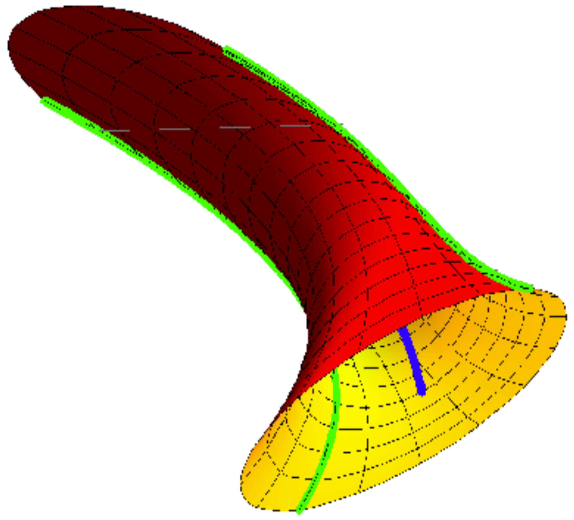
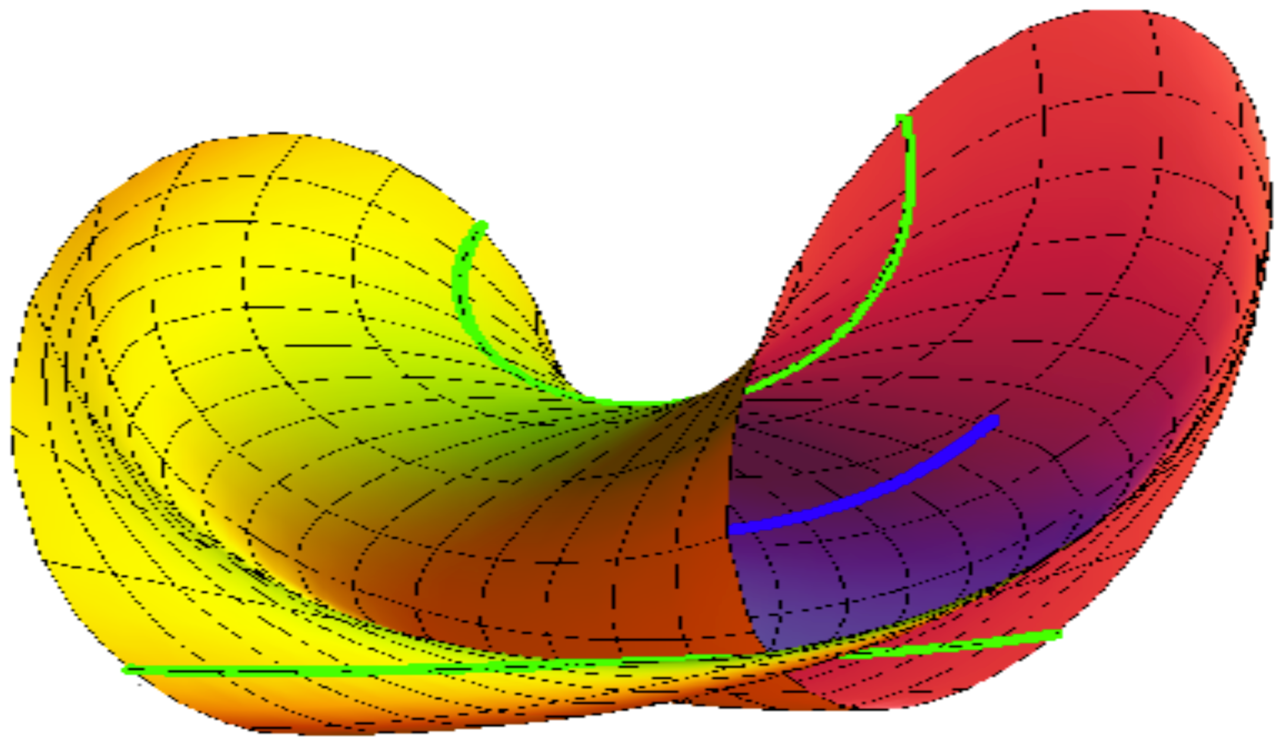
Clearly, if , then . In the case of , we have . For and , the corresponding timelike roller coaster surface with the spine curve (blue) is shown in Figure 6. Singularities appear on the striction curves (green).
4. Conclusions
This work investigates the smooth one-parameter family of standard Lorentzian circles with a fixed radius. A similar surface, named a timelike circular surface, has a fixed radius. Then, several corresponding properties of timelike circular surfaces with ruled surfaces were obtained. Through the differential operation of the frame, the geometric properties of the timelike circular surface are explained, and their geometric meanings are presented. Additionally, the conditions for timelike roller coaster surfaces to be flat or minimal surfaces are obtained. Finally, some illustrative examples were presented. Furthermore, interdisciplinary research can provide valuable new insights, but synthesizing articles across disciplines with highly varied standards, formats, terminology, and methods required an adapted approach. Recently, many interesting papers have been written related to symmetry, molecular cluster geometry analysis, submanifold theory, singularity theory, eigenproblems, etc. [17,18,19,20,21,22,23,24,25,26,27,28,29,30,31,32,33,34,35,36,37,38,39,40,41,42,43,44,45,46,47,48,49,50,51,52,53]. In future works, we plan to study the timelike circular surfaces and singularities for different queries and further improve the results in this paper, combined with the technics and results in [17,18,19,20,21,22,23,24,25,26,27,28,29,30,31,32,33,34,35,36,37,38,39,40,41,42,43,44,45,46,47,48,49,50,51,52,53]. We intend to perform the implementation of those results and explore new methods to find more results and theorems related to the symmetric properties of this topic in our following papers.
Author Contributions
Conceptualization, Y.L., F.M. and R.A.A.-B.; methodology, Y.L., F.M. and R.A.A.-B.; investigation, Y.L., F.M. and R.A.A.-B.; writing—original draft preparation, Y.L., F.M. and R.A.A.-B.; writing—review and editing, Y.L., F.M. and R.A.A.-B. All authors have read and agreed to the published version of the manuscript.
Funding
This research was funded by the National Natural Science Foundation of China (grant No. 12101168), Zhejiang Provincial Natural Science Foundation of China (grant No. LQ22A010014) and Princess Nourah bint Abdulrahman University Researchers Supporting Project number (PNURSP2022R27) of Princess Nourah bint Abdulrahman University in Riyadh, Saudi Arabia.
Institutional Review Board Statement
Not applicable.
Informed Consent Statement
Not applicable.
Data Availability Statement
Not applicable.
Acknowledgments
We gratefully acknowledge the constructive comments from the editor and the anonymous referees and Princess Nourah bint Abdulrahman University Researchers Supporting Project number (PNURSP2022R27) of Princess Nourah bint Abdulrahman University in Riyadh, Saudi Arabia.
Conflicts of Interest
The authors declare no conflict of interest.
References
- Izumiya, S.; Takeuchi, N. Singularities of ruled surfaces in 𝔼3. In Mathematical Proceedings of the Cambridge Philosophical Society; Cambridge University Press: Cambridge, UK, 2001; Volume 130. [Google Scholar]
- Izumiya, S.; Takeuchi, N. Geometry of ruled surfaces. In Applicable Mathematics in the Golden Age; Narosa Publishing House: New Delhi, India, 2003; pp. 305–338. [Google Scholar]
- Izumiya, S. Special curves and ruled surfaces. Contrib. Algebra Geom. 2003, 44, 203–212. [Google Scholar]
- Blum, R. Circles on surfaces in the Euclidean 3-space. In Geometry and Differential Geometry; Lecture Notes in Mathematics; Springer: Berlin/Heidelberg, Germany, 1980; Volume 792, pp. 213–221. [Google Scholar]
- Xu, Z.; Feng, R.; Sun, J. Analytic and algebraic properties of canal surfaces. J. Comput. Appl. Math. 2006, 195, 220–228. [Google Scholar] [CrossRef]
- Cui, L.; Wang, D.L.; Dai, J.S. Kinematic geometry of circular surfaces with a fixed radius based on Euclidean invariants. ASME J. Mech. 2009, 131, 101009. [Google Scholar]
- Izumiya, S.; Saji, K.; Takeuchi, N. Circular surfaces. Adv. Geom. 2007, 7, 295–313. [Google Scholar] [CrossRef]
- Izumiya, S.; Saji, K.; Takeuchi, N. Great circular surfaces in the three-sphere. Differ. Geom. Appl. 2011, 29, 409–425. [Google Scholar] [CrossRef]
- Gorjanc, S.; Jurkin, E. Circular surfaces CS(α, p). Filomat 2015, 29, 725–737. [Google Scholar] [CrossRef]
- Abdel-Baky, R.A.; Unluturk, Y. On the curvatures of spacelike circular surfaces. Kuwait J. Sci. 2016, 43, 50–58. [Google Scholar]
- Tuncer, O.; Canakcı, Z.; Gok, I.; Yaylı, Y. Circular surfaces with split quaternionic representations in Minkowski 3-space. Adv. Appl. Clifford Algebr. 2018, 28, 63. [Google Scholar] [CrossRef]
- Alluhaibi, N. Circular surfaces and singularities in Euclidean 3-space E3. AIMS Math. 2022, 7, 12671–12688. [Google Scholar] [CrossRef]
- Abdel-Baky, R.; Alluhaibi, N.; Ali, A.; Mofarreh, F. A study on timelike circular surfaces in Minkowski 3-space. Int. J. Geom. Methods Mod. Phys. 2020, 17, 2050074. [Google Scholar] [CrossRef]
- O’Neil, B. Semi-Riemannian Geometry with Applications to Relativity; Academic Press: New York, NY, USA, 1983. [Google Scholar]
- Mc-Nertney, L.V. One-Parameter Families of Surfaces with Constant Curvature in Lorentz Three-Space. Ph.D. Thesis, Brown University, Providence, RI, USA, 1980. [Google Scholar]
- Walrave, J. Curves and Surfaces in Minkowski Space. Ph.D. Thesis, K.U. Leuven, Faculty of Science, Leuven, Belgium, 1995. [Google Scholar]
- Sharma, J.R.; Kumar, S.; Jäntschi, L. On a class of optimal fourth order multiple root solvers without using derivatives. Symmetry 2019, 11, 1452. [Google Scholar] [CrossRef]
- Joita, D.M.; Tomescu, M.A.; Bàlint, D.; Jäntschi, L. An Application of the Eigenproblem for Biochemical Similarity. Symmetry 2021, 13, 1849. [Google Scholar] [CrossRef]
- Jäntschi, L. Introducing Structural Symmetry and Asymmetry Implications in Development of Recent Pharmacy and Medicine. Symmetry 2022, 14, 1674. [Google Scholar] [CrossRef]
- Jäntschi, L. Binomial Distributed Data Confidence Interval Calculation: Formulas, Algorithms and Examples. Symmetry 2022, 14, 1104. [Google Scholar] [CrossRef]
- Jäntschi, L. Formulas, Algorithms and Examples for Binomial Distributed Data Confidence Interval Calculation: Excess Risk, Relative Risk and Odds Ratio. Mathematics 2021, 9, 2506. [Google Scholar] [CrossRef]
- Donatella, B.; Jäntschi, L. Comparison of Molecular Geometry Optimization Methods Based on Molecular Descriptors. Mathematics 2021, 9, 2855. [Google Scholar]
- Mihaela, T.; Jäntschi, L.; Doina, R. Figures of Graph Partitioning by Counting, Sequence and Layer Matrices. Mathematics 2021, 9, 1419. [Google Scholar]
- Kumar, S.; Kumar, D.; Sharma, J.R.; Jäntschi, L. A Family of Derivative Free Optimal Fourth Order Methods for Computing Multiple Roots. Symmetry 2020, 12, 1969. [Google Scholar] [CrossRef]
- Deepak, K.; Janak, R.; Jäntschi, L. A Novel Family of Efficient Weighted-Newton Multiple Root Iterations. Symmetry 2020, 12, 1494. [Google Scholar]
- Janak, R.; Sunil, K.; Jäntschi, L. On Derivative Free Multiple-Root Finders with Optimal Fourth Order Convergence. Mathematics 2020, 8, 1091. [Google Scholar]
- Jäntschi, L. Detecting Extreme Values with Order Statistics in Samples from Continuous Distributions. Mathematics 2020, 8, 216. [Google Scholar] [CrossRef]
- Deepak, K.; Janak, R.; Jäntschi, L. Convergence Analysis and Complex Geometry of an Efficient Derivative-Free Iterative Method. Mathematics 2019, 7, 919. [Google Scholar]
- Jäntschi, L.; Bolboacă, S.D. Conformational study of C24 cyclic polyyne clusters. Int. J. Quantum Chem. 2018, 118, 25614. [Google Scholar] [CrossRef]
- Ünlütürk, Y.; Yilmaz, S. A new approach to timelike surfaces which contain inclined curves as geodesics. Differ. Equ. Dyn. Syst. 2019, 1–8. [Google Scholar] [CrossRef]
- Yang, Z.C.; Li, Y.; Erdoǧdub, M.; Zhu, Y.S. Evolving evolutoids and pedaloids from viewpoints of envelope and singularity theory in Minkowski plane. J. Geom. Phys. 2022, 176, 104513. [Google Scholar] [CrossRef]
- Li, Y.; Ganguly, D.; Dey, S.; Bhattacharyya, A. Conformal η-Ricci solitons within the framework of indefinite Kenmotsu manifolds. AIMS Math. 2022, 7, 5408–5430. [Google Scholar] [CrossRef]
- Li, Y.; Abolarinwa, A.; Azami, S.; Ali, A. Yamabe constant evolution and monotonicity along the conformal Ricci flow. AIMS Math. 2022, 7, 12077–12090. [Google Scholar] [CrossRef]
- Li, Y.; Khatri, M.; Singh, J.P.; Chaubey, S.K. Improved Chen’s Inequalities for Submanifolds of Generalized Sasakian-Space-Forms. Axioms 2022, 11, 324. [Google Scholar] [CrossRef]
- Li, Y.; Uçum, A.; İlarslan, K.; Camcı, Ç. A New Class of Bertrand Curves in Euclidean 4-Space. Symmetry 2022, 14, 1191. [Google Scholar] [CrossRef]
- Li, Y.; Mofarreh, F.; Agrawal, R.P.; Ali, A. Reilly-type inequality for the Φ-Laplace operator on semislant submanifolds of Sasakian space forms. J. Inequal. Appl. 2022, 2022, 102. [Google Scholar] [CrossRef]
- Li, Y.; Mofarreh, F.; Dey, S.; Roy, S.; Ali, A. General Relativistic Space-Time with η1-Einstein Metrics. Mathematics 2022, 10, 2530. [Google Scholar] [CrossRef]
- Li, Y.; Dey, S.; Pahan, S.; Ali, A. Geometry of conformal η-Ricci solitons and conformal η-Ricci almost solitons on Paracontact geometry. Open Math. 2022, 20, 574–589. [Google Scholar] [CrossRef]
- Li, Y.; Şenyurt, S.; Özduran, A.; Canlı, D. The Characterizations of Parallel q-Equidistant Ruled Surfaces. Symmetry 2022, 14, 1879. [Google Scholar] [CrossRef]
- Li, Y.; Haseeb, A.; Ali, M. LP-Kenmotsu manifolds admitting η-Ricci solitons and spacetime. J. Math. 2022, 2022, 6605127. [Google Scholar]
- Antić, M.; Moruz, M.; Van, J. H-Umbilical Lagrangian Submanifolds of the Nearly Kähler × . Mathematics 2020, 8, 1427. [Google Scholar] [CrossRef]
- Antić, M.; Djordje, K. Non-Existence of Real Hypersurfaces with Parallel Structure Jacobi Operator in S6(1). Mathematics 2022, 10, 2271. [Google Scholar] [CrossRef]
- Antić, M. Characterization of Warped Product Lagrangian Submanifolds in . Results Math. 2022, 77, 106. [Google Scholar] [CrossRef]
- Antić, M.; Vrancken, L. Conformally flat, minimal, Lagrangian submanifolds in complex space forms. Sci. China Math. 2022, 65, 1641–1660. [Google Scholar] [CrossRef]
- Antić, M.; Hu, Z.; Moruz, M.; Vrancken, L. Surfaces of the nearly Kähler × preserved by the almost product structure. Math. Nachr. 2021, 294, 2286–2301. [Google Scholar] [CrossRef]
- Antić, M. A class of four-dimensional CR submanifolds in six dimensional nearly Kähler manifolds. Math. Slovaca 2018, 68, 1129–1140. [Google Scholar] [CrossRef]
- Antić, M. A class of four dimensional CR submanifolds of the sphere S6(1). J. Geom. Phys. 2016, 110, 78–89. [Google Scholar] [CrossRef]
- Ali, A.T. Non-lightlike constant angle ruled surfaces in Minkowski 3-space. J. Geom. Phys. 2020, 157, 103833. [Google Scholar] [CrossRef]
- Ali, A.T. A constant angle ruled surfaces. Int. J. Geom. 2018, 7, 69–80. [Google Scholar]
- Ali, A.T. Non-lightlike ruled surfaces with constant curvatures in Minkowski 3-space. Int. J. Geom. Methods Mod. Phys. 2018, 15, 1850068. [Google Scholar] [CrossRef]
- Ali, A.T.; Hamdoon, F.M. Surfaces foliated by ellipses with constant Gaussian curvature in Euclidean 3-space. Korean J. Math. 2017, 25, 537–554. [Google Scholar]
- Ali, A.T.; Abdel Aziz, H.S.; Sorour, A.H. On some geometric properties of quadric surfaces in Euclidean space. Honam Math. J. 2016, 38, 593–611. [Google Scholar] [CrossRef]
- Ali, A.T.; Abdel Aziz, H.S.; Sorour, A.H. On curvatures and points of the translation surfaces in Euclidean 3-space. J. Egyptian Math. Soc. 2015, 23, 167–172. [Google Scholar] [CrossRef] [Green Version]
Figure 1.
A cross-section of M.

Figure 2.
has a cusp at .

Figure 3.
M has different singular points.

Figure 4.
M has different singular points along the striction curves.

Figure 5.
M has different singular points.

Figure 6.
Timelike roller coaster surface with its spine and striction curves.

Publisher’s Note: MDPI stays neutral with regard to jurisdictional claims in published maps and institutional affiliations. |
© 2022 by the authors. Licensee MDPI, Basel, Switzerland. This article is an open access article distributed under the terms and conditions of the Creative Commons Attribution (CC BY) license (https://creativecommons.org/licenses/by/4.0/).
Share and Cite
MDPI and ACS Style
Li, Y.; Mofarreh, F.; Abdel-Baky, R.A. Timelike Circular Surfaces and Singularities in Minkowski 3-Space. Symmetry 2022, 14, 1914. https://doi.org/10.3390/sym14091914
AMA Style
Li Y, Mofarreh F, Abdel-Baky RA. Timelike Circular Surfaces and Singularities in Minkowski 3-Space. Symmetry. 2022; 14(9):1914. https://doi.org/10.3390/sym14091914
Chicago/Turabian StyleLi, Yanlin, Fatemah Mofarreh, and Rashad A. Abdel-Baky. 2022. "Timelike Circular Surfaces and Singularities in Minkowski 3-Space" Symmetry 14, no. 9: 1914. https://doi.org/10.3390/sym14091914
Note that from the first issue of 2016, this journal uses article numbers instead of page numbers. See further details here.