Obstacle Avoidance Path Planning of Space Robot Based on Improved Particle Swarm Optimization

Abstract

In order to meet security requirements of space on orbit service, an obstacle avoidance trajectory planning method using improved particle swarm optimization had been presented in this paper. On the basis of the actual overall structure of 7 degrees of freedom redundant space manipulator and the characteristics of obstacles, the envelope method was used to model the arm and obstacles, respectively. The limit conditions to avoid the collision between them were analyzed. Then, the fitness function under the symmetrical conditions of avoiding the collision and searching for the shortest trajectory was constructed. In addition, the obstacle avoidance trajectory planning was solved based on improved particle swarm optimization (IPSO). Finally, simulation experiments were carried out to prove its effectiveness and rationality, where there were symmetrical advantages in two aspects. It can be concluded that the presented method based on IPSO has strong robustness.

1. Introduction

When a space robot performs an operational mission in space, it needs to avoid some of its own equipment or obstacles during its movement [1]. Therefore, to complete space on orbit service successfully, it is not only necessary but also very important to study and explore the obstacle avoidance method. The obstacle avoidance path planning refers to search for a trajectory, which should comply with the symmetrical two points, that is the starting position to the target location. It should also avoid obstacles. In addition, it needs to meet some specific conditions [2].

For the obstacle avoidance problem, many researchers and scholars have explored and put forward different solutions. Nowadays, group intelligent optimization algorithms are used more and more frequently in the problem of obstacle avoidance [3]. In general, the methods define guidelines related to path planning, such as minimum torque, optimal energy, and speed limitations, which differ from each other in the description of objective optimization function and in the solution process of group intelligence optimization algorithms [4]. For example, M.G. Marcos and others proposed a closed-loop broad inverse path planning method using GA, which was to search the optimal value in joint space. The constraints of the target function included the position error of end executor under the Descartes coordinate system, the velocity and acceleration of joint angle and so on [5]. A. Shukla and others proposed a method which converted the problem into a solution to make all joints move in the complete path set and minimize the amount of movement of all joints [6]. The mathematical probability method [7] referred to the construction of vector diagrams between the initial and target point locations, solving obstacle avoidance path planning problems through the nodes of vector graph, such as the rapid expansion of random tree method [8] and the probability map method [9]. Path smoothing methods include the B-Se like curve method and segment interpolation method [10], etc.

The above obstacle avoidance methods have both advantages and disadvantages in solving the problem. The advantage is that it could settle the problem of obstacle avoidance under certain constraints, whereas the disadvantage is that the robustness is poor. In the complex space environment, it is difficult to search for collision-free paths that meet the constraints, especially to find relatively short collision-free paths. To get a shorter collision-less path and improve the robustness of the obstacle avoidance method, an obstacle avoidance path planning method based on IPSO was presented. First of all, transforming the actual collision problem into a mathematical problem that can be quantified; a spherical envelope method was adopted to model obstacles. The actual overall structure of the space robot was considered. The simplified model adopted the cylindrical envelope method, and the various limit conditions in the event of collision between models were analyzed. The anti-collision space was constructed. The obstacle avoidance problem of 3D space was symmetrically transformed into 2D through one-to-one mapping. Then, the fitness function was established. To search the shorter obstacle avoidance path and enhance robustness, an obstacle avoidance path planning method based on IPSO was presented. Finally, the proposed method was compared with the method based on PSO through the simulation experiment.

2. Construction of Anti-Collision Space

2.1. Establishment of Simplified Model

To solve the obstacle avoidance problem, it is more important to solve the problem of the obstacle and arm model. Common modeling methods for obstacles and arm rods include the grid method [11], the unit tree method [12], and the polygon method [13], etc.

In this paper, the polygonal method was adopted to model these obstacles, and the obstacles were enveloped with geometric spherical shapes in 3D space [14]. Although the obstacles after modeling is bigger than the actual obstacle, it improves the safety performance and the calculation is more convenient. Each link of a 7 degrees of freedom redundant space robot can be simplified into a cylinder. In order to improve the flexibility of a space robot, the 7 degrees of freedom adopts rotating joints. The central axes of the first two joints are perpendicular to each other. The central axes of the third joint and fourth joint are perpendicular to each other. The adjacent central axes of last four joints are perpendicular to each other. The three end rotating joints form a spherical joint as the wrist joint of the manipulator. The axes of the two rotating joints are parallel to each other and can intersect on the center point of the middle joint axis. The shoulder joint and elbow joint are connected together. The wrist and elbow joints are connected by rigid bodies. The cube model and cylinder model of 3D space are symmetrically mapped to a 2D space model, as described in Figure 1.

In Figure 1, the red area represents the obstacle model. The blue area represents the connecting rod model of a 7 degrees of freedom redundant space robot.

2.2. Collision Analysis

Based on the establishment of the obstacle model and the 7 degrees of freedom redundant space robot link model, it can be concluded that there are a total of three spatial relationships between the two models [15]. These are separation, tangency, and intersection. The two can avoid collisions when the obstacle model is parted or cut off from the connecting rod model.

Many methods of collision avoidance were proposed by researchers at home and abroad. According to the method of model establishment, this paper analyzed whether the arm and obstacle collide by judging the space among the control points of the arm and the center of obstacles.

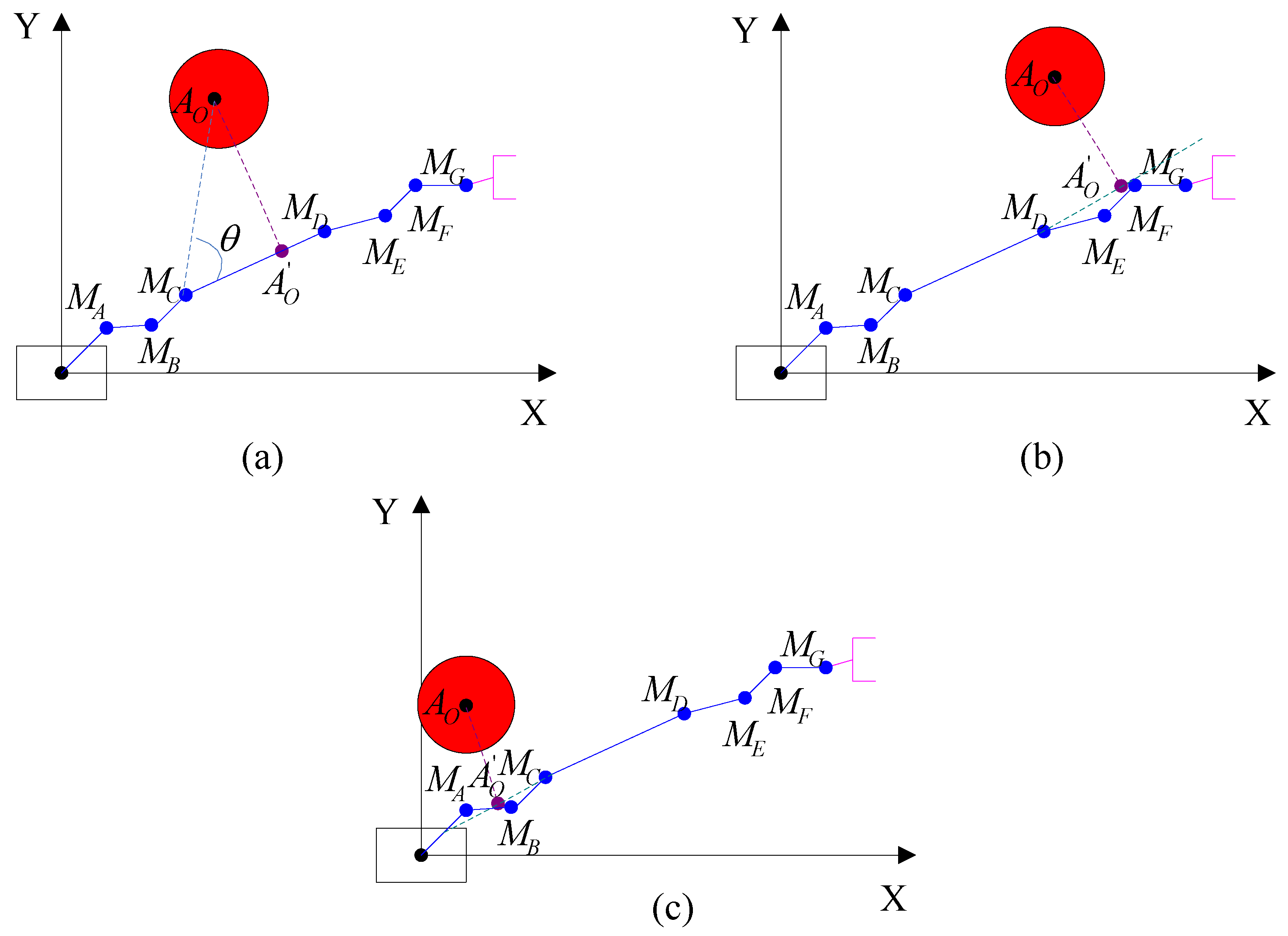
The collision relationship between an obstacle and an arm was mathematically expressed as shown in Figure 2.

In Figure 2, the collision analysis between obstacles and 7 degrees of freedom redundant space robots can be converted into the center of the obstacle, the projection, and the relationship between the control points. Where, $\mathcal{O}$ represents the origin of the coordinate system, $M_A-M_G$ represents the center point of seven joints separately, $A_O$ represents the center of obstacles, $A_R$ represents the radius of the obstacle model, and $A_O^{{}^{\prime }}$ represents the projection of obstacles’ center.

Take the link $M_C{M}_D$ as an example to analyze its relationship with obstacles. In the actual solution process, each connecting rod uses this method to determine whether there is a collision with the obstacle. Firstly, the two endpoints of the connecting rod $M_C{M}_D$ are considered to be fixed control points. In order to prevent a collision between the connecting rod and obstacles, the following conditions need to be met, as shown in Formula (1).

$$\left\{\begin{array}{c}\left|A_O{M}_C\right|⩾A_R\\ \left|A_O{M}_D\right|⩾A_R\end{array}\right.$$

(1)

There are three types of relationships between the projection $A_O^{{}^{\prime }}$ and the connecting rod $M_C{M}_D$, as shown in Figure 3.

As can be seen from Figure 3, the projection of obstacles’ center can be on the connecting rod, on the right extension line, or on the left extension line. Where, $\theta$ represents a joint or the corner of a joint.

When the projection $A_O^{{}^{\prime }}$ is on a connecting rod, the following conditions need to be met, as shown in Formula (2).

$$\left|A_O{M}_C\right|·cos\theta ⩽\left|M_C{M}_D\right|$$

(2)

At this time, $A_O^{{}^{\prime }}$ is regarded as a control point of the connecting rod $M_C{M}_D$, that is to prevent a collision between the connecting rod and the obstacle, the following conditions need to be met, as shown in Formula (3).

$$\left|A_O{A}_O^{{}^{\prime }}\right|⩾A_R$$

(3)

When the projection $A_O^{{}^{\prime }}$ is on the symmetrical right or left extension line of the connecting rod, $A_O^{{}^{\prime }}$ is not the control point of connecting rod $M_C{M}_D$. In general, there are three or two control points for a link. There are two fixed control points and one flexible control point. When the center of the obstacle is projected on the link, there are three control points. So that no incident occurs between the link and obstacle, it should meet Formulas (1) and (3). When the center of the obstacle is projected on the extension line on the right or left side of the connecting rod, there are two control points. So that no incident occurs between the link and obstacle, Formula (1) needs to be met.

2.3. Establishment of the Fitness Function

The fitness function refers to that under certain constraint conditions, the space manipulator could travel from the starting position to the target position without any collision. In addition, the path planning should be as short as possible. The specific expression of the obstacle avoidance fitness function is as shown in Formula (4).

$$c_1\left(\theta \right)⩽0, c_2\left(\theta \right)⩽0\min F\left(\theta \right)={\omega }_1{\mathit{f}}_1\left(\theta \right)+{\omega }_2{\mathit{f}}_2\left(E_p\right)+{\omega }_3{\mathit{f}}_3\left(\theta \right)$$

(4)

where, $c_1\left(\theta \right)$ and $c_2\left(\theta \right)$ represent the constraints of the fitness function; $\theta$ represents joint angles or complement angles; ${\mathit{f}}_1\left(\theta \right)$ represents the first part of the fitness function to be optimized; $E_p$ represents the current position of the end effector; ${\mathit{f}}_2\left(E_p\right)$ represents the second part of the fitness function; ${\mathit{f}}_3\left(\theta \right)$ represents the third part of the fitness function; ${\omega }_1$, ${\omega }_2$ and ${\omega }_3$ represent the weight coefficient, respectively, ${\omega }_1+{\omega }_2+{\omega }_3=1$, ${\omega }_1\in [0,1]$, ${\omega }_2\in [0,1]$, ${\omega }_3\in [0,1]$, ${\omega }_1$ is more important than ${\omega }_2$ and ${\omega }_3$. Because the function ${\mathit{f}}_1\left(\theta \right)$ takes up more proportions than ${\mathit{f}}_2\left(E_p\right)$ and ${\mathit{f}}_3\left(\theta \right)$, and ${\omega }_1>({\omega }_2={\omega }_3)$.

A specific analysis has been described above. It is in this way that the fixed control points of the 7 degrees of freedom redundant space robot arm lever can be kept away from obstacles, as shown in Formula (5).

$${\mathit{f}}_1\left(\theta \right)=\sum _{p_i=1}^{p_n}\sum _{A_i=1}^{A_n}{E}_d\left(\theta \right)\left\{M_{P_i,A_{O,i}}\right\}$$

(5)

where, $A_i$ and $P_i$ represent the number of variables; $P_n$ represents the amount of fixed control points; $A_n$ represents a quantity of obstacles; $M_{P_i}$ represents a fixed control point, that is the center point of each joint of a 7 degrees of freedom redundant space robot; $A_{O,i}$ shows the center point of an obstacle model; $E_d\left(\theta \right)\left\{M_{P_i},A_{O,i}\right\}$ represents the European space between a fixed control point and the center of an obstacle model.

The exact expression of the end effector traveling to the goal point from the starting point should be as shown in Formula (6).

$${\mathit{f}}_2\left(E_P\right)=\sqrt{{(x-x_g)}^2+{(y-y_g)}^2+1}$$

(6)

where, $(x_g,y_g)$ represents the goal point position of the end-effector.

The exact expression of distance from the goal point to the end-effector is as shown by Formula (7).

$${\mathit{f}}_3\left(\theta \right)=∥L\left(\theta \right)∥$$

(7)

where, $L\left(\theta \right)$ indicates the distance from the goal point to the end-effector; $∥x∥$ indicates the bound norm, and $∥x∥=\sqrt{x^{T}x}$.

The constraints include two types. One is for the constraints of the 7 degrees of freedom redundant space robot, including joint, joint speed and joint acceleration, and the other is for the end effector away from obstacles and flexible control points.

The constraints of joint, joint speed, and joint acceleration of a 7 degrees of freedom redundant space robot are expressed as shown in Formulas (8) and (9).

$${\theta }_{i\min }⩽{\theta }_i⩽{\theta }_{i\max }i=1, 2, \dots , 7$$

(8)

$$|{\dot{\theta }}_i\left(t\right)|⩽1 \mathrm{rad}/\mathrm{s}|{\ddot{\theta }}_i\left(t\right)|⩽1 \mathrm{rad}/{\mathrm{s}}^2$$

(9)

where, ${\theta }_i$ represents the value of a joint; ${\theta }_{i\min }$ represents the minimum value of a joint; ${\theta }_{i\max }$ indicates the maximum value of a joint; ${\dot{\theta }}_i\left(t\right)$ represents the velocity of a joint; and ${\ddot{\theta }}_i\left(t\right)$ represents the acceleration of a joint.

During the obstacle avoidance movement of a 7 degrees of freedom redundant space robot, its end effector should be kept away from the obstacle. The Euclidean distance from the end effector to the center of the obstacle model is greater than its radius, as shown in Formula (10).

$$A_R-E_d\left\{E_P,A_O\right\}⩽0$$

(10)

where, $A_R$ represents the radius of the obstacle model; $E_d\left\{E_P,A_O\right\}$ represents the Euclidean distance, which is from the end-effector to the center of the obstacle model.

The constraint analysis of flexible control points away from obstacles is described above, as shown in Formula (11).

$$A_R-E_d\left\{A_{O,i}^{{}^{\prime }},A_{O,i}\right\}⩽0$$

(11)

where, $A_{O,i}^{{}^{\prime }}$ represents the projection; $E_d\left\{A_{O,i}^{{}^{\prime }},A_{O,i}\right\}$ represents the Euclidean distance, which is from the projection to the center point of the obstacle model.

3. Obstacle Avoidance Path Planning Based on IPSO

3.1. Particle Swarm Optimization

In the magical natural world, all kinds of creatures have their own laws of existence and evolution. Particle Swarm Optimization (PSO) was first summarized by Dr. Eberhart and Dr. Kennedy [16]. During the flight of birds in nature, the birds will slowly move closer to the direction of food, and the actions of the group are consistent [17]. However, individual birds may suddenly change direction. It is found that there are similar phenomena and laws in other group organisms, which is the mechanism of sharing and mutation between groups. It is beneficial to the development of the whole population. In the process of evolution, particles have no mass and volume, equivalent to a bird in a flock, and the solution is equivalent to a food source.

In recent years, the applications of PSO have been very wide, which is due to its advantages. It has the advantage of a simple structure, it is easy to understand and it has less parameters [18]. In the PSO, each particle is expressed and described by speed and position. The rules of an evolutionary process are determined by the fitness function values. The ith particle can be expressed in a vector, as shown in Formula (12).

$$Z=(v_{ij},x_{ij},p_{ij})$$

(12)

where, $v_{ij}$ represents the speed of particle evolution; $x_{ij}$ represents the position of particles in evolution; $p_{ij}$ represents the optimal position of itself in particle evolution; and $j=1, 2, \dots , D$, D indicates the dimension of the solution to be optimized.

When a particle discovers during iteration that the value of its optimal position is greater than the value of the global optimal position, it moves toward the global optimal position. Throughout the search, particles constantly update their speed and position. Its equations are as shown in Formula (13).

$$\left\{\begin{array}{c}{v}_{ij}^{t+1}=w{v}_{ij}^t+c_1{r}_1[p_{ij}-x_{ij}^t]+c_2{r}_2[p_{gj}-x_{ij}^t]\\ x_{ij}^{t+1}=x_{ij}^t+v_{ij}^{t+1}\end{array}\right.$$

(13)

where, w represents the inertial weight of a particle; $c_1$ and $c_2$ represent the learning factor of a particle; $r_1$ and $r_2$ represent a value among $[0,1]$ randomly; and $p_{gj}$ represents the optimal position in population evolution.

3.2. Obstacle Avoidance Path Planning Based on IPSO

PSO has the advantages of being simple and easy to operate. However, like other algorithms, it also has its own inevitable disadvantages. For example, it has poor robustness and low solution accuracy. To improve the defects of PSO in solving complex problems, an improved particle swarm algorithm (IPSO) [19] has been adopted to optimize the problem of obstacle avoidance path planning. IPSO has three populations. Population 1 and 2 were optimized in the same way, and Population 3 depended on them. To some extent, it overcomes the shortcomings of PSO. In Population 1 and 2, the velocity and position are renewed through Formula (13). The description of inertia weight is in Formula (14).

$$w=w_{\max }-\frac{\left(w_{\max }-w_{\min }\right)}{M}t$$

(14)

where, $w_{\max }$ is the maximum value; $w_{\min }$ is the minimum value; and M is the maximum iterations.

The velocity in Population 3 is renewed through Population 1 and 2, which was as shown in the literature [19].

Based on the method of improving the particle group algorithm, the specific simulation experiment steps to optimize the problem of an obstacle avoidance path are as follows.

• Set the parameters, including the parameters of improved particle swarm optimization, obstacles and 7 degrees of freedom redundant space robot.
• Initialize the velocity and position of particles, which are stochastic under constraints.
• Calculate the fitness function value in each population by Formula (4).
• Update the velocity and position in each population.
• Compare the present position of all particles themselves with the former optimal positions. If they were well, update their own best positions. Conversely, retain the former optimal position.
• Compare all current $p_{ij}$ and $p_{gj}$, and update $p_{gj}$.
• Meet the number of iterations to determine the shortest collision-free path.

4. Simulation Experiments and Discussion

The simulation experiments were carried out to prove the effectiveness and rationality of the proposed method. The 7 degrees of freedom redundant space robot was used as the research object. It was on the MATLB platform, compared with the method using PSO.

To make a fair comparison, the number of simulation experiments per group was set to 20. The minimum, maximum, average, and percentage of simulation results that reach the threshold of 4.33 need to be recorded.

In this simulation, three different obstacles were randomly set. The parameter coordinates are followed by $(0.5,0.5,0)$, $(0.4,0.7,0)$ and $(0.2,0.8,0)$. The position of the start point is $(0,1.336,0)$. The position of the end point is $(0.7,0.3,0)$. The parameter setting of two points is according to the 7 degrees of freedom redundant space robot.

The weight factor in the fitness function is ${\omega }_1=0.5$, ${\omega }_2={\omega }_3=0.25$, which had been explained in the above Formula (4).

The proposed method in this paper has no specific requirements for the initial attitude and target point of base. The following simulation experiments assume that the initial attitude is 0. The description of specific parameter settings are as follows, which had been explained in the literature [20].

$Q_{b0}$ is the initial posture and $Q_{bd}$ is the expected posture of the base, which are equal. The specific expression is $Q_{b0}$ = $Q_{bd}$ = ${\left[1000\right]}^T$.

${\theta }_{i\max }$ and ${\theta }_{i\min }$ has been described in Section 2.3. The range of each joint is

${\theta }_{i\max }=\pi \left[\frac{8}{9}\frac{1}{9}1\frac{17}{18}\frac{1}{9}\frac{1}{9}1\right]\left(\mathrm{rad}\right)$,

${\theta }_{i\min }=\pi \left[\frac{8}{9}\frac{1}{9}1\frac{5}{6}1\frac{23}{90}\frac{4}{9}\right]\left(\mathrm{rad}\right)$.

${\dot{\theta }}_i\left(t\right)$ is the value of joint velocity. ${\ddot{\theta }}_i\left(t\right)$ is the value of joint acceleration. The specific expressions are $|{\dot{\theta }}_i\left(t\right)|⩽1\mathrm{rad}/\mathrm{s}$ and $|{\ddot{\theta }}_i\left(t\right)|⩽1\mathrm{rad}/{\mathrm{s}}^2$.

4.1. Obstacle Avoidance Simulation Using PSO

Because this problem is complex, the number of particles is relatively large. The dimension is the number of DOF. The inertia weight and learning factors are values in the usual sense. The parameter settings are described in

Table 1. Parameter settings of PSO.

Number of Particles	Dimension	Learning Factor 1	Learning Factor 2	Inertia Weight	Maximum Number of Iterations
300	7	2	2	0.5	100

, which are of PSO.

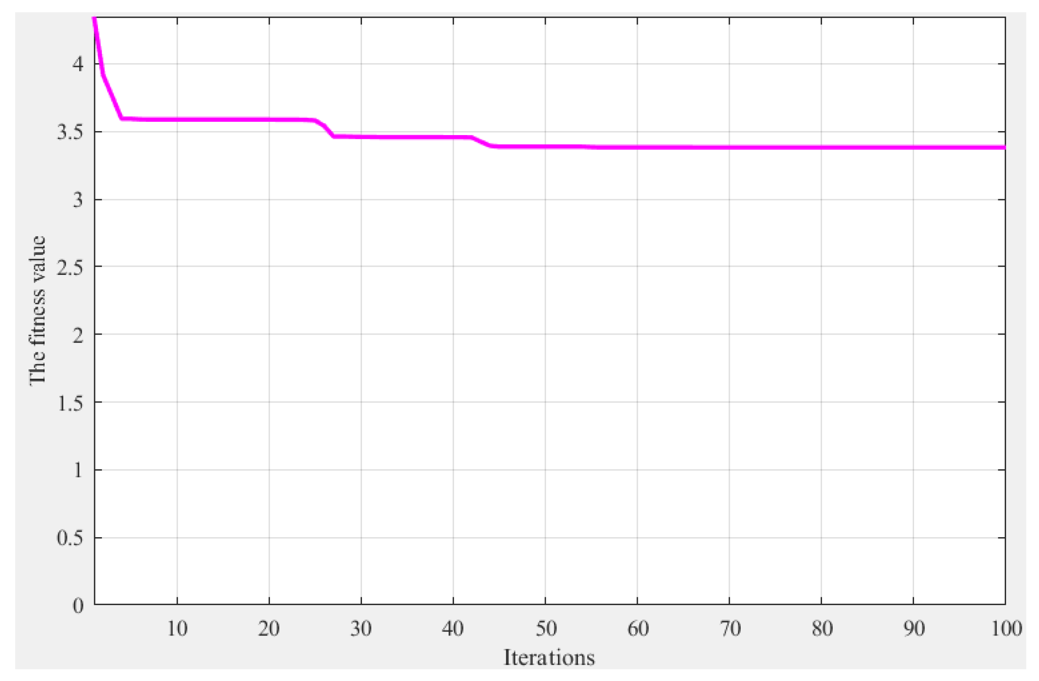
The fitness function value obtained by the method using PSO changing with the number of iterations was as shown in Figure 4.

The changes of each joint with the iterations obtained by PSO were shown in Figure 5. In addition, an obstacle avoidance path obtained by the method using PSO was as shown in Figure 6.

4.2. Obstacle Avoidance Simulation Using IPSO

In order to compare fairly, the parameter settings are described in

Table 2. Parameter settings of IPSO.

Number of Particles	Dimension	Learning Factor 1	Learning Factor 2	Maximum Inertia Weight	Minimum Inertia Weight	Maximum Number of Iterations
300	7	2	2	0.9	0.4	100

, which are of IPSO.

The fitness function value obtained by the method using IPSO changing with the number of iterations was as shown in Figure 7.

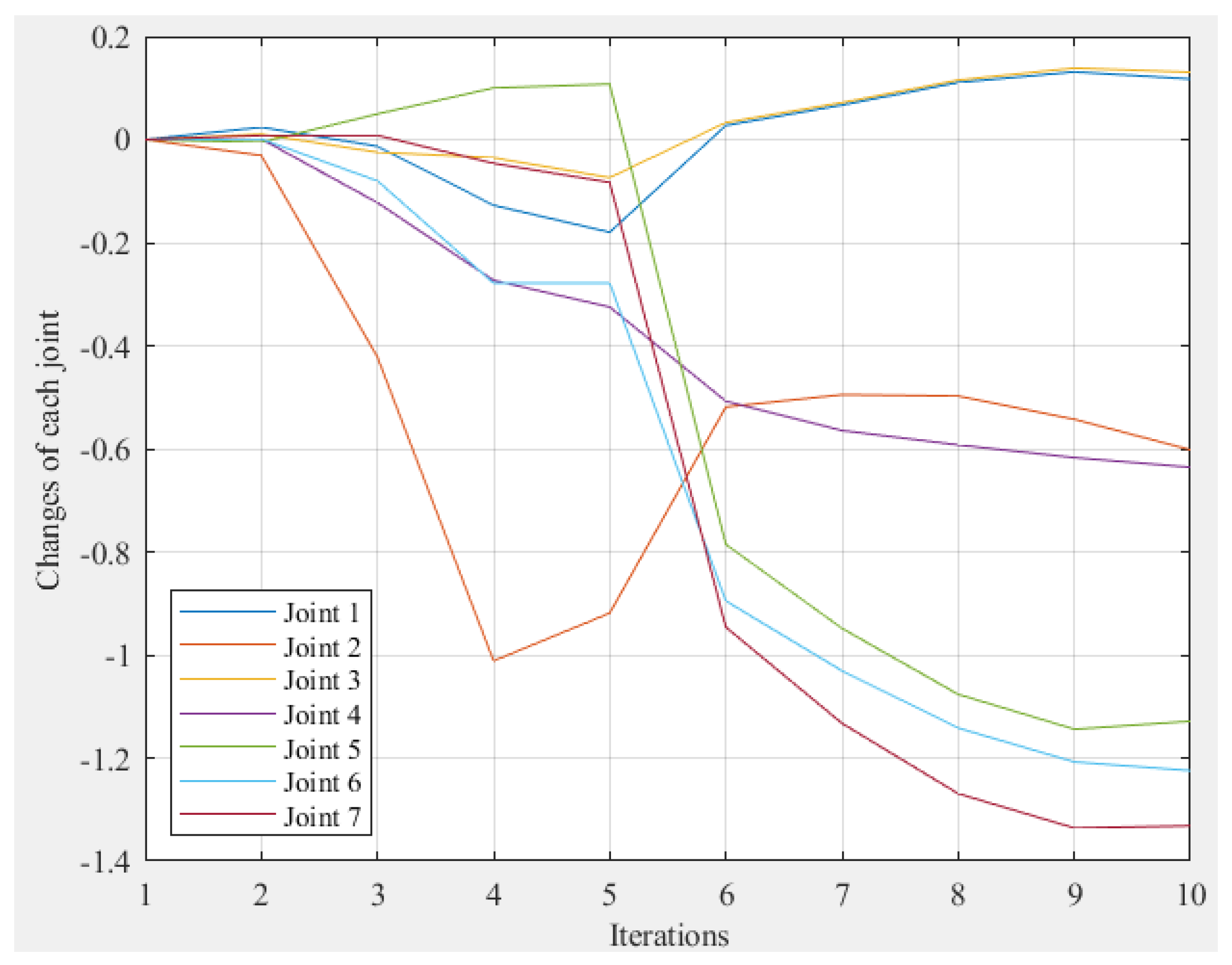
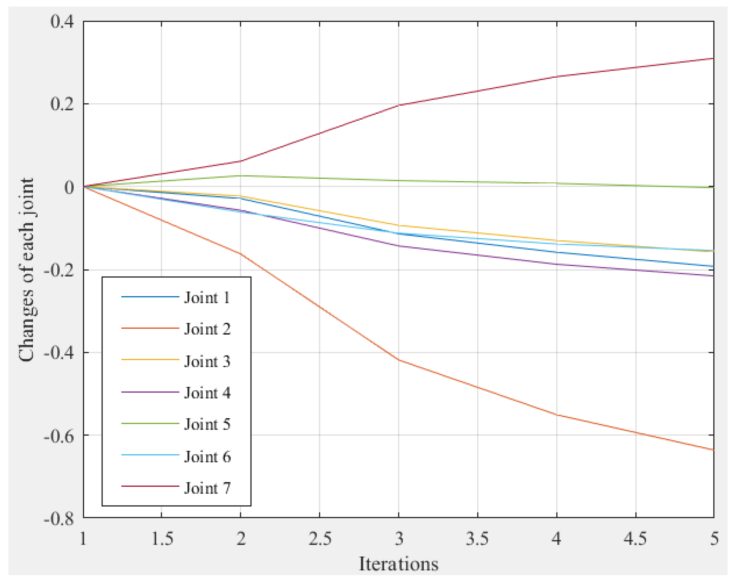
The changes of each joint with the iterations that obtained by IPSO were shown in Figure 8.

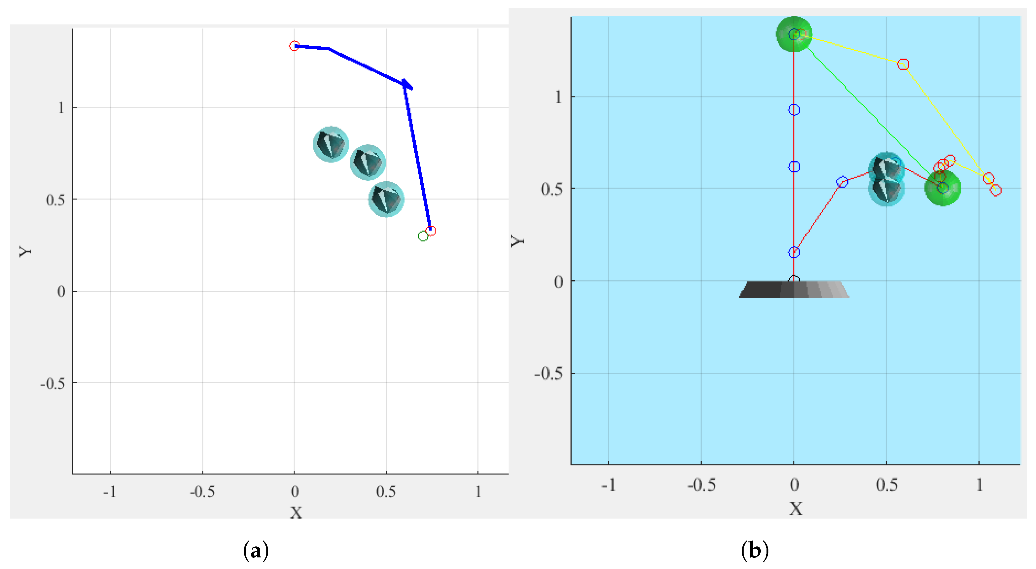
An obstacle avoidance path obtained by the method using IPSO was as shown in Figure 9.

4.3. Comparison and Discussion

Figure 4 and Figure 7 are variation diagrams, which demonstrate how the fitness function values changed with the number of iterations based on two different methods. With the increasing number of iterations, the fitness function values gradually decrease until convergence. It can be concluded that the fitness function value obtained by the method using PSO is 3.3818. However, the fitness function value obtained by the proposed method using IPSO is 3.3771 through the simulation experiments. From the fitness function value, it follows that the proposed method using IPSO is more suitable for solving the problem on obstacle avoidance trajectory planning. From Figure 5 and Figure 8, it can be shown that the changes of each joint are smoother using IPSO.

In Figure 6 and Figure 9, the blue transparent circles represent obstacles. The two red circles represent the start and end positions of the end effector. The green circle represents the position of the target point. The blue line represents the planned obstacle avoidance trajectory. It is obvious that the obstacle avoidance trajectory obtained by the proposed method based on IPSO is shorter than that obtained by the method based on PSO, which shows that the proposed method using IPSO is more effective.

The simulation experiments were symmetrically applied twenty times. The threshold rate refers to a percentage. It is a ratio that times reaching the threshold to 20 times. The results were written down as shown in

Table 3. Statistic results.

Methods	Worst Value	Optimal Value	Average Value	To Threshold Ratio
Method using PSO	4.3341	3.3818	4.2378	70%
Proposed method using IPSO	4.3296	3.3760	3.7699	100%

. In the table, the bold indicates better results.

In Table 3, the bold indicates better results. It is obvious that the worst values, optimal values and average values obtained by the proposed method based on IPSO are better than the results obtained by the method using PSO. It is shown that the proposed method based on IPSO is even better for solving the problem on obstacle avoidance trajectory planning of the 7 degrees of freedom redundant space robot. Furthermore, it can search a shorter obstacle avoidance trajectory.

A comparison of the simulation results obtained by the method based on PSO showed that the threshold ratio reached by the proposed method based on IPSO is higher, which demonstrates that the proposed method based on IPSO has better robustness.

5. Conclusions

In this paper, considering the safety of the space orbit service, the method using IPSO was proposed for the problem on obstacle avoidance path planning of the 7 degrees of freedom redundant space robot. A mathematical expression of the obstacle avoidance trajectory planning problem of the 7 degrees of freedom redundant space robot had been constructed. In order to improve the poor robustness of PSO, IPSO was adopted to optimize it. Its symmetrical effectiveness and rationality were confirmed by the simulation. The proposed obstacle avoidance trajectory planning method using IPSO included the model establishment of the 7 degrees of freedom redundant space robot and obstacle, anti-collision analysis and description of fitness function that meet the collision-free and shortest path. By comparing the simulation experiment results, it is obvious that the trajectory snuffed out by the proposed path planning method is more robust and appropriate to solve the problem on obstacle avoidance path planning of the 7 degrees of freedom redundant space robot.

References

- Sabatini, M.; Volpe, R.; Palmerini, G.B. Centralized visual based navigation and control of a swarm of satellites for on-orbit servicing. Acta Astronaut. 2020, 171, 323–334. [Google Scholar] [CrossRef]
- Jing, Z.L.; Qiao, L.F.; Pan, H.; Yang, Y.; Chen, W. An overview of the configuration and manipulation of soft robotics for on-orbit servicing. Sci. China Inf. Sci. 2017, 60, 050201. [Google Scholar] [CrossRef]
- Xiang, W.W.K.; Yan, S.Z. Dynamic analysis of space robot manipulator considering clearance joint and parameter uncertainty: Modeling, analysis and quantification. Acta Astronaut. 2020, 169, 158–169. [Google Scholar] [CrossRef]
- Zong, L.J.; Emami, M.R. Concurrent base-arm control of space manipulators with optimal rendezvous trajectory. Aerosp. Sci. Technol. 2020, 100, 105822. [Google Scholar] [CrossRef]
- Maria, D.G.M.; Tenreiro Machado, J.A.; Azevedo-Perdicoulis, T.P. Trajectory planning of redundant manipulators using genetic algorithm. Commun. Nonlinear Sci. Numer. Simul. 2009, 14, 2858–2869. [Google Scholar]
- Ashwini, S.; Ekta, S.; Pankaj, W.; Dasgupta, B. A direct variational method for planning monotonically optimal paths for redundant manipulators in constrained workspaces. Robot. Auton. Syst. 2013, 61, 209–220. [Google Scholar]
- Qian, Y.J.; Yuan, J.J.; Wan, W.W. Improved trajectory planning method for space robot-system with collision prediction. J. Intell. Robot. Syst. 2020, 99, 289–302. [Google Scholar] [CrossRef]
- Gildardo, S.; Jean-Claude, L. On delaying collision checking in PRM planning: Application to multi-robot coordination. Int. J. Robot. Res. 2002, 21, 5–26. [Google Scholar]
- Machmudah, A.; Parman, S.; Zainuddin, A.; Chacko, S. Polynomial joint angle arm robot motion planning in complex geometrical obstacles. Appl. Soft Comput. 2013, 13, 1099–1109. [Google Scholar] [CrossRef]
- Jia, Q.X.; Yuan, B.N.; Chen, G.; Fu, Y. Kinematic and dynamic characteristics of the free-floating space manipulator with free-swinging joint failure. Int. J. Aerosp. Eng. 2019, 2019, 2679152. [Google Scholar] [CrossRef] [Green Version]
- Das, P.K.; Behera, H.S.; Panigrahi, B.K. A hybridization of an improved particle swarm optimization and gravitational search algorithm for multi-robot path planning. Swarm Evol. Comput. 2016, 28, 14–28. [Google Scholar] [CrossRef]
- Zhang, B.S.; Song, B.W.; Jiang, J.; Mao, Z.Y. Optimal design of hydraulic support landing platform for a four-rotor dish-shaped UUV using particle swarm optimization. Int. J. Naval Archit. Ocean Eng. 2016, 8, 475–486. [Google Scholar] [CrossRef] [Green Version]
- Li, T.G.; Li, Q.H.; Li, W.X. A path planning algorithm for space manipulator based on Q-Learning. In Proceedings of the 2019 IEEE 8th Joint International Information Technology and Artificial Intelligence Conference, Chongqing, China, 24–26 May 2019; pp. 1566–1571. [Google Scholar]
- Tchon, K.; Respondek, W.; Ratajczak, J. Normal forms and configuration singularities of a space manipulator. J. Intell. Robot. Syst. 2019, 93, 621–634. [Google Scholar] [CrossRef]
- Piotrowski, A.P.; Napiorkowski, J.J. Searching for structural bias in particle swarm optimization and differential evolution algorithms. Swarm Intell. 2016, 10, 307–353. [Google Scholar] [CrossRef] [Green Version]
- Wang, C.; Liu, Y.C.; Chen, Y.; Wei, Y. Self-adapting hybrid strategy particle swarm optimization algorithm. Soft Comput. 2016, 20, 4933–4963. [Google Scholar] [CrossRef]
- Wang, M.M.; Luo, J.J.; Walter, U. Trajectory planning of free-floating space robot using particle swarm optimization. Acta Astronaut. 2015, 112, 77–88. [Google Scholar] [CrossRef]
- Xie, Y.E.; Wu, X.D.; Shi, Z.; Wang, Z.; Sun, J.; Hao, T. The path planning of space manipulator based on Gauss-Newton iteration method. Adv. Mech. Eng. 2017, 9, 1–12. [Google Scholar] [CrossRef]
- Zhang, J.X.; Zhang, J.X.; Zhang, F.; Chi, M.; Wan, L. An Improved Symbiosis Particle Swarm Optimization for Solving Economic Load Dispatch Problem. J. Electr. Comput. Eng. 2021, 2021, 8869477. [Google Scholar] [CrossRef]
- Zhou, D.S.; Wang, L.; Zhang, Q. Obstacle avoidance planning of space manipulator end-effector based on improved ant colony algorithm. SpringerPlus 2016, 5, 509. [Google Scholar] [CrossRef] [Green Version]
Figure 1.
2D space model diagram.
Figure 2.
Mathematical model.
Figure 3.
A circular heart projection of an obstacle. (a) On the connecting rod. (b) On the right extension line. (c) On the left extension line.
Figure 4.
Iterative variation using PSO.
Figure 5.
Changes of each joint using PSO.