
Application of Einstein Function on Bi-Univalent Functions Defined on the Unit Disc


1
Department of Mathematics, Faculty of Science, Zagazig University, Zagazig 44519, Egypt
2
Department of Mathematics, Faculty of Science, Tanta University, Tanta 31527, Egypt
3
Department of Basic Sciences, Common First Year, King Saud University, Alriyad 11451, Saudi Arabia
*
Author to whom correspondence should be addressed.
Symmetry 2022, 14(4), 758; https://doi.org/10.3390/sym14040758
Submission received: 21 March 2022
/
Revised: 1 April 2022
/
Accepted: 3 April 2022
/
Published: 6 April 2022
(This article belongs to the Special Issue Geometric Function Theory and Special Functions)
Abstract
:Motivated by q-calculus, we define a new family of , which is the family of bi-univalent analytic functions in the open unit disc U that is related to the Einstein function . We establish estimates for the first two Taylor–Maclaurin coefficients , , and the Fekete–Szegö inequality for the functions that belong to these families.
Keywords:
analytic function; Einstein function; bernoulli numbers; bi-univalent function; quantum calculus; subordinationMSC:
30C45; 30C55; 11B681. Introduction and Basic Concepts
Let denote the family of functions f normalized by
which are analytic and univalent in the open unit disc and satisfy the usual normalization condition . In addition, an important class of functions will be called . is the family of analytic univalent functions with positive real part mapping U onto domains symmetric with respect to the real axis and starlike with respect to such that . In 1994, Ma and Minda [1] introduced the following subset of functions:
where the symbol “≺” refers to the subordination given in Definition 1 below. Ma and Minda [1] investigated certain useful problems, including distortion, growth and covering theorems.
Now, taking some particular functions instead of in , we achieve many sub-families of the collection which have different geometric interpretations, as for example:
- (i)
- If with , then is the set of Janowski starlike functions; see [2]. Some interesting problems such as convolution properties, coefficient inequalities, sufficient conditions, subordinate results and integral preserving were discussed recently in [3,4,5,6,7] for some of the generalized families associated with circular domains;
- (ii)
- The class was introduced by Sokól and Stankiewicz [8], consisting of functions such that lies in the region bounded by the right-half of the lemniscate of Bernoulli given by ;
- (iii)
- When we take , then we have [9];
- (iv)
- The family , , the rational function is studied in [10];
- (v)
- For , the class is introduced in [11];
- (vi)
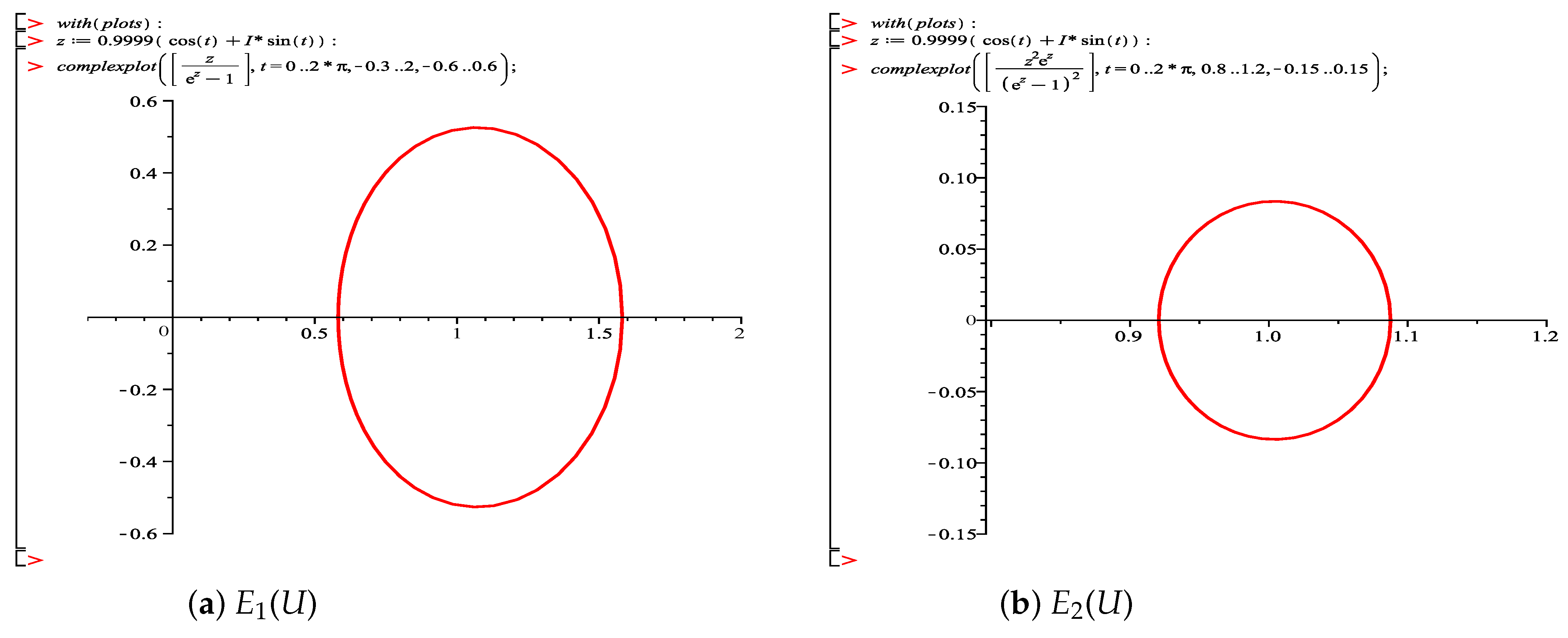
In mathematics, Einstein function is a name occasionally used for one of the functions (see [18,19]): .
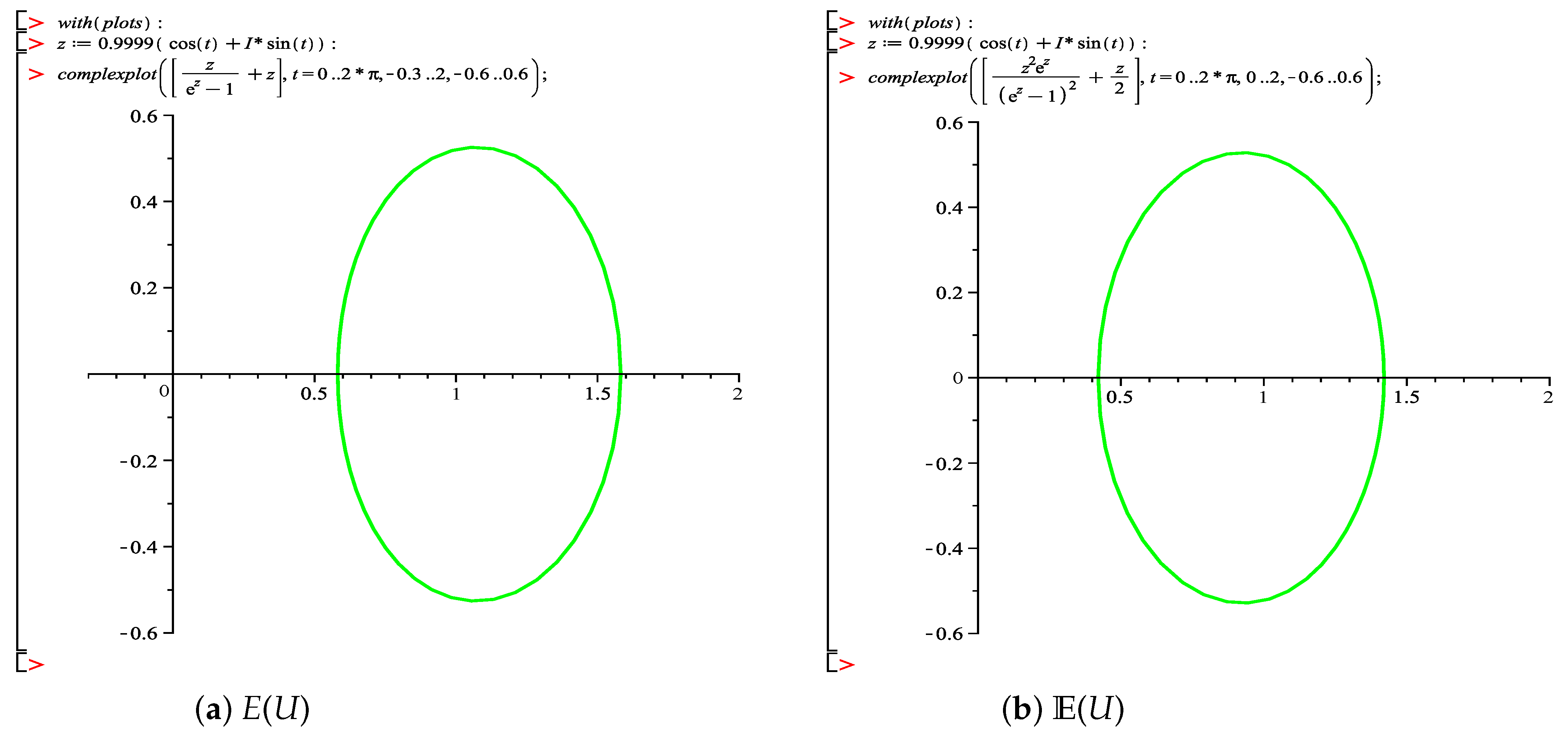
It is easily noticed that both and have these nice properties (see Figure 1); the image domain of ( are convex functions with ∀) is symmetric along the real axis and starlike about . Unfortunately, , thus, we shall define the new functions and . Now, we can say that (see Figure 2).
The series representations are given as follows:
and
where is the nth Bernoulli number; it is known that the Bernoulli numbers can be defined by the contour integral (see [20])
where the contour encloses the origin, has radius less than , and is traversed in a counterclockwise direction; the first few members are
and
Here, in this paper, we will deal with the first function E, the function is left as open problem.
Let be the subfamily of consisting of all functions of the form (1) which are univalent in U.
It is well known, by using the Koebe one-quarter theorem [21], that every univalent function containing a disc of radius has an inverse function , which is defined by
and
A function is said to be bi-univalent in U if both f and are univalent in U. Let denote the subfamily of , consisting of all bi-univalent functions defined on the unit disc U. Since has the Maclaurin series expansion given by (1), a simple calculation shows that its inverse has the series expansion
Examples of functions in the class are
and so on. However, the familiar Koebe function is not a member of . Other common examples of functions in , such as
are also not members of .
Now, we recall some notations about the q-difference operator which is used in investigating our main families. In view of Annaby and Mansour [22], the q-difference operator is defined by
and
We note that and .
Definition 1
The aim of this article is to introduce new subfamilies of analytic bi-univalent functions subordinate to the Einstein function . Furthermore, we deduce some estimations to , and also the Fekete–Szegö inequalities for the functions that belong to these subfamilies.
Definition 2.
Definition 3.
Lemma 2
Then,
2. Main Results
Unless otherwise mentioned, we assume in the reminder of this article that , , , , , and also .
Theorem 1.
Let , then
where
Proof.
Let f and g be in , then, it satisfies the conditions (7) and (8). However, according to subordination principle Definition 1 and Lemma 2, there exist two Schwarz functions and of the form
such that
and
After some simple calculations, we deduce
By substituting from (20), (21), (18) and (19) into (16) and (17), and by comparing the coefficients on both sides, we obtain
However, from Equation (22), we can deduce
Thus, by virtue of Lemma 2, we find
On the other hand, from the properties of the modulus, the term . Then, we conclude
Thus, the proof is completed. □
Theorem 2.
Let , then
where
Proof.
Suppose f and g are in , then they satisfy the conditions (7) and (8). According to subordination principle Definition 1 and Lemma 2, there exist two Schwarz functions of the form
such that
and
With some simple calculations, we get
and
By substituting from (18), (19), (40) and (41) into (38) and (39) as well as by comparing the coefficients on both sides, we conclude
and
On the other hand, from Equation (42), we can write
By the virtue of (51), we can get the desired result. Thus, we completed the proof. □
Theorem 3.
Proof.
Thus,
Now, applying Lemma 1 to (58), we can obtain the desired result directly. Thus, we completed the proof. □
Theorem 4.
Author Contributions
Formal analysis, A.H.E.-Q.; Methodology, M.A.M.; Resources, I.S.E. All authors have read and agreed to the published version of the manuscript.
Funding
The authors would like to thank the Common First Year Research Unit King Saud University for giving us the funds for this article.
Institutional Review Board Statement
Not applicable.
Informed Consent Statement
Not applicable.
Data Availability Statement
No data were used in this paper.
Conflicts of Interest
The authors declare no conflict of interest.
References
- Ma, W.C.; Minda, D. Unified treatment of some special classes of univalent functions. In Proceedings of the Conference on Complex Analysis; American Mathematical Society: Rhode Island, RI, USA, 1992; pp. 157–169. [Google Scholar]
- Janowski, W. Extremal problems for a family of functions with positive real part and for some related families. Ann. Pol. Math. 1971, 23, 159–177. [Google Scholar] [CrossRef] [Green Version]
- Ahmad, K.; Arif, M.; Liu, J.L. Convolution properties for a family of analytic functions involving q-analogue of Ruscheweyh differential operator. Turk. J. Math. 2019, 43, 1712–1720. [Google Scholar] [CrossRef] [Green Version]
- Arif, M.; Ahmad, K.; Liu, J.L.; Sokół, J. A new class of analytic functions associated with Sălăgean operator. J. Funct. Spaces 2019, 2019, 6157394. [Google Scholar] [CrossRef] [Green Version]
- Shi, L.; Khan, Q.; Srivastava, G.; Liu, J.L.; Arif, M. A study of multivalent q-starlike functions connected with circular domain. Mathematics 2019, 7, 670. [Google Scholar] [CrossRef] [Green Version]
- Srivastava, H.M.; Khan, B.; Khan, N.; Ahmad, Q.Z. Coeffcient inequalities for q-starlike functions associated with the Janowski functions. Hokkaido Math. J. 2019, 48, 407–425. [Google Scholar] [CrossRef]
- Srivastava, H.M.; Tahir, M.; Khan, B.; Ahmad, Q.Z.; Khan, N. Some general classes of q-starlike functions associated with the Janowski functions. Symmetry 2019, 11, 292. [Google Scholar] [CrossRef] [Green Version]
- Sokoł, J.; Stankiewicz, J. Radius of convexity of some subclasses of strongly starlike functions. Zesz. Nauk. Politech. Rzesz. Mat. 1996, 19, 101–105. [Google Scholar]
- Mendiratta, R.; Nagpal, S.; Ravichandran, V. On a subclass of strongly starlike functions associated with exponential function. Bull. Malays. Math. Sci. Soc. 2015, 38, 365–386. [Google Scholar] [CrossRef]
- Kumar, S.; Ravichandran, V. A subclass of starlike functions associated with a rational function. Southeast Asian Bull. Math. 2016, 40, 199–212. [Google Scholar]
- Cho, N.E.; Kumar, V.; Kumar, S.S.; Ravichandran, V. Radius problems for starlike functions associated with the sine function. Bull. Iran. Math. Soc. 2019, 45, 213–232. [Google Scholar] [CrossRef]
- Sharma, K.; Jain, N.K.; Ravichandran, V. Starlike functions associated with a cardioid. Afr. Mat. 2016, 27, 923–939. [Google Scholar] [CrossRef]
- Ravichandran, V.; Sharma, K. Sufficient conditions for starlikeness. J. Korean Math. Soc. 2015, 52, 727–749. [Google Scholar] [CrossRef] [Green Version]
- Sharma, K.; Ravichandran, V. Application of subordination theory to starlike functions. Bull. Iran. Math. Soc. 2016, 42, 761–777. [Google Scholar]
- Alotaibi, A.; Arif, M.; Alghamdi, M.A.; Hussain, S. Starlikness associated with cosine hyperbolic function. Mathematics 2020, 8, 1118. [Google Scholar] [CrossRef]
- Kargar, R.; Ebadian, A.; Sokół, J. On booth lemniscate and starlike functions. Anal. Math. Phys. 2019, 9, 1–12. [Google Scholar] [CrossRef]
- Raina, R.K.; Sokol, J. On coefficient estimates for a certain class of starlike functions. Hacet. J. Math. Stat. 2015, 44, 1427–1433. [Google Scholar] [CrossRef]
- Abramowitz, M.; Stegun, I.A. Debye Functions, §27.1. In Handbook of Mathematical Functions with Formulas, Graphs, and Mathematical Tables, 9th ed.; Dover: New York, NY, USA, 1972; pp. 999–1000. [Google Scholar]
- Lemmon, E.W.; Span, R. Short Fundamental Equations of State for 20 Industrial Fluids. J. Chem. Eng. Data 2006, 51, 785–850. [Google Scholar] [CrossRef]
- Arfken, G. Bernoulli Numbers, Euler-Maclaurin Formula, §5.9. In Mathematical Methods for Physicists, 3rd ed.; Academic Press: Orlando, FL, USA, 1985; pp. 327–338. [Google Scholar]
- Duren, P.L. Univalent Functions, Grundlehen der Mathematischen Wissenschaften 259; Springer: New York, NY, USA; Berlin/Heidelberg, Germany; Tokyo, Japan, 1983. [Google Scholar]
- Annaby, M.H.; Mansour, Z.S. Q-Fractional Calculus and Equations; Springer: New York, NY, USA, 2012; Volume 2056. [Google Scholar]
- Miller, S.S.; Mocanu, P.T. Differenatial Subordinations: Theory and Applications; Series on Monographs and Textbooks in Pure and Appl. Math. No. 255; Marcel Dekker, Inc.: New York, NY, USA, 2000. [Google Scholar]
- Bulboaca, T. Differential Subordinations and Superordinations: Recent Results; House of Science Book Publication: Cluj-Napoca, Romania, 2005. [Google Scholar]
- Zaprawa, P. Estimates of initial coefficients for bi-univalent functions. Abst. Appl. Anal. 2014, 2014, 357480. [Google Scholar] [CrossRef]
- El-Qadeem, A.H.; Mamon, M.A. Estimation of initial Maclaurin coefficients of certain subclasses of bounded bi-univalent functions. J. Egypt. Math. Soc. 2019, 27, 16. [Google Scholar] [CrossRef] [Green Version]
- Kanas, S.; Adegani, E.A.; Zireh, A. An unified approach to second Hankel determinant of bi-Subordinate functions. Mediterr. J. Math. 2017, 14, 233. [Google Scholar] [CrossRef]
Figure 1.
The images of unit disc U of the Einstein functions and .

Figure 2.
The images of unit disc U of the modified Einstein functions E and .

Publisher’s Note: MDPI stays neutral with regard to jurisdictional claims in published maps and institutional affiliations. |
© 2022 by the authors. Licensee MDPI, Basel, Switzerland. This article is an open access article distributed under the terms and conditions of the Creative Commons Attribution (CC BY) license (https://creativecommons.org/licenses/by/4.0/).
Share and Cite
MDPI and ACS Style
El-Qadeem, A.H.; Mamon, M.A.; Elshazly, I.S. Application of Einstein Function on Bi-Univalent Functions Defined on the Unit Disc. Symmetry 2022, 14, 758. https://doi.org/10.3390/sym14040758
AMA Style
El-Qadeem AH, Mamon MA, Elshazly IS. Application of Einstein Function on Bi-Univalent Functions Defined on the Unit Disc. Symmetry. 2022; 14(4):758. https://doi.org/10.3390/sym14040758
Chicago/Turabian StyleEl-Qadeem, Alaa H., Mohamed A. Mamon, and Ibrahim S. Elshazly. 2022. "Application of Einstein Function on Bi-Univalent Functions Defined on the Unit Disc" Symmetry 14, no. 4: 758. https://doi.org/10.3390/sym14040758
Note that from the first issue of 2016, this journal uses article numbers instead of page numbers. See further details here.