Lie Symmetries, Closed-Form Solutions, and Various Dynamical Profiles of Solitons for the Variable Coefficient (2+1)-Dimensional KP Equations

Abstract

This investigation focuses on two novel Kadomtsev–Petviashvili (KP) equations with time-dependent variable coefficients that describe the nonlinear wave propagation of small-amplitude surface waves in narrow channels or large straits with slowly varying width and depth and non-vanishing vorticity. These two variable coefficients, Kadomtsev–Petviashvili (VCKP) equations in (2+1)-dimensions, are the main extensions of the KP equation. Applying the Lie symmetry technique, we carry out infinitesimal generators, potential vector fields, and various similarity reductions of the considered VCKP equations. These VCKP equations are converted into nonlinear ODEs via two similarity reductions. The closed-form analytic solutions are achieved, including in the shape of distinct complex wave structures of solitons, dark and bright soliton shapes, double W-shaped soliton shapes, multi-peakon shapes, curved-shaped multi-wave solitons, and novel solitary wave solitons. All the obtained solutions are verified and validated by using back substitution to the original equation through Wolfram Mathematica. We analyze the dynamical behaviors of these obtained solutions with some three-dimensional graphics via numerical simulation. The obtained variable coefficient solutions are more relevant and useful for understanding the dynamical structures of nonlinear KP equations and shallow water wave models.

1. Introduction

A large number of physical problems, for example, in the branches of mathematical sciences, nonlinear dynamics, optical engineering, plasma physics, biology physics, fluid dynamics, nonlinear phenomena, and many others, are governed by nonlinear evolution equations (NLEEs). For this reason, the exact closed-form solutions of governed equations have great interest and pay much more attention in the research. These solutions are evaluated to understand the dynamical behavior of the concerned problem. Generally, there are no straightforward formulas for determining the closed-form solutions, even for simple NLPDEs in the view of linear theory. In literature, various effective transformation techniques are developed for obtaining exact solutions or explicit closed-form solutions of the NLEEs, for instance, Darboux transformation method [1], inverse scattering transform method [2], Hirota method [3], Linear superposition principle [4], simplest equation method [5], Bell polynomial approach [6], extended simplest equation method [7], F-expansion method [8], Bäcklund transformation [9], multiple exp-function methods [10], extended sinh-Gordon method [11], direct test functions method [12] and many other mathematical techniques.

The Norwegian Mathematician, Marius Sophus Lie, during the period 1872–1899, contributed to innovation in the province of general integration theory for ordinary differential equations and therefore stated as Lie’s theory. This is an effective and powerful tool for generating explicit closed-form solutions for NLEEs. The analytical closed-form solutions are constructed with the help of the group-theoretic method which may serve as a benchmark in the dynamics of multi-wave solitons, dynamical wave structure of solitons, and mechanism of different types of NLEEs [13]. The applications of the Lie symmetry method embrace different areas such as bifurcation theory, algebraic topology, fiber optics, differential geometry, plasma physics, hydrodynamics relativity, control theory, classical mechanics, numerical analysis, nonlinear dynamics, oceanography, plasma physics, and many others.

The KP equation, in standard form, is written as

$${(u_t+u{u}_x+u_{xxx})}_x+3u_{yy}=0.$$

(1)

The physical circumstances in which nonlinear equations arise tend to be idealized intensely due to the assumption of constant coefficients and inhomogeneities of media, and thus the study of nonlinear equations with variable coefficients has gained interest in order to obtain various soliton solutions. Our interest in this paper is to investigate the following equations which are obtained by introducing two novel variable-coefficient extensions of the KP equation [14] described as

$$\begin{array}{cc}\hfill & {(u_t+u{u}_x+u_{xxx})}_x+3u_{yy}+g\left(t\right)u_{xy}=0,\hfill \end{array}$$

(2)

and

$$\begin{array}{c}\hfill {(u_t+u{u}_x+u_{xxx})}_x+3u_{yy}+h\left(t\right)u_{xx}=0,\end{array}$$

(3)

where $u(x,y,t)$ is the wave amplitude with two scaled spatial variables and temporal variable $x,y$ and t respectively, and $g\left(t\right)$ and $h\left(t\right)$ are the functional parameters of variable t. These two KP Equations (2) and (3) describe the wave-propagation of small-amplitude surface waves in narrow channels or large straits of slowly changing width and depth and non-vanishing vorticity. A series of equations can be enlisted by considering different forms for the functional parameters $g\left(t\right)$ and $h\left(t\right)$, that proved to be integrable (See Wazwaz [14]). In Equations (2) and (3), these time-dependent variable coefficients $g\left(t\right)$ and $h\left(t\right)$ are resulting from the physical and geometrical inhomogeneities, like material density, variation in radius, and many others [15]. For considering $g\left(t\right)$ and $h\left(t\right)$ equal to zero, Equations (2) and (3) will be converted to the original KP equation. The KP equations with variable-coefficients have been studied extensively by many mathematicians in the literature [14,15,16,17,18,19,20,21]. Recently, Wazwaz [14] studied these new two KP equations with variable coefficients and obtained several complex soliton solutions and multiple solitons using the simplified Hirota’s method.

The prime objective of this article is to introduce the Lie symmetry analysis for obtaining exact closed-form solutions to the (2+1)-dimensional VCKP equations which describe the wave-amplitude of the shallow-water waves in fluid dynamics or ion-acoustic solitary waves in dusty plasmas. Based on the Lie symmetry technique, we accomplished exact solutions and dynamics of complexion profiles of the obtained soliton solutions of two novel Kadomtsev–Petviashvili (KP) Equations (2) and (3). The numerous explicit closed-form solutions are produced in the form of distinct complex dynamics of soliton shapes such as, dark and bright soliton shape, double W-shaped soliton shape, curved-shaped multiple soliton shape, double W-shaped soliton shape, and novel solitary wave solitons. All the findings have been verified with computerized symbolic computation via Wolfram Mathematica. The exact solutions generated are completely novel and have never been reported in the literature. One may refer to [13,22,23,24,25] to explore more about the Lie symmetry analysis method for various NLEEs.

The rest of the article is summarized as follows: Section 2 deals with the brief explanation of Lie symmetry analysis for first and second variable coefficients of KP equations. Section 3 derives various similarity reductions and numerous exact invariant solutions for the first VCKP equation and second VCKP equation. We also analyze the dynamical behaviors of some obtained solutions through three-dimensional graphics based on numerical simulations. In Section 4, the physical explanations of the newly established solutions are discussed. Then, the article ends with the conclusion described in Section 5.

2. Lie Symmetries

The Lie symmetry technique is a highly powerful, robust and proficient mathematical tool to solve nonlinear PDEs. This technique has been fruitfully and constructively utilized in solving numerous nonlinear complex physical models [13,22]. In the present section, we aim to discuss the Lie symmetry method (LSM) to generate the infinitesimals generators and exact invariant solutions of the first and second variable coefficient KP Equation (3). Considering an one-parameter group of infinitesimals transformations:

$$\begin{array}{cc}\hfill x^{*}& =x+ϵ\xi +O\left({ϵ}^2\right),\hfill \\ \hfill y^{*}& =y+ϵ\varphi +O\left({ϵ}^2\right),\hfill \\ \hfill t^{*}& =t+ϵ\tau +O\left({ϵ}^2\right),\hfill \\ \hfill u^{*}& =u+ϵ\eta +O\left({ϵ}^2\right),\hfill \end{array}$$

(4)

where $ϵ$ is a small Lie group parameter and $\xi ,\varphi ,\tau ,$ and $\eta$ are the infinitesimals generators of $(x,y,t,u)$. Therefore, the associated vector field is

$$\begin{array}{c}\hfill \mathfrak{T}=\xi {\partial }_x+\varphi {\partial }_y+\tau {\partial }_t+\eta {\partial }_u.\end{array}$$

(5)

Eventually, the fourth-prolongation $P{r}^4$ of the vector field $\mathfrak{T}$ is acquired as

$$\begin{array}{c}\hfill P{r}^4\mathfrak{T}=\mathfrak{T}+{\eta }^x\frac{\partial }{\partial u_x}+{\eta }^y\frac{\partial }{\partial u_y}+{\eta }^{xx}\frac{\partial }{\partial u_{xx}}+{\eta }^{xy}\frac{\partial }{\partial u_{xy}}+{\eta }^{yt}\frac{\partial }{\partial u_{yt}}+\cdots .\end{array}$$

(6)

Applying the above prolongation including invariant condition $P{r}^{\left(4\right)}\mathfrak{T}(\Delta )=0,$ whenever $\Delta =0$ to the first VCKP Equation (2) and second VCKP Equation (3), we conclude that

$$\begin{array}{cc}\hfill & {\eta }^{xxxx}+u{\eta }^{xx}+h\left(t\right){\eta }^{xx}+{\eta }^{tx}+3{\eta }^{yy}+2{\eta }^x{u}_x=0,\hfill \end{array}$$

(7)

$$\begin{array}{cc}\hfill & {\eta }^{xxxx}+u{\eta }^{xx}+g\left(t\right){\eta }^{xy}+{\eta }^{tx}+3{\eta }^{yy}+2{\eta }^x{u}_x=0,\hfill \end{array}$$

(8)

where

$$\begin{array}{cc}\hfill {\eta }^x& =D_x\eta -u_x{D}_x\xi -u_y{D}_x\varphi -u_t{D}_x\tau ,\hfill \\ \hfill {\eta }^y& =D_y\eta -u_x{D}_y\xi -u_y{D}_y\varphi -u_t{D}_y\tau ,\hfill \\ \hfill {\eta }^{xx}& =D_x{\eta }^x-u_{xx}{D}_x\xi -u_{xy}{D}_x\varphi -u_{xt}{D}_x\tau ,\hfill \\ \hfill {\eta }^{yy}& =D_y{\eta }^y-u_{xy}{D}_y\xi -u_{yy}{D}_y\varphi -u_{yt}{D}_y\tau ,\hfill \\ \hfill {\eta }^{xt}& =D_t{\eta }^x-u_{xx}{D}_t\xi -u_{xy}{D}_t\varphi -u_{xt}{D}_t\tau ,\hfill \\ \hfill {\eta }^{xxxx}& =D_x{\eta }^{xxx}-u_{xxxx}{D}_x\xi -u_{xxxy}{D}_x\varphi -u_{xxxt}{D}_x\tau ,\hfill \end{array}$$

(9)

and the operators $D_x,D_y$, and $D_t$ are total derivatives with regard to $x,y$, and t, respectively. On solving invariance condition, we substitute all the above expressions from Equation (9) into Equations (7) and (8) and consequently, we acquire the following set of determining equations

$$\begin{array}{cc}\hfill & {\left(\tau \right)}_u=0,{\left(\tau \right)}_x=0,{\left(\tau \right)}_y=0,{\left(\xi \right)}_u=0,{\left(\xi \right)}_x=\frac{1}{3}{\left(\tau \right)}_t,{\left(\xi \right)}_y=\frac{1}{18}{\left(\tau \right)}_{t}g\left(t\right)+\frac{1}{6}\tau g^{\prime }\left(t\right)-\frac{1}{6}{\left(\varphi \right)}_t,\hfill \\ \hfill & {\left(\varphi \right)}_u=0,{\left(\varphi \right)}_x=0,{\left(\varphi \right)}_y=\frac{2}{3}{\left(\tau \right)}_t,\left(\eta \right)=\frac{1}{18}(-12u+g^2\left(t\right)){\left(\tau \right)}_t+\frac{1}{6}\tau g\left(t\right)g^{\prime }\left(t\right)-\frac{1}{6}{\left(\varphi \right)}_t+{\left(\xi \right)}_t,\hfill \end{array}$$

(10)

and

$$\begin{array}{cc}\hfill & {\left(\tau \right)}_u=0,{\left(\tau \right)}_x=0,{\left(\tau \right)}_y=0,{\left(\tau \right)}_t=\frac{3}{2}{\left(\varphi \right)}_y,{\left(\xi \right)}_u=0,{\left(\xi \right)}_x=\frac{1}{2}{\left(\varphi \right)}_y,\hfill \\ \hfill & {\left(\xi \right)}_y=-\frac{1}{6}{\left(\varphi \right)}_t,{\left(\varphi \right)}_u=0,{\left(\varphi \right)}_x=0,{\left(\varphi \right)}_{yy}=0,\left(\eta \right)=(-u-h\left(t\right)){\left(\varphi \right)}_y-\tau h^{\prime }\left(t\right)+{\left(\xi \right)}_t,\hfill \end{array}$$

(11)

respectively.

2.1. Lie Symmetry Analysis for First VCKP Equation

We attain the desired infinitesimal generators of the first VCKP Equation (2) after solving the system of determining Equation (10)

$$\begin{array}{cc}\hfill & \xi =\frac{1}{3}{f}_1^{\prime }\left(t\right)x-\frac{1}{18}{f}_1^{″}\left(t\right)y^2+\frac{1}{18}{f}_1^{\prime }\left(t\right)yg\left(t\right)+\frac{1}{6}{f}_1\left(t\right)y{g}^{\prime }\left(t\right)-\frac{1}{6}{f}_2^{\prime }\left(t\right)y+f_3\left(t\right),\hfill \\ \hfill & \varphi =\frac{2}{3}{f}_1^{\prime }\left(t\right)y+f_2\left(t\right),\tau =f_1\left(t\right),\hfill \\ \hfill & \eta =\frac{1}{18}(-yg\left(t\right)+6x)f_1^{″}\left(t\right)-\frac{1}{18}{y}^2{f}_1^{‴}\left(t\right)-\frac{1}{6}{f}_2^{″}\left(t\right)y+\frac{1}{6}y{f}_1\left(t\right)g^{″}\left(t\right)+\frac{1}{18}(4y{g}^{\prime }\left(t\right)\hfill \\ \hfill & +g^2\left(t\right)-12u)f_1^{\prime }\left(t\right)+\frac{1}{6}g\left(t\right)f_1\left(t\right)g^{\prime }\left(t\right)-\frac{1}{6}{f}_2^{\prime }\left(t\right)g\left(t\right)+f_3^{\prime }\left(t\right),\hfill \end{array}$$

(12)

where $f_1\left(t\right),f_2\left(t\right)\mathrm{and}{f}_3\left(t\right)$ are arbitrary functional parameters of t. Now, we take $f_1\left(t\right)=c_{1}t+c_2$ and $f_2\left(t\right)=c_{3}t+c_4$, where $c_1,c_2,c_3$ and $c_4$ are any four arbitrary constants.

Using the Equation (12), therefore we construct the following vector fields of the first VCKP Equation (2)

$$\begin{array}{cc}\hfill & {\mathfrak{T}}_1=\frac{2}{3}y\frac{\partial }{\partial y}+t\frac{\partial }{\partial t}+\left(\frac{1}{6}yt{g}^{″}\left(t\right)+\frac{1}{18}(4y{g}^{\prime }\left(t\right)+g^2\left(t\right)-12u)+\frac{1}{6}tg\left(t\right)g^{\prime }\left(t\right)\right)\frac{\partial }{\partial u},\hfill \\ \hfill & +\left(\frac{1}{18}(yg\left(t\right)+6x)+\frac{1}{6}yt{g}^{\prime }\left(t\right)\right)\frac{\partial }{\partial x},\hfill \\ \hfill & {\mathfrak{T}}_2=\frac{1}{6}y{g}^{\prime }\left(t\right)\frac{\partial }{\partial x}+\frac{\partial }{\partial t}+\frac{1}{6}(y{g}^{″}\left(t\right)+g\left(t\right)g^{\prime }\left(t\right))\frac{\partial }{\partial u},\hfill \\ \hfill & {\mathfrak{T}}_3=-\frac{1}{6}y\frac{\partial }{\partial x}+t\frac{\partial }{\partial y}-\frac{1}{6}g\left(t\right)\frac{\partial }{\partial u},{\mathfrak{T}}_4=\frac{\partial }{\partial y},{\mathfrak{T}}_5\left(f_3\right)=f_3\left(t\right)\frac{\partial }{\partial x}+f_3^{\prime }\left(t\right)\frac{\partial }{\partial u}.\hfill \end{array}$$

(13)

2.2. Lie Symmetry Analysis for Second Variable Coefficient KP Equation

We receive the desired infinitesimal generators of the second VCKP Equation (3) after solving the system of determining Equation (11)

$$\begin{array}{cc}\hfill & \xi =\frac{1}{2}{f}_1^{\prime }\left(t\right)x-\frac{1}{12}{f}_1^{″}\left(t\right)y^2-\frac{1}{6}{f}_2^{\prime }\left(t\right)y+f_3\left(t\right),\varphi =f_1^{\prime }\left(t\right)y+f_2\left(t\right),\tau =\frac{3}{2}{f}_1\left(t\right)+c_1,\hfill \\ \hfill & \eta =-h\left(t\right)f_1^{\prime }\left(t\right)-(\frac{3}{2}{f}_1\left(t\right)+c_1)h^{\prime }\left(t\right)-f_1^{\prime }\left(t\right)u+\frac{1}{2}{f}_1^{″}\left(t\right)x-\frac{1}{12}{y}^2{f}_1^{‴}\left(t\right)-\frac{1}{6}{f}_2^{″}\left(t\right)y+f_3^{\prime }\left(t\right),\hfill \end{array}$$

(14)

where $f_1\left(t\right),f_2\left(t\right)$ and $f_3\left(t\right)$ are any four arbitrary function parameters of t. We take $f_1\left(t\right)=c_{5}t+c_6$, where $c_5$ and $c_6$ are arbitrary constants.

With the help of Equation (14), therefore we construct the following vector fields of the first VCKP Equation (3)

$$\begin{array}{cc}\hfill & {\mathfrak{F}}_1=\frac{\partial }{\partial t}-h^{\prime }\left(t\right)\frac{\partial }{\partial u},{\mathfrak{F}}_2=\frac{1}{2}x\frac{\partial }{\partial x}+y\frac{\partial }{\partial y}+\frac{3}{2}t\frac{\partial }{\partial t}+(-h\left(t\right)-\frac{3}{2}t{h}^{\prime }\left(t\right)-u)\frac{\partial }{\partial u},\hfill \\ \hfill & {\mathfrak{F}}_3\left(f_2\right)=-\frac{1}{6}{f}_2^{\prime }\left(t\right)y\frac{\partial }{\partial x}+f_2\left(t\right)\frac{\partial }{\partial y}-\frac{1}{6}y{f}_2^{″}\left(t\right)\frac{\partial }{\partial u},{\mathfrak{F}}_4\left(f_3\right)=f_3\left(t\right)\frac{\partial }{\partial x}+f_3^{\prime }\left(t\right)\frac{\partial }{\partial u}.\hfill \end{array}$$

(15)

3. Exact Invariant Solutions

This section applies the Lie symmetry technique to construct some new exact invariant solutions and exhibit some dynamics of complexiton solutions to the two novel variable coefficient KP equations.

3.1. Exact Solutions to the First VCKP Equation

First, we will study the useful linear combinations of vector fields for the first VCKP Equation (2) as

(i) ${\mathfrak{T}}_1$, (ii) ${\mathfrak{T}}_2$, (iii) ${\mathfrak{T}}_3$, (iv) ${\mathfrak{T}}_4$, (v) ${\mathfrak{T}}_5$, (vi) ${\mathfrak{T}}_4+{\mathfrak{T}}_5$.

The related Characteristic-Lagrange’s equation is

$$\begin{array}{c}\hfill \frac{dx}{\xi }=\frac{dy}{\varphi }=\frac{dt}{\tau }=\frac{du}{\eta }.\end{array}$$

Now, it is time to discuss these vector fields one after another via symbolic computations.

3.1.1. Vector Field ${\mathfrak{T}}_1$

The Lie symmetry ${\mathfrak{T}}_1$ forms

$$\begin{array}{c}\hfill u(x,y,t)=\frac{1}{t^{2/3}}U(X,Y)+\frac{1}{6}(t^{2/3}Y{g}^{\prime }\left(t\right)+g{\left(t\right)}^2),\end{array}$$

(16)

where $U(X,Y)$ is any arbitrary function of $X=\frac{x}{\sqrt[3]{t}}-\frac{1}{6}\sqrt[3]{t}Yg\left(t\right)$ and $Y=\frac{y}{t^{2/3}}$. Combining (16) into (2), we will arrives

$$\begin{array}{c}\hfill 54U_{YY}+18U_X^2+18U{U}_{XX}+18U_{XXXX}-6X{U}_{XX}-18U_X-12Y{U}_{XY}=0.\end{array}$$

(17)

Apply the LSM on Equation (17), then new infinitesimals are given as:

$$\begin{array}{cc}& {\xi }_X=\frac{1}{36}{b}_1(-3Y^2+18X)-\frac{1}{9}{b}_{2}Y+b_3,{\xi }_Y=Y{b}_1+b_2,\hfill \\ \hfill & {\eta }_U=\frac{1}{108}{b}_1(9Y^2-108U+54X)+\frac{1}{27}{b}_{2}Y+\frac{1}{3}{b}_3,\hfill \end{array}$$

(18)

where $b_i$’s $(1\le i\le 3)$ are arbitrary constants.

Case: $b_1=0$ yields

$$\begin{array}{c}\hfill \frac{dX}{-\frac{1}{9}{b}_{2}Y+b_3}=\frac{dY}{b_2}=\frac{dU}{\frac{1}{27}{b}_{2}Y+\frac{1}{3}{b}_3}.\end{array}$$

(19)

Thus, similarity transformation construct the following form

$$\begin{array}{c}\hfill U(X,Y)=\frac{1}{27}\left(9B_{3}Y+\frac{Y^2}{2}\right)+H\left(\mathrm{W}\right)\mathrm{where}\mathrm{W}=-B_{3}Y+X+\frac{Y^2}{18}.\end{array}$$

(20)

Taking this value of U in (17) produces the nonlinear fourth-order ODEs

$$\begin{array}{c}\hfill \left(54B_3^2+18H-6\mathrm{W}\right)H^{″}+18H^{\left(4\right)}+18{\left(H^{\prime }\right)}^2-12H^{\prime }+2=0.\end{array}$$

(21)

Primitives of (21) are

$$\begin{array}{c}\hfill H\left(\mathrm{W}\right)=-3B_3^2-\frac{12}{{\mathrm{W}}^2}+\frac{\mathrm{W}}{3}\mathrm{and}H\left(\mathrm{W}\right)={\mathcal{Q}}_1+\frac{\mathrm{W}}{3},\end{array}$$

(22)

where ${\mathcal{Q}}_1$ is arbitrary constant. Comprising Equations (16), (20) and (22), we acquire explicit solutions of the first VCKP (2)

$$\begin{array}{cc}\hfill & u(x,y,t)=\frac{x}{3t}+\frac{y^2}{27t^2}-\frac{3888t^2}{\left(-18B_3{t}^{2/3}y-3tyg\left(t\right)+18tx+y^2\right){}^2}-\frac{3B_3^2}{t^{2/3}}\hfill \\ \hfill & +\frac{1}{6}y{g}^{\prime }\left(t\right)-\frac{yg\left(t\right)}{18t}+\frac{g{\left(t\right)}^2}{12},\hfill \end{array}$$

(23)

$$\begin{array}{cc}\hfill & u(x,y,t)=\frac{\left(6ty{g}^{\prime }\left(t\right)-2yg\left(t\right)+3tg{\left(t\right)}^2+36{\mathcal{Q}}_1\sqrt[3]{t}\right)}{36t}+\frac{\left(9tx+y^2\right)}{27t^2}.\hfill \end{array}$$

(24)

3.1.2. Vector Field ${\mathfrak{T}}_2$

The Lie symmetry ${\mathfrak{T}}_1$ forms

$$\begin{array}{c}\hfill u(x,y,t)=U(X,Y)+\frac{1}{6}Y{g}^{\prime }\left(t\right)+\frac{g{\left(t\right)}^2}{12},\end{array}$$

(25)

where U is any arbitrary function of $X=x-\frac{1}{6}Yg\left(t\right)$ and $Y=y$. Combining (25) into (2) gives

$$\begin{array}{c}\hfill 3U_{YY}+U{U}_{XX}+U_X^2+U_{XXXX}=0.\end{array}$$

(26)

Again, we use the LSM on Equation (26), thus new infinitesimals are given as:

$$\begin{array}{cc}& {\xi }_X=\frac{1}{2}{b}_{1}X+b_3,{\xi }_Y=Y{b}_1+b_2,{\eta }_U=-b_{1}U,\hfill \end{array}$$

(27)

where $b_i$’s $(1\le i\le 3)$ are arbitrary constant parameters.

Characterstic equation for Equation (27) is given by

$$\begin{array}{c}\hfill \frac{dX}{\frac{1}{2}{b}_{1}X+b_3}=\frac{dY}{Y{b}_1+b_2}=\frac{dU}{-b_{1}U},\end{array}$$

(28)

then, we have

$$\begin{array}{c}\hfill U(X,Y)=\frac{H\left(\mathrm{W}\right)}{b_{1}Y+b_2}\mathrm{with}\mathrm{W}=\frac{1}{\sqrt{b_{1}Y+b_2}}\left(\frac{2b_3}{b_1}+X\right).\end{array}$$

(29)

Taking this value of U in (26), then Equation (26) transformed into ODEs

$$\begin{array}{c}\hfill \left(4H+3b_1^2{\mathrm{W}}^2\right)H^{″}+4H^{\left(4\right)}+4{\left(H^{\prime }\right)}^2+24b_1^{2}H+21b_1^2\mathrm{W}{H}^{\prime }=0.\end{array}$$

(30)

The solutions of Equation (30) are

$$\begin{array}{c}\hfill H\left(\mathrm{W}\right)=-3b_1^2{\mathrm{W}}^2-\frac{12}{{\mathrm{W}}^2}\mathrm{and}H\left(\mathrm{W}\right)={\mathcal{Q}}_2-3b_1^2{\mathrm{W}}^2.\end{array}$$

(31)

where ${\mathcal{Q}}_2$ is arbitrary constant. Consequently, we arrive closed-form solutions of the first VCKP (2)

$$\begin{array}{cc}\hfill u(x,y,t)& =-\frac{\left(b_1(6x-yg\left(t\right))+12b_3\right){}^2}{12{\left(b_{1}y+b_2\right)}^2}-\frac{12}{\left(\frac{2b_3}{b_1}-\frac{1}{6}yg\left(t\right)+x\right){}^2}+\frac{1}{6}y{g}^{\prime }\left(t\right)+\frac{g{\left(t\right)}^2}{12},\hfill \end{array}$$

(32)

$$\begin{array}{cc}\hfill u(x,y,t)& =\frac{{\mathcal{Q}}_2}{b_{1}y+b_2}-\frac{\left(b_1(6x-yg\left(t\right))+12b_3\right){}^2}{12{\left(b_{1}y+b_2\right)}^2}+\frac{1}{6}y{g}^{\prime }\left(t\right)+\frac{g{\left(t\right)}^2}{12}.\hfill \end{array}$$

(33)

3.1.3. Vector Field ${\mathfrak{T}}_3$

The Vector field ${\mathfrak{T}}_3$ establishes the similarity-form

$$\begin{array}{c}\hfill u(x,y,t)=U(X,T)-\frac{yg\left(T\right)}{6T},\end{array}$$

(34)

where U is any arbitrary function of $X=\frac{y^2}{12T}+x$ and $T=t$. Combining (34) into (2) which leads to the reduced equation

$$\begin{array}{c}\hfill \frac{U_X}{2T}+U_{XT}+U{U}_{XX}+U_X^2+U_{XXXX}=0.\end{array}$$

(35)

After utilizing the LSM on (35), we have the following new infinitesimals

$$\begin{array}{cc}\hfill {\xi }_X& =\frac{1}{2}X{b}_1\sqrt{T}+\frac{1}{3}X{b}_2+F_1\left(T\right),{\xi }_T=b_1{T}^{\frac{3}{2}}+b_{2}T,\hfill \\ \hfill {\eta }_U& =-\frac{2}{3}{b}_{2}U+\frac{1}{4}{b}_1\frac{X}{\sqrt{T}}+F_1^{\prime }\left(T\right)-U{b}_1\sqrt{T},\hfill \end{array}$$

(36)

where $b_i$’s $(1\le i\le 3)$ are arbitrary constants.

Case: $b_1=0$ and all other constants are non-zero

$$\begin{array}{c}\hfill \frac{dX}{\frac{1}{3}X{b}_2+F_1\left(T\right)}=\frac{dY}{b_{2}T}=\frac{dU}{-\frac{2}{3}{b}_{2}U+F_1^{\prime }\left(T\right)},\end{array}$$

(37)

which produces

$$\begin{array}{c}\hfill U(X,T)=\frac{1}{T^{2/3}}\left(\int \frac{F_1^{\prime }\left(T\right)}{b_2\sqrt[3]{T}}dT+H\left(\mathrm{W}\right)\right)\mathrm{with}\mathrm{W}=\frac{X}{\sqrt[3]{T}}-\int \frac{F_1\left(T\right)}{b_2{T}^{4/3}}dT.\end{array}$$

(38)

Substituting the value of $U(X,T)$ into (35), we get the fourth-order NLODEs

$$\begin{array}{c}\hfill 6H^{\left(4\right)}-2\mathrm{W}{H}^{″}+6H{H}^{″}+6{\left(H^{\prime }\right)}^2-3H^{\prime }=0.\end{array}$$

(39)

Primitives of (39) are

$$\begin{array}{c}\hfill H\left(\mathrm{W}\right)=\frac{\mathrm{W}}{2}-\frac{12}{{\mathrm{W}}^2}\mathrm{and}H\left(\mathrm{W}\right)={\mathcal{Q}}_3+\frac{\mathrm{W}}{2},\end{array}$$

(40)

where ${\mathcal{Q}}_3$ is arbitrary constant. As a result, we obtained explicit solutions to the first VCKP (2)

$$\begin{array}{cc}\hfill u(x,y,t)& =\frac{1}{2b_2{t}^{\frac{2}{3}}}\left(-\frac{3456b_2^3{t}^{8/3}}{\left(b_2\left(12tx+y^2\right)-12t^{4/3}\int \frac{F_1\left(t\right)}{t^{4/3}}dt\right){}^2}-\int \frac{F_1\left(t\right)}{t^{4/3}}dt+2\int \frac{F_1^{\prime }\left(t\right)}{\sqrt[3]{t}}dt\right)\hfill \\ \hfill & +\frac{x}{2t}+\frac{y^2}{24t^2}-\frac{yg\left(t\right)}{6t},\hfill \end{array}$$

(41)

$$\begin{array}{cc}\hfill u(x,y,t)& =\frac{1}{24b_2{t}^2}\left(b_2\left(-4tyg\left(t\right)+24{\mathcal{Q}}_3{t}^{4/3}+12tx+y^2\right)+24t^{4/3}\left(\int \frac{F_1^{\prime }\left(t\right)}{\sqrt[3]{t}}dt\right)\right)\hfill \\ & -\frac{1}{2b_2{t}^{\frac{2}{3}}}\left(\int \frac{F_1\left(t\right)}{t^{4/3}}dt\right).\hfill \end{array}$$

(42)

3.1.4. Vector Field ${\mathfrak{T}}_4$

The Lie symmetry ${\mathfrak{T}}_4$ establishes the similarity-form

$$\begin{array}{c}\hfill u(x,y,t)=U(X,T),\end{array}$$

(43)

where U is any arbitrary function with $X=x$ and $T=t$. Combining (43) into (2) which leads to the PDEs

$$\begin{array}{c}\hfill U_{XT}+U_X^2+U{U}_{XX}+U_{XXXX}=0.\end{array}$$

(44)

Utilizing of LSM on Equation (44) gives the following new infinitesimal generators

$$\begin{array}{c}\hfill {\xi }_X=\frac{1}{3}{b}_{1}X+F_1\left(T\right),{\xi }_T=T{b}_1+b_2,{\eta }_U=-\frac{2}{3}{b}_{1}U+F_1^{\prime }\left(T\right),\end{array}$$

(45)

where $b_i$’s $(1\le i\le 2)$ are arbitrary constants.

Case: Let us take $b_1=0$ and $b_2$ be non-zero.

Therefore, we have

$$\begin{array}{c}\hfill \frac{dX}{F_1\left(T\right)}=\frac{dT}{b_2}=\frac{dU}{F_1^{\prime }\left(T\right)},\end{array}$$

(46)

which yields

$$\begin{array}{c}\hfill U(X,T)=\frac{F_1\left(T\right)}{b_2}+H\left(\mathrm{W}\right)\mathrm{with}\mathrm{W}=X-\int \frac{F_1\left(T\right)}{b_2}dT.\end{array}$$

(47)

Using (44) and (47), we get an ODE

$$\begin{array}{c}\hfill H^{\left(4\right)}\left(\mathrm{W}\right)+H\left(\mathrm{W}\right)H^{″}\left(\mathrm{W}\right)+H^{\prime }{\left(\mathrm{W}\right)}^2=0.\end{array}$$

(48)

Primitive of (48), we arrive

$$\begin{array}{c}\hfill H\left(\mathrm{W}\right)=-\frac{12}{{\mathrm{W}}^2}.\end{array}$$

(49)

Accordingly, we acquire the soliton solution of the first VCKP (2):

$$\begin{array}{c}\hfill u(x,y,t)=\frac{F_1\left(t\right)}{b_2}-\frac{12}{{\left(x-\frac{\int F_1\left(t\right)dt}{b_2}\right)}^2}.\end{array}$$

(50)

3.1.5. Vector Field ${\mathfrak{T}}_5$

The Lie symmetry ${\mathfrak{T}}_5$ establishes the similarity-form

$$\begin{array}{c}\hfill u(x,y,t)=U(Y,T)+\frac{x{f}_3^{\prime }\left(t\right)}{f_3\left(t\right)},\end{array}$$

(51)

where $U(Y,T)$ any arbitrary function of $Y=y$ and $T=t$. Combining (51) into the Equation (2) which produce nonlinear PDE

$$\begin{array}{c}\hfill 3U_{YY}+\frac{f_3^{″}\left(T\right)}{f_3\left(T\right)}=0.\end{array}$$

(52)

On twice integration, we obtain

$$\begin{array}{c}\hfill U(Y,T)=Y{\mathcal{G}}_2\left(T\right)+{\mathcal{G}}_1\left(T\right)-\frac{Y^2{f}_3^{″}\left(T\right)}{6f_3\left(T\right)},\end{array}$$

(53)

where ${\mathcal{G}}_1\left(T\right)$ and ${\mathcal{G}}_2\left(T\right)$ are any two arbitrary functions of T.

Comprising (51) and (53), we arrive soliton-solution of the first VCKP (2)

$$\begin{array}{cc}\hfill u(x,y,t)& =\frac{6x{f}_3^{\prime }\left(t\right)-y^2{f}_3^{″}\left(t\right)}{6f_3\left(t\right)}+y{\mathcal{G}}_2\left(t\right)+{\mathcal{G}}_1\left(t\right).\hfill \end{array}$$

(54)

3.1.6. Vector Field ${\mathfrak{T}}_2+{\mathfrak{T}}_5$

For simplification, we take $f_3\left(t\right)=\frac{1}{6}{a}_0{g}^{\prime }\left(t\right)$

The Lie symmetry ${\mathfrak{T}}_2+{\mathfrak{T}}_5$ establishes the similarity expression

$$\begin{array}{c}\hfill u(x,y,t)=U(X,Y)+\frac{1}{6}{a}_0{g}^{\prime }\left(t\right)+\frac{1}{6}Y{g}^{\prime }\left(t\right)+\frac{g{\left(t\right)}^2}{12},\end{array}$$

(55)

where U is any arbitrary function of $X=-\frac{1}{6}{a}_{0}g\left(t\right)-\frac{1}{6}Yg\left(t\right)+x$ and $Y=y$. Combining (55) into (2), therefore the reduced PDE

$$\begin{array}{c}\hfill 3U_{YY}+U{U}_{XX}+U_X^2+U_{XXXX}=0.\end{array}$$

(56)

Again using LSM on (56), thus we obtain

$$\begin{array}{c}\hfill {\xi }_X=\frac{1}{2}{b}_{1}X+b_3,{\xi }_Y=Y{b}_1+b_2,{\eta }_U=-b_{1}U,\end{array}$$

(57)

where $b_i$’s $(1\le i\le 3)$ are arbitrary constant parameters.

From Equation (57), we arrive

$$\begin{array}{c}\hfill \frac{dX}{\frac{1}{2}{b}_{1}X+b_3}=\frac{dY}{Y{b}_1+b_2}=\frac{dU}{-b_{1}U},\end{array}$$

(58)

which provides

$$\begin{array}{c}\hfill U(X,Y)=\frac{H\left(\mathrm{W}\right)}{b_{1}Y+b_2}\mathrm{with}\mathrm{W}=\frac{1}{\sqrt{b_{1}Y+b_2}}\left(\frac{2b_3}{b_1}+X\right).\end{array}$$

(59)

Combining (56) and (59), then (56) transformed into a fourth-order nonlinear ODEs

$$\begin{array}{c}\hfill \left(4H+3b_1^2{\mathrm{W}}^2\right)H^{″}+4H^{\left(4\right)}+4{\left(H^{\prime }\right)}^2+24b_1^{2}H+21b_1^2\mathrm{W}{H}^{\prime }=0.\end{array}$$

(60)

Primitives of (60) are

$$\begin{array}{c}\hfill H\left(\mathrm{W}\right)=-3b_1^2{\mathrm{W}}^2-\frac{12}{{\mathrm{W}}^2}\mathrm{and}H\left(\mathrm{W}\right)={\mathcal{Q}}_4-3b_1^2{\mathrm{W}}^2,\end{array}$$

(61)

where ${\mathcal{Q}}_4$ is arbitrary constant. Combining Equations (55), (59) and (61), we arrive at the following closed-form solutions to the first VCKP (2)

$$\begin{array}{cc}\hfill u(x,y,t)& =\frac{1}{6}a{g}^{\prime }\left(t\right)-\frac{12}{{\left(-\frac{1}{6}(a+y)g\left(t\right)+\frac{2b_3}{b_1}+x\right)}^2}-\frac{{\left(b_1((a+y)g\left(t\right)-6x)-12b_3\right)}^2}{12{\left(b_{1}y+b_2\right)}^2}\hfill \\ \hfill & +\frac{1}{6}y{g}^{\prime }\left(t\right)+\frac{g{\left(t\right)}^2}{12},\hfill \end{array}$$

(62)

$$\begin{array}{cc}\hfill u(x,y,t)& =-\frac{{\left(b_1((a+y)g\left(t\right)-6x)-12b_3\right)}^2}{12{\left(b_{1}y+b_2\right)}^2}+\frac{1}{6}a{g}^{\prime }\left(t\right)+\frac{{\mathcal{Q}}_4}{b_{1}y+b_2}+\frac{1}{6}y{g}^{\prime }\left(t\right)+\frac{g{\left(t\right)}^2}{12}.\hfill \end{array}$$

(63)

3.2. Exact Solutions to the Second VCKP Equation

As proceeding before, we will also discuss the useful vector fields for the second VCKP Equation (3) as

(i) ${\mathfrak{F}}_1$, (ii) ${\mathfrak{F}}_2$, (iii) ${\mathfrak{F}}_4$, (iv) ${\mathfrak{F}}_1+{\mathfrak{F}}_2$, (v) ${\mathfrak{F}}_1+{\mathfrak{F}}_4$, (vi) ${\mathfrak{F}}_2+{\mathfrak{F}}_4$.

3.2.1. Vector Field ${\mathfrak{F}}_1$

The Lie symmetry ${\mathfrak{F}}_1$ establishes the similarity-form

$$\begin{array}{c}\hfill u(x,y,t)=U(X,Y)-h\left(t\right)\mathrm{with}X=x,\mathrm{and}Y=y,\end{array}$$

(64)

where $U(X,Y)$ is any arbitrary function of $X=x$ and $Y=y$. Combining (64) into (3) attains

$$\begin{array}{c}\hfill 3U_{YY}+U_X^2+U{U}_{XX}+U_{XXXX}=0.\end{array}$$

(65)

After following LSM on Equation (65), we have

$$\begin{array}{c}\hfill {\xi }_X=\frac{1}{2}{b}_{1}X+b_3,{\xi }_Y=Y{b}_1+b_2,{\eta }_U=-b_{1}U,\end{array}$$

(66)

where $b_i$’s $(1\le i\le 3)$ are arbitrary constants.

Characteristic system for (66) becomes

$$\begin{array}{c}\hfill \frac{dX}{\frac{1}{2}{b}_{1}X+b_3}=\frac{dY}{Y{b}_1+b_2}=\frac{dU}{-b_{1}U},\end{array}$$

(67)

which produces

$$\begin{array}{c}\hfill U(X,Y)=\frac{H\left(\mathrm{W}\right)}{b_{1}Y+b_2}\mathrm{where}\mathrm{W}=\frac{1}{\sqrt{b_{1}Y+b_2}}(\frac{2b_3}{b_1}+X).\end{array}$$

(68)

Using (65) and (68), one can get

$$\begin{array}{c}\hfill \left(\frac{4H\left(\mathrm{W}\right)}{b_1^2}+3{\mathrm{W}}^2\right)H^{″}\left(\mathrm{W}\right)+4\left(\frac{H^{\left(4\right)}\left(\mathrm{W}\right)}{b_1^2}+\frac{H^{\prime }{\left(\mathrm{W}\right)}^2}{b_1^2}+6H\left(\mathrm{W}\right)\right)+21\mathrm{W}{H}^{\prime }\left(\mathrm{W}\right)=0.\end{array}$$

(69)

Primitives of (69) provides

$$\begin{array}{c}\hfill H\left(W\right)=-3b_1^2{\mathrm{W}}^2-\frac{12}{{\mathrm{W}}^2}\mathrm{and}H\left(W\right)={\mathcal{Q}}_5-3b_1^2{\mathrm{W}}^2,\end{array}$$

(70)

where ${\mathcal{Q}}_5$ is arbitrary constant. Now, comprising Equations (64), (68) and (70), we arrive at the following closed-form solutions to the first (3)

$$\begin{array}{c}\hfill u(x,y,t)=-\frac{3{\left(b_{1}x+2b_3\right)}^2}{{(b_{1}y+b_2)}^2}-\frac{12}{{\left(\frac{2b_3}{b_1}+x\right)}^2}-h\left(t\right),\end{array}$$

(71)

$$\begin{array}{c}\hfill u(x,y,t)=\frac{{\mathcal{Q}}_5\left(b_{1}y+b_2\right)-3{\left(b_{1}x+2b_3\right)}^2}{{\left(b_{1}y+b_2\right)}^2}-h\left(t\right),\end{array}$$

(72)

3.2.2. Vector Field ${\mathfrak{F}}_2$

The Lie symmetry ${\mathfrak{F}}_2$ establishes the similarity-form

$$\begin{array}{c}\hfill u(x,y,t)=\frac{U(X,Y)}{t^{2/3}}-h\left(t\right),\end{array}$$

(73)

where U is any arbitrary function of $X=\frac{x}{\sqrt[3]{t}}$ and $Y=\frac{y}{t^{2/3}}$. Combining (73) into (3) which leads to the PDE

$$\begin{array}{c}\hfill 9U_{YY}-2Y{U}_{XY}-3U_X+(3U-X)U_{XX}+3U_X^2+3U_{XXXX}=0.\end{array}$$

(74)

Applying LSM on (74), we obtains

$$\begin{array}{c}\hfill {\xi }_X=\frac{1}{36}(-3Y^2+18X)b_1-\frac{1}{9}{b}_{2}Y+b_3,{\xi }_Y=Y{b}_1+b_2,\\ \hfill {\eta }_U=\frac{1}{108}(9Y^2-108U+54X)b_1+\frac{1}{27}{b}_{2}Y+\frac{1}{3}{b}_3,\end{array}$$

(75)

where $b_i$’s $(1\le i\le 3)$ are arbitrary constants.

Case: Let us take $b_1=0$ and all other constants be non-zero.

Therefore, we have

$$\begin{array}{c}\hfill \frac{dX}{-\frac{1}{9}{b}_{2}Y+b_3}=\frac{dY}{b_2}=\frac{dU}{\frac{1}{27}{b}_{2}Y+\frac{1}{3}{b}_3},\end{array}$$

(76)

which arrives

$$\begin{array}{c}\hfill U(X,Y)=\frac{1}{27}\left(\frac{9b_{3}Y}{b_2}+\frac{Y^2}{2}\right)+H\left(\mathrm{W}\right)\mathrm{where}\mathrm{W}=-\frac{b_{3}Y}{b_2}+X+\frac{Y^2}{18}.\end{array}$$

(77)

Combining (74) and (77), we obtains

$$\begin{array}{c}\hfill \left(\frac{9b_3^2}{b_2^2}+3H\left(\mathrm{W}\right)-\mathrm{W}\right)H^{″}\left(\mathrm{W}\right)+3H^{\left(4\right)}\left(\mathrm{W}\right)+3H^{\prime }{\left(\mathrm{W}\right)}^2-2H^{\prime }\left(\mathrm{W}\right)+\frac{1}{3}=0.\end{array}$$

(78)

Primitives of (78) yields

$$\begin{array}{c}\hfill H\left(W\right)=-\frac{3b_3^2}{b_2^2}-\frac{12}{{\mathrm{W}}^2}+\frac{\mathrm{W}}{3}\mathrm{and}H\left(\mathrm{W}\right)={\mathcal{Q}}_6+\frac{\mathrm{W}}{3},\end{array}$$

(79)

where ${\mathcal{Q}}_6$ is arbitrary constant. Consequently, we acquire the explicit solutions to the second VCKP (3)

$$\begin{array}{cc}\hfill & u(x,y,t)=\frac{x}{3t}-\frac{3b_3^2}{b_2^2{t}^{\frac{2}{3}}}-\frac{3888b_2^2{t}^2}{{\left(b_2\left(18tx+y^2\right)-18b_3{t}^{2/3}y\right)}^2}+\frac{y^2}{27t^2}-h\left(t\right),\hfill \end{array}$$

(80)

$$\begin{array}{cc}\hfill & u(x,y,t)=\frac{x}{3t}-h\left(t\right)+\frac{{\mathcal{Q}}_6}{t^{2/3}}+\frac{y^2}{27t^2}.\hfill \end{array}$$

(81)

3.2.3. Vector Field ${\mathfrak{F}}_4$

The Lie symmetry ${\mathfrak{F}}_4$ establishes the similarity expression

$$\begin{array}{c}\hfill u(x,y,t)=U(Y,T)+\frac{x{f}_3^{\prime }\left(t\right)}{f_3\left(t\right)},\end{array}$$

(82)

where $U(Y,T)$ is any arbitrary function of $Y=y$ and $T=t$. Combining (82) into (3), we get

$$\begin{array}{c}\hfill 3U_{YY}+\frac{f_3^{″}\left(T\right)}{f_3\left(T\right)}=0.\end{array}$$

(83)

On twice integration, we produce

$$\begin{array}{c}\hfill U(Y,T)=Y{\mathcal{G}}_4\left(T\right)+{\mathcal{G}}_3\left(T\right)-\frac{Y^2{f}_3^{″}\left(T\right)}{6f_3\left(T\right)},\end{array}$$

(84)

where ${\mathcal{G}}_3\left(T\right)$ and ${\mathcal{G}}_4\left(T\right)$ are any two arbitrary functions of T.

Comprising Equations (82) and (84), the soliton solution of the second VCKP (3)

$$\begin{array}{cc}\hfill u(x,y,t)& =\frac{6x{f}_3^{\prime }\left(t\right)-y^2{f}_3^{″}\left(t\right)}{6f_3\left(t\right)}+y{\mathcal{G}}_4\left(t\right)+{\mathcal{G}}_3\left(t\right).\hfill \end{array}$$

(85)

3.2.4. Vector Field ${\mathfrak{F}}_1+{\mathfrak{F}}_2$

The Lie symmetry ${\mathfrak{F}}_1+{\mathfrak{F}}_2$ establishes the similarity expression

$$\begin{array}{c}\hfill u(x,y,t)=\frac{U(X,Y)}{{(3t+2)}^{2/3}}-h\left(t\right),\end{array}$$

(86)

where $U(X,Y)$ is any arbitrary function of $X=\frac{x}{\sqrt[3]{3t+2}}$ and $Y=\frac{y}{{(3t+2)}^{2/3}}$. Combining (86) into (3), gives

$$\begin{array}{c}\hfill 3U_{YY}-2Y{U}_{XY}-3U_X+(U-X)U_{XX}+U_X^2+U_{XXXX}=0.\end{array}$$

(87)

Applying the LSM on (87), we get

$$\begin{array}{cc}& {\xi }_X=\frac{1}{4}(-Y^2+2X)b_1-\frac{1}{3}{b}_{2}Y+b_3,{\xi }_Y=Y{b}_1+b_2,\hfill \\ \hfill & {\eta }_U=\frac{1}{4}(3Y^2-4U+6X)b_1+\frac{1}{3}{b}_{2}Y+b_3,\hfill \end{array}$$

(88)

where $b_i$’s $(1\le i\le 3)$ are arbitrary constants.

Case: For $b_1=0$ yields the characteristic system

$$\begin{array}{c}\hfill \frac{dX}{-\frac{1}{3}{b}_{2}Y+b_3}=\frac{dY}{b_2}=\frac{dU}{\frac{1}{3}{b}_{2}Y+b_3},\end{array}$$

(89)

which attains

$$\begin{array}{c}\hfill U(X,Y)=\left(\frac{b_{3}Y}{b_2}+\frac{Y^2}{6}\right)+H\left(\mathrm{W}\right)\mathrm{with}\mathrm{W}=-\frac{b_{3}Y}{b_2}+X+\frac{Y^2}{6}.\end{array}$$

(90)

Using (87) and (90), we get fourth-order nonlinear ODE

$$\begin{array}{c}\hfill \left(\frac{3b_3^2}{b_2^2}+H\left(\mathrm{W}\right)-\mathrm{W}\right)H^{″}\left(\mathrm{W}\right)+H^{\left(4\right)}\left(\mathrm{W}\right)+H^{\prime }{\left(\mathrm{W}\right)}^2-2H^{\prime }\left(\mathrm{W}\right)+1=0.\end{array}$$

(91)

Primitives are

$$\begin{array}{c}\hfill H\left(\mathrm{W}\right)=-\frac{3b_3^2}{b_2^2}-\frac{12}{{\mathrm{W}}^2}+\mathrm{W}\mathrm{and}H\left(\mathrm{W}\right)={\mathcal{Q}}_7+\mathrm{W},\end{array}$$

(92)

where ${\mathcal{Q}}_7$ is arbitrary constant. Hence, we obtain explicit solutions of the second VCKP (3)

$$\begin{array}{cc}\hfill u(x,y,t)& =\frac{9tx+6x+y^2}{3{(3t+2)}^2}-\frac{432b_2^2{(3t+2)}^2}{\left(b_2\left(6(3t+2)x+y^2\right)-6b_3{(3t+2)}^{2/3}y\right){}^2}-\frac{3b_3^2}{b_2^2{(3t+2)}^{2/3}}-h\left(t\right),\hfill \end{array}$$

(93)

$$\begin{array}{cc}\hfill u(x,y,t)& =-h\left(t\right)+\frac{{\mathcal{Q}}_7}{{(3t+2)}^{2/3}}+\frac{9tx+6x+y^2}{3{(3t+2)}^2}.\hfill \end{array}$$

(94)

3.2.5. Vector Field ${\mathfrak{F}}_1+{\mathfrak{F}}_4$

The Lie symmetry ${\mathfrak{F}}_1+{\mathfrak{F}}_4$ establishes the similarity-form

$$\begin{array}{c}\hfill u(x,y,t)=U(X,Y)+f_3\left(t\right)-h\left(t\right),\end{array}$$

(95)

where U is any arbitrary function of $X=x-\int f_3\left(t\right)dt$ and $Y=y$. Combining of (95) into (3), we attains

$$\begin{array}{c}\hfill 3U_{YY}+U{U}_{XX}+U_X^2+U_{XXXX}=0.\end{array}$$

(96)

Applying the LSM on (96), one obtains

$$\begin{array}{c}\hfill {\xi }_X=\frac{1}{2}{b}_{1}X+b_3,{\xi }_Y=Y{b}_1+b_2,{\eta }_U=-b_{1}U,\end{array}$$

(97)

where $b_i$’s $(1\le i\le 3)$ are arbitrary constants.

From Equation (97), we obtain characteristic system as

$$\begin{array}{c}\hfill \frac{dX}{\frac{1}{2}{b}_{1}X+b_3}=\frac{dY}{Y{b}_1+b_2}=\frac{dU}{-b_{1}U},\end{array}$$

(98)

then, we have

$$\begin{array}{c}\hfill U(X,Y)=\frac{H\left(\mathrm{W}\right)}{b_{1}Y+b_2}\mathrm{with}\mathrm{W}=\frac{\frac{2b_3}{b_1}+X}{\sqrt{b_{1}Y+b_2}}.\end{array}$$

(99)

Using (96) and (99), we get an ODE

$$\begin{array}{c}\hfill \left(4H\left(\mathrm{W}\right)+3b_1^2{\mathrm{W}}^2\right)H^{″}\left(\mathrm{W}\right)+4H^{\left(4\right)}\left(\mathrm{W}\right)+4H^{\prime }{\left(\mathrm{W}\right)}^2+24b_1^{2}H\left(\mathrm{W}\right)+21b_1^2\mathrm{W}{H}^{\prime }\left(\mathrm{W}\right)=0.\end{array}$$

(100)

Equation (100) gives the following solutions

$$\begin{array}{c}\hfill H\left(\mathrm{W}\right)=-3b_1^2{\mathrm{W}}^2-\frac{12}{{\mathrm{W}}^2}\mathrm{and}H\left(\mathrm{W}\right)={\mathcal{Q}}_8-3b_1^2{\mathrm{W}}^2,\end{array}$$

(101)

where ${\mathcal{Q}}_8$ is arbitrary constant. After combining Equations (95), (99) and (101), we acquire invariant solutions of the second VCKP (3)

$$\begin{array}{cc}\hfill u(x,y,t)& =f_3\left(t\right)-h\left(t\right)-\frac{3{\left(b_1\left(x-\int f_3\left(t\right)dt\right)+2b_3\right)}^2}{{(b_{1}y+b_2)}^2}-\frac{12}{{\left(\frac{2b_3}{b_1}-\int f_3\left(t\right)dt+x\right)}^2},\hfill \end{array}$$

(102)

$$\begin{array}{c}\hfill u(x,y,t)=\frac{{\mathcal{Q}}_8\left(b_{1}y+b_2\right)-3{\left(b_1\left(x-\int f_3\left(t\right)dt\right)+2b_3\right)}^2}{{\left(b_{1}y+b_2\right)}^2}+f_3\left(t\right)-h\left(t\right).\end{array}$$

(103)

3.2.6. Vector Field ${\mathfrak{F}}_2+{\mathfrak{F}}_4$

For the purpose of simplification, we take $h\left(t\right)=\frac{2}{3}{b}_0{f}_3^{\prime }\left(t\right)$.

The Lie symmetry ${\mathfrak{F}}_2+{\mathfrak{F}}_4$ establishes the invariant expression

$$\begin{array}{c}\hfill u(x,y,t)=\frac{U(X,Y)}{t^{2/3}}+\frac{1}{t^{2/3}}\int \frac{-6(b_{0}t-1)f_3^{\prime }\left(t\right)-4b_0{f}_3\left(t\right)}{9\sqrt[3]{t}}dt\mathrm{with}X=\frac{x}{\sqrt[3]{t}}\mathrm{and}Y=\frac{y}{t^{2/3}},\end{array}$$

(104)

where U is any arbitrary function of $X=\frac{x}{\sqrt[3]{t}}$ and $Y=\frac{y}{t^{2/3}}$. Combining of (104) into (3) leads to the reduced PDE

$$\begin{array}{c}\hfill 9U_{YY}-2Y{U}_{XY}-3U_X+(3U-X)U_{XY}+3U_X^2+3U_{XXXX}=0.\end{array}$$

(105)

After utilizing the LSM on Equation (105), which immediately yields

$$\begin{array}{cc}& {\xi }_X=\frac{1}{36}(-3Y^2+18X)b_1-\frac{1}{9}{b}_{2}Y+b_3,{\xi }_Y=Y{b}_1+b_2,\hfill \\ \hfill & {\eta }_U=\frac{1}{108}(9Y^2-108U+54X)b_1+\frac{1}{27}{b}_{2}Y+\frac{1}{3}{b}_3,\hfill \end{array}$$

(106)

where $b_i$’s $(1\le i\le 3)$ are arbitrary constants.

Case: For $b_1=0$, Characteristic Equation for (106) is

$$\begin{array}{c}\hfill \frac{dX}{-\frac{1}{9}{b}_{2}Y+b_3}=\frac{dY}{b_2}=\frac{dU}{\frac{1}{27}{b}_{2}Y+\frac{1}{3}{b}_3},\end{array}$$

(107)

which provides

$$\begin{array}{c}\hfill U(X,Y)=\frac{1}{27}\left(\frac{9b_{3}Y}{b_2}+\frac{Y^2}{2}\right)+H\left(\mathrm{W}\right)\mathrm{with}\mathrm{W}=-\frac{b_{3}Y}{b_2}+X+\frac{Y^2}{18}.\end{array}$$

(108)

Taking the value of U into (105), we get

$$\begin{array}{c}\hfill \left(\frac{9b_3^2}{b_2^2}+3H\left(\mathrm{W}\right)-\mathrm{W}\right)H^{″}\left(\mathrm{W}\right)+3H^{\left(4\right)}\left(\mathrm{W}\right)+3H^{\prime }{\left(\mathrm{W}\right)}^2-2H^{\prime }\left(\mathrm{W}\right)+\frac{1}{3}=0.\end{array}$$

(109)

The primitives are

$$\begin{array}{c}\hfill H\left(\mathrm{W}\right)=-\frac{3b_3^2}{b_2^2}-\frac{12}{{\mathrm{W}}^2}+\frac{\mathrm{W}}{3}\mathrm{and}H\left(\mathrm{W}\right)={\mathcal{Q}}_9+\frac{\mathrm{W}}{3},\end{array}$$

(110)

where ${\mathcal{Q}}_9$ is arbitrary constant. Comprising Equations (104), (108) and (110), we obtain the explicit solutions of the second VCKP (3)

$$\begin{array}{cc}\hfill u(x,y,t)=& \frac{y^2}{27t^2}+\frac{x}{3t}-\frac{2}{9t^{2/3}}\int \frac{f_3\left(t\right)}{t^{4/3}}dt-\frac{3888b_2^2{t}^2}{{\left(b_2\left(12t^{4/3}\left(\int \frac{f_3\left(t\right)}{t^{4/3}}dt\right)-18tx-y^2\right)+18b_3{t}^{2/3}y\right)}^2}\hfill \\ \hfill & +\frac{1}{9t^{2/3}}\int \frac{-6(b_{0}t-1)f_3^{\prime }\left(t\right)-4b_0{f}_3\left(t\right)}{\sqrt[3]{t}}dt-\frac{3b_3^2}{b_2^2{t}^{2/3}},\hfill \end{array}$$

(111)

$$\begin{array}{cc}\hfill & u(x,y,t)=\frac{1}{9t^{2/3}}\int \frac{-6(b_{0}t-1)f_3^{\prime }\left(t\right)-4b_0{f}_3\left(t\right)}{\sqrt[3]{t}}dt-\frac{2}{9t^{2/3}}\int \frac{f_3\left(t\right)}{t^{4/3}}dt+\frac{9{\mathcal{Q}}_9}{9t^{2/3}}+\frac{y^2}{27t^2}+\frac{x}{3t}.\hfill \end{array}$$

(112)

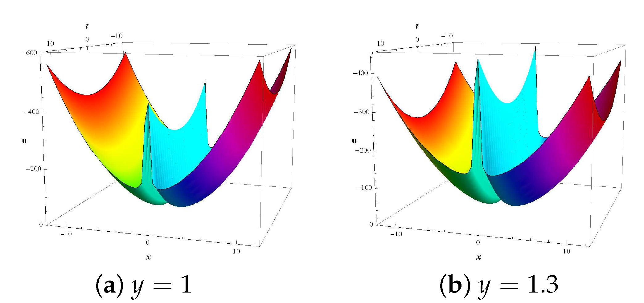
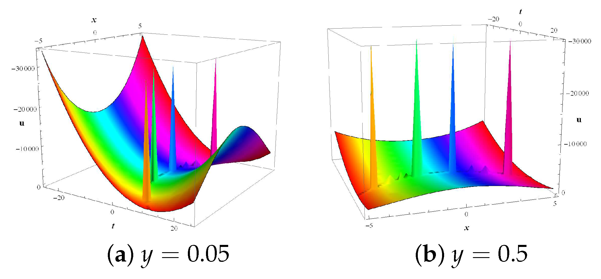
4. Graphical Illustrations for Soliton Solutions

The dynamical structures of mathematical expressions can be made more predictable through their graphical representation. The physical interpretation of the explicit solutions is very beneficial in explaining the physically meaningful behavior of the system. It also provides vital information/evidence to understand nonlinear phenomena physically. Numerical simulations have been carried out to exhibit the best perspective views of graphical representation results. Solitons are solitary wave packets and are known for their elastic scattering property that they do not change their shapes and amplitudes after the mutual collision. In addition, they play a conventional role in the wave-propagation of light in optical fibers, optical engineering, and many other phenomena in plasma and nonlinear dynamics. In the present section, we have analyzed the constructed solutions (23), (32), (41) of the first variable coefficient KP Equation (2) and solutions (71), (93), (102), (111) of the second variable coefficient KP Equation (3) by their three-dimensional dynamical structures. The best choices of arbitrary constant parameters and independent functions contribute to the development of physically meaningful profiles. Finally, the dynamical structures of 3D graphics are as follows:

Figure 1 shows oscillatory multi-wave solitons are observed for the expression (23). This graphical representation is obtained by taking suitable values to the arbitrary constants as $B_3=0.031$ and $g\left(t\right)=\frac{1}{t^2-5t+6}$ for $-5\le x\le 5$ and $1\le t\le 4.$

Figure 2 depicts curved-shaped multi-wave solitons behavior for the expression (32). The appropriate values of introduced arbitrary constants are taken as $b_1=0.05$, $b_2=0.03$, $b_3=0.05$, and arbitrary function as $g\left(t\right)=t^2,$ for $-25\le x\le 15$, $-15\le t\le 15$. The study of solitary waves has a extensive applications in many fields such as oceanographic engineering, non-linear optics etc.

Figure 3 demonstrates the elastic behavior of multi-solitons structures of solution (41). The profiles are illustrated by taking the particular values of parameters as $b_2=-4$, for $-10\le x\le 10$, $-10\le y\le 10$, $F_1\left(t\right)=t^2$ and $g\left(t\right)=t^2$.

Figure 4 reveals two different W-formed solitons in 3D-forms of solution (71) that was observed by numerical simulation for $-12\le x\le 12$, $-12\le t\le 12$, $b_1=5.05$, $b_2=0.001$, $b_3=0.5$ and $h\left(t\right)=t^2$.

Figure 5 shows the interactions between periodic multi-wave solutions and diverse solitons by setting arbitrary constants as $b_2=0.4$, $b_3=0.33$ and function as $h\left(t\right)=\frac{1}{t-4}$ in the particular solution (93). These two figures are traced at $t=1$ and $t=11$ for $-20\le x\le 15$, $-40\le y\le 45$. These figures show interaction between parabolic and multi-solitons behaviour in the spatial profile.

Figure 6: Annhilations of curved-quadruple four-solitons profiles are exhibited for the solution given by Equation (102). The profiles shoh four-soliton solitons structures by choosing the adequate values of arbitrary function as $f_3\left(t\right)$ = t, $h\left(t\right)=t^2$ and remaining parameters as $b_1=5.05$, $b_2=1.5$ and $b_3=1.5$. This profile is traced at $y=0.05$, and $y=0.5$ for $-25\le x\le 25$, $-5\le t\le 5$.

Figure 7 represents the nonlinear wave profiles of Equation (111) in 3D-graphics. Attractive intersections of oscillatory multi-solitons are observed in this figure of u at $t=0.5$ and $t=1.4$$\forall -10\le x\le 10$, $-10\le y\le 10$. This profiles are traced by taking the values of constants as $a=0.005$, $b_2=21.001$, $b_3=0.003$ and arbitrary function as $f_3\left(t\right)=t^4$.

5. Conclusions and Discussion

In summary, the two novel variable coefficients KP equations in (2+1)-dimensions are studied. Lie symmetries, infinitesimal generators, invariance’s criterion, and potential vector fields are presented. The Lie group of transformation technique is employed to derive the two stages of similarity reductions of VCKP equations. Subsequently, some exact invariant solutions are achieved in the forms of dark and bright solitons, multi-wave solitons, curved-shaped multiple solitons, double W-shaped solitons, and novel solitary wave solitons. All the newly established solutions have not been studied in previous literature. These precise solutions involve arbitrary independent functional parameters and other constants capable of revealing the important dynamical structures of nonlinear KP equations and shallow water wave models. It is important to note that the solutions obtained can be applied to nonlinear water wave models, nonlinear dynamics, optical physics, optical engineering, plasma physics, ion-acoustics physics, soliton theory, and other fields. In conclusion, the presented Lie symmetry technique that we implemented is affirmed by its reliability, trustworthiness, and productivity to solve analytically. This investigation is greatly suggested for the betterment of advanced research.

References

1. Guan, X.; Liu, W.; Zhou, Q.; Biswas, A. Darboux transformation and analytic solutions for a generalized super-NLS-mKdV equation. Nonlinear Dyn. 2019, 98, 1491–1500. [Google Scholar] [CrossRef]
2. Constantin, A.; Ivanov, R.I.; Lenells, J. Inverse scattering transform for the DegasperisProcesi equation. Nonlinearity 2010, 23, 2559. [Google Scholar] [CrossRef] [Green Version]
3. Kumar, S.; Mohan, B. A study of multi-soliton solutions, breather, lumps, and their interactions for kadomtsev–Petviashvili equation with variable time coeffcient using hirota method. Phys. Scr. 2021, 96, 125255. [Google Scholar] [CrossRef]
4. Ma, W.X.; Fan, E. Linear superposition principle applying to Hirota bilinear equations. Comput. Math. Appl. 2011, 61, 950–959. [Google Scholar] [CrossRef] [Green Version]
5. Kudryashov, N.A. Simplest equation method to look for exact solutions of nonlinear differential equations. Chaos Solitons Fract. 2005, 24, 1217–1231. [Google Scholar] [CrossRef] [Green Version]
6. Shen, Y.J.; Gao, Y.T.; Yu, X.; Meng, G.Q.; Qin, Y. Bell-polynomial approach applied to the seventh-order Sawada-Kotera-Ito equation. Appl. Math. Comput. 2014, 227, 502–508. [Google Scholar] [CrossRef]
7. Zayed, E.M.; Shohib, R.M. Optical solitons and other solutions to Biswas-Arshed equation using the extended simplest equation method. Optik 2019, 185, 626–635. [Google Scholar] [CrossRef]
8. Ebaid, A.; Aly, E.H. Exact solutions for the transformed reduced Ostrovsky equation via the F-expansion method in terms of Weierstrass-elliptic and Jacobian-elliptic functions. Wave Motion 2012, 49, 296–308. [Google Scholar] [CrossRef]
9. Lou, S.Y.; Hu, X.; Chen, Y. Nonlocal symmetries related to Bäcklund transformation and their applications. J. Phys. A Math. 2012, 45, 155209. [Google Scholar] [CrossRef] [Green Version]
10. Nisar, K.S.; Ilhan, O.A.; Abdulazeez, S.T.; Manafian, J.; Mohammed, S.A.; Osman, M.S. Novel multiple soliton solutions for some nonlinear PDEs via multiple Exp-function method. Result Phys. 2021, 21, 103769. [Google Scholar] [CrossRef]
11. Ali, K.K.; Wazwaz, A.M.; Osman, M.S. Optical soliton solutions to the generalized nonautonomous nonlinear Schrödinger equations in optical fibers via the sine-Gordon expansion method. Optik 2020, 208, 164132. [Google Scholar] [CrossRef]
12. Sulaiman, T.A.; Yusuf, A.; Abdel-Khalek, S.; Bayram, M.; Ahmad, H. Nonautonomous complex wave solutions to the (2+1)-dimensional variable-coefficients nonlinear Chiral Schrödinger equation. Result Phys. 2020, 19, 103604. [Google Scholar] [CrossRef]
13. Niwas, M.; Kumar, S.; Kharbanda, H. Symmetry analysis, closed-form invariant solutions and dynamical wave structures of the generalized (3+1)-dimensional breaking soliton equation using optimal system of Lie subalgebra. J. Ocean Eng. Sci. 2021. [Google Scholar] [CrossRef]
14. Wazwaz, A.M. Two new integrable Kadomtsev–Petviashvili equations with time-dependent coefficients: Multiple real and complex soliton solutions. Waves Random Complex Media 2020, 30, 776–786. [Google Scholar] [CrossRef]
15. Tian, S.F.; Zhang, H.Q. On the integrability of a generalized variable-coefficient forced Korteweg-de Vries equation in fluids. Stud. Appl. Math. 2014, 132, 212–246. [Google Scholar] [CrossRef]
16. Chen, S.; Zhou, Y.; Baronio, F.; Mihalache, D. Special types of elastic resonant soliton solutions of the Kadomtsev–Petviashvili II equation. Rom. Rep. Phys. 2018, 70, 102–118. [Google Scholar]
17. Kadomtsev, B.B.; Petviashvili, V.I. On the stability of solitary waves in weakly dispersive media. Sov. Phys. Dokl. 1970, 15, 539–541. [Google Scholar]
18. Hereman, W.; Nuseir, A. Symbolic methods to construct exact solutions of nonlinear partial differential equations. Math. Comput. Simul. 1997, 43, 13–27. [Google Scholar] [CrossRef]
19. Liu, J.G.; Zhu, W.H. Multiple rogue wave, breather wave and interaction solutions of a generalized (3+1)-dimensional variable-coefficient nonlinear wave equation. Nonlinear Dyn. 2021, 103, 1841–1850. [Google Scholar] [CrossRef]
20. Baldwin, D.E.; Hereman, W. A symbolic algorithm for computing recursion operators of nonlinear partial differential equations. Int. J. Comput. Math. 2010, 87, 1094–1119. [Google Scholar] [CrossRef] [Green Version]
21. Clarkson, P.A.; Winternitz, P. Nonclassical symmetry reductions for the Kadomtsev–Petviashvili equation. Physica D 1991, 49, 257–272. [Google Scholar] [CrossRef]
22. Kumar, M.; Tanwar, D.V.; Kumar, R. On Lie symmetries and soliton solutions of (2+1)-dimensional Bogoyavlenskii equations. Nonlinear Dyn. 2018, 94, 2547–2561. [Google Scholar] [CrossRef]
23. Kassem, M.M.; Rashed, A.S. N-solitons and cuspon waves solutions of (2+1)-dimensional Broer-Kaup-Kupershmidt equations via hidden symmetries of Lie optimal system. Chin. J. Phys. 2018, 57, 90–104. [Google Scholar] [CrossRef]
24. Tanwar, D.V. Optimal system, symmetry reductions and group-invariant solutions of (2+1)-dimensional ZK-BBM equation. Phys. Scr. 2021, 96, 065215. [Google Scholar] [CrossRef]
25. Laouini, G.; Amin, A.M.; Moustafa, M. Lie Group Method for Solving the Negative-Order Kadomtsev-Petviashvili Equation (nKP). Symmetry 2021, 13, 224. [Google Scholar] [CrossRef]
Figure 1. Two mixed dynamical structures of solitary waves and oscillatory multi-wave solitons for solution (23) with parameter a = 1 , b = 5 , , c = 6 , B 3 = 0.031 and g ( t ) = 1 a t 2 + b t + c .
Symmetry 14 00597 g001
Figure 2. Two mixed dynamical structures of curved type multi- solitons for solution (32) with parameters b 1 = 0.05 , b 2 = 0.03 , b 3 = 0.05 , and g ( t ) = t 2 .
Symmetry 14 00597 g002
Figure 3. Two mixed dynamical structures of curved-form multi-wave solitons for solution (41) with parameters b 2 = 4 , g ( t ) = t 2 and F 1 ( t ) = t 2 .
Symmetry 14 00597 g003
Figure 4. Two mixed dynamical structures of double W-shaped solitons with parabolic waves for solution (71) with parameters b 1 = 5.05 , b 2 = 0.001 , b 3 = 0.5 and h ( t ) = t 2 .
Symmetry 14 00597 g004
Figure 5. Two mixed dynamical structures of interactions between solitary waves and oscillating multi-peakon solitons for solution (93) with parameters b 2 = 0.4 , b 3 = 0.33 and h ( t ) = 1 t 4 .
Symmetry 14 00597 g005
Figure 6. Two mixed dynamical structures of curved-shaped quadruple (four) solitons for solution (102) with parameters b 1 = 5.05 , b 2 = 1.5 , b 3 = 1.5 , f 3 ( t ) = t and h ( t ) = t 2 .
Symmetry 14 00597 g006
Figure 7. Two mixed dynamical structures of oscillatory periodic multiwave-solitons for solution (111) with parameters a = 0.005 , b 2 = 21.001 , b 3 = 0.003 and f 3 ( t ) = t 4 .
Symmetry 14 00597 g007
Publisher’s Note: MDPI stays neutral with regard to jurisdictional claims in published maps and institutional affiliations.