Fast Computation of Highly Oscillatory ODE Problems: Applications in High-Frequency Communication Circuits

Abstract

The paper demonstrates symmetric integral operator and interpolation based numerical approximations for linear and nonlinear ordinary differential equations (ODEs) with oscillatory factor $x^{\prime }=\psi \left(x\right)+{\chi }_{\omega }\left(t\right)$, where the function ${\chi }_{\omega }\left(t\right)$ is an oscillatory forcing term. These equations appear in a variety of computational problems occurring in Fourier analysis, computational harmonic analysis, fluid dynamics, electromagnetics, and quantum mechanics. Classical methods such as Runge–Kutta methods etc. fail to approximate the oscillatory ODEs due the existence of oscillatory term ${\chi }_{\omega }\left(t\right)$. Two types of methods are presented to approximate highly oscillatory ODEs. The first method uses radial basis function interpolation, and then quadrature rules are used to evaluate the integral part of the solution equation. The second approach is more generic and can approximate highly oscillatory and nonoscillatory initial value problems. Accordingly, the first-order initial value problem with oscillatory forcing term is transformed into highly oscillatory integral equation. The transformed symmetric oscillatory integral equation is then evaluated numerically by the Levin collocation method. Finally, the nonlinear form of the initial value problems with an oscillatory forcing term is converted into a linear form using Bernoulli’s transformation. The resulting linear oscillatory problem is then computed by the Levin method. Results of the proposed methods are more reliable and accurate than some state-of-the-art methods such as asymptotic method, etc. The improved results are shown in the numerical section.

1. Introduction

Accurate computation of the initial value problems with oscillatory forcing term (IVPs) is one of the ambitious task in scientific computing. In this work, we focused on a particular case of the IVPs involving an ODE system

$${\mathbf{x}}^{\prime }\left(t\right)=\mathbf{B}\mathbf{x}\left(\mathbf{t}\right)+h_{\omega }\left(t\right)\mathbf{f}\left(\mathbf{x}\left(t\right)\right),t\ge 0,\mathbf{x}\left(0\right)={\mathbf{x}}_0\in {\mathbb{R}}^n,$$

(1)

where $\mathbf{B}$ is a square matrix of order n, $\mathbf{f}\left(\mathbf{x}\right(t\left)\right)$ is a n-vector of functions, and $h_{\omega }\left(t\right)$ is a rapidly oscillating scaler function with a frequency parameter $\omega \gg 1$. Particularly, we assume $h_{\omega }\left(t\right)=e^{i\omega g\left(t\right)}$. Initial value problem (1) is the simplest model of the more complicated problems of electronic engineering. Generally, nonlinear ODEs and differential algebraic equations (DAEs) with oscillatory forcing term are frequently appeared in this field. The analytic solution of the ODEs (1) in terms of symmetric integral operator and is given as

$$\mathbf{x}=e^{\mathbf{A}t}{\mathbf{x}}_0+\mathcal{L}\left(f\right),t\ge 0,$$

(2)

where $\mathcal{L}\left(f\right)=e^{\mathbf{A}t}{\int }_0^t{e}^{-\mathbf{A}z}\mathbf{f}\left(\mathbf{x}\left(z\right)\right)h_{\omega }\left(z\right)dz$ [1]. In this paper, we consider that the phase function $h_{\omega }\left(t\right)$ has no stationary point for $t\ge 0$.

High-frequency transmissions are regularly encountered in the field of radio frequency. This is a result of modulation, which allows a lower-frequency information stream to be imposed on a higher-frequency carrier. The goal is to make it possible to implement audio transmission using antennae that are reasonable in size. If modulation is not used, long-distance antennas on the order of several hundred miles to several thousand miles are necessary. When it comes to radio frequency communication systems, transmissions with frequencies in the Mega Hertz range and above are typical. Because of the existence of solid-state amplifiers, mixers, and other components in radio frequency transmission systems, the nonlinearity of the system might occur [2].

In most radio frequency systems, the linear part of (1) appears because linear indicators, i.e., resistors, and capacitors are used in conjunction with the system. While the nonlinear portion is caused by amplifiers, mixers, or nonlinear controlled resistors and capacitors. The linear portion is caused by a combination of these components. ODEs (1) is a straight forward model containing nonlinearity. The emergence of the phase $e^{\lambda }sin\left(\omega t\right)$ is due to the application of sine waves to the terminals of circuits including diodes or transistors, which causes the term to appear. It is important to note that sinusoids and amplifiers employing transistors are ubiquitous in indication systems and should not be overlooked [2,3,4].

As a result of the ongoing rapid changes in the radio frequency and telecommunications industries, we must build faster simulations, faster designs, and faster product outputs to keep up with the times. It is necessary to update the existing computer aided design (CAD) tools in order to accommodate the new algorithms. Furthermore, the increasing complexity of modulation formats makes it unreasonably slow to interpret software tools, resulting in dissatisfaction with the end output. It is now imperative that rapid and precise numerical techniques be developed in order to deal with the situation.

Many well-known researchers have made significant contributions to this field, recognizing the importance of these issues and the frequency with which they are encountered in many domains of science and engineering. A number of rapid approaches, such as the Runge–Kutta method of order 4, multistep methods, such as the Adam–Bashforth method and the Adam–Moulton method [5,6], as well as several other advanced numerical methods, were proposed to estimate IVPs (1). When Taylor’s series was used to reduce multistep methods to single-step methods, and then Newton-Cotes quadrature was employed to approximate the ODEs, and the result was cited as [7].

Fast numerical procedures [8,9] have been derived for evaluation of rapidly oscillatory ordinary differential equations. Recently, the state-of-the-art numerical methods, i.e., asymptotic and Filon-types of methods, have been implemented to approximate highly oscillatory linear and nonlinear ODEs [1]. The generalized Filon’s method is used to solve stochastic differential equations and extendable to evaluate ordinary differential equations with rapidly oscillating factors [10].

In [1], the oscillatory IVPs are transformed to highly oscillatory integrals with Fourier kernel. The integrals are evaluated numerically by some state-of-the-art methods such as the Levin collocation method [11,12,13,14,15,16,17], asymptotic method [18,19,20], numerical steepest decent method [21,22], and Filon(-type) methods [1,23,24,25,26,27].

In [10], the authors presented generalized Filon quadrature to evaluate a first-order stochastic differential equation with rapidly oscillating factor. The method is applicable to solve a variety of oscillatory ODE problems. Recently, the authors [28] constructed a multivalue mixed collocation method based on generalized Hermite polynomials for numerical solution of oscillatory ODEs system. Some theoretical results are also derived in the paper.

The motivation is made from the work [1], in which the integral is evaluated by the asymptotic method. Levin collocation method is one of the accurate tool which can evaluate oscillatory integrals with complicated phase function, where the asymptotic method fails. Secondly, radial basis function interpolation is one of the best approximation techniques which accurately approximates irregular oscillatory function. The Levin collocation method based on multiquadric RBF is implemented in this work to solve the oscillatory-type linear ODEs. The method improves accuracy with the inverse power of $\omega$. The method is applicable to oscillatory problems with stationary free phase functions. Moreover, the integrand in (2) is interpolated by the RBF collocation method instead of the Newton backward interpolant, following the multistep methods and evaluated the integral by quadrature methods or matlab built-in code "quadv". Finally, a nonlinear IVPs (1) can be transformed into linear IVPs by Bernoulli’s transformation and then approximated by the proposed algorithms.

2. Numerical Procedures

In this section, we discuss two numerical techniques for solution of oscillatory and nonoscillatory ODEs. According to the first method, the integrand of (2) is interpolated by the RBF collocation method, and then the integral is evaluated by the built-in code of MATLAB programming ‘quadv’ or uses multi-resolution quadratures to approximate the targeted integral. The method accurately approximates the nonoscillatory linear ODEs. Secondly, a generic method is implemented to approximate both nonoscillatory and highly oscillatory linear ODEs. The Levin collocation method based on multiquadric RBFs is used to approximate the oscillatory integral of the ODE solution (2). Finally, nonlinear ODEs are transformed to linear ODEs and then approximated by the proposed procedures.

2.1. Procedure Based on RBF Interpolation

A modified form of IVP (1) is given as

$$x^{\prime }\left(t\right)=G(t,x),t\in [\alpha ,\beta ],x\left(\alpha \right)=x_0.$$

(3)

By the Euler method, the exact solution of ODE (3) can be written as

$$x\left(t\right)=x_0+{\int }_{\alpha }^{t}G(t,x)\mathrm{d}t,t\in [\alpha ,\beta ].$$

(4)

On descritization over the intervals $[t_i,t_{i+1}]$, (4) is reduced to

$$x\left(t_{i+1}\right)=x\left(t_i\right)+{\int }_{t_i}^{t_{i+1}}G(t,x)\mathrm{d}t,i=0,1,\dots ,N.$$

(5)

Now, we interpolate the integrand $G(t,x)$ by the RBF collocation method. The unknown values $x\left(t\right)$ of the integrand can be predicted by the RK4 method.

The global RBFs $\psi (\mathfrak{r},\rho )$ are univariate smooth functions with a free shape parameter $\rho$. The accuracy and shape of the RBF interpolation depend upon the optimal value of $\rho$. For a given set of m-centers, $t_i={\nu }_0<{\nu }_1<\dots <{\nu }_m=t_{i+1}$, an approximate function $\widehat{\mathcal{Q}}\left(\nu \right)={\sum }_{j=0}^m{\lambda }_j\psi (\mathfrak{r},\rho ),\mathfrak{r}=\left|\right|\nu -{\nu }_j{\left|\right|}_2,j=0,1,\dots m,$ is supposed to satisfy the following interpolation condition:

$$\mathcal{Q}\left({\nu }_k\right)=G({\nu }_k,x_k),k=0,1,\dots ,m,$$

The equation confers a system of linear equations, and can be written in matrix form as

$$\mathbf{B}\lambda =\mathbf{G},$$

(6)

By solving linear equation’s system, (6), the unknown coefficients, ${\lambda }_j$ could easily be found out. The matrix ${\mathbf{B}}_{m\times m}$ is a square matrix called system matrix, and $\lambda$ and $\mathbf{G}$ are m-vectors. The entries of ${\mathbf{B}}_{m\times m}$ are given as

$$B_{k,j}=\psi \left(\right||({\nu }_k-{\nu }_j){,\rho \left|\right|}_2),k,j=0,1,...,m.$$

Thus, Equation (5) becomes

$$x\left(t_1\right)=x\left(t_0\right)+{\int }_{{\nu }_j}^{{\nu }_{j+1}}\sum _{j=1}^m{\left(B^{-1}\mathbf{G}\right)}_j\psi \left|\right|(\nu -{\nu }_j),\rho {\left|\right|}_2\mathrm{d}\nu ,j=0,1,\dots m.$$

The integral can be numerically evaluated by the multiresolution quadratures such as hybrid functions or Haar wavelets [11,12,29]. It can also be evaluated by the MATLAB built-in codes such as quadgk, quadv, and quadl. In the current work, we have used “quadv” for evaluation of the targeted integral.

For optimal accuracy, we have chosen multiquadric RBF, $\varphi \left(r\right)=\sqrt{r^2+{\rho }^2}$, where $r=\left|\right|\nu -{\nu }_j{\left|\right|}_2>0$ are the radial distances and the free parameter $\rho$ is called shape parameter. An optimal value of $\rho$ is an open problem. In this work, we have taken a fixed value of $\rho$.

Now, the desired solution of (5) at $(j+1)$-th time level is given by

$$x\left(t_{i+1}\right)=x\left(t_i\right)+{\int }_{t_i}^{t_{i+1}}\sum _{j=1}^m{\left(B^{-1}\mathbf{G}\right)}_j\psi \left|\right|(\nu -{\nu }_j),\rho {\left|\right|}_2\mathrm{d}\nu .$$

For each $i=0,1,\dots ,N$, the integral can be evaluated recursively by the RBF collocation method, and the numerical results can be obtained at different time levels.

2.2. Levin Collocation Method

This method is efficiently implementable to evaluate nonoscillatory ODEs and the ODEs with highly oscillatory forcing term $h_{\omega }\left(t\right)$. The initial value problem (1) can be reduced to a single ODE as

$$x^{\prime }\left(t\right)=Ax\left(t\right)+e^{i\omega g\left(t\right)},t\ge 0,x\left(0\right)=x_0\in \mathbb{R},$$

(7)

with analytical solution

$$x\left(t\right)=e^{At}x\left(t_0\right)+e^{At}{\int }_0^t{e}^{-A\tau }{e}^{i\omega g\left(\tau \right)}\mathrm{d}\tau ,$$

(8)

where A is assumed as a constant parameter for single ODE [30]. In the current work, we also assume that $g^{\prime }\left(t_0\right)\ne 0$ for any $t_0\in [0,t]$ and $\omega \gg 1$. The descretized form of (8) is given by

$$x\left(t_{i+1}\right)=e^{A{t}_i}x\left(t_i\right)+e^{A{t}_i}{\int }_{t_i}^{t_{i+1}}{e}^{-At}{e}^{i\omega g\left(t\right)}\mathrm{d}t,i=0,1,2,\dots ,N.$$

(9)

In order to approximate highly oscillatory integral ${\int }_{t_i}^{t_{i+1}}{e}^{-At}{e}^{i\omega g\left(t\right)}\mathrm{d}t$, we focus on the Levin quadrature theory which is briefly discussed as:

According to the Levin approach, an approximate function $\widehat{\mathcal{Q}}\left(t\right)={\sum }_{j=0}^m{\delta }_j\psi (\mathfrak{r},\rho )$ is supposed to be a solution of the following ordinary differential equation

$${\mathcal{Q}}^{\prime }\left(t\right)+i\omega g^{\prime }\left(t\right)\mathcal{Q}\left(t\right)=e^{-At}.$$

(10)

Integral on the right of (9) can be written as

$$\begin{array}{cc}\hfill {\int }_{t_i}^{t_{i+1}}{e}^{-At}{e}^{i\omega g\left(t\right)}\mathrm{d}t& ={\int }_{t_i}^{t_{i+1}}\left[{\widehat{\mathcal{Q}}}^{\prime }\left(t\right)-i\omega g^{\prime }\left(t\right)\widehat{\mathcal{Q}}\left(t\right))\right]e^{i\omega g\left(t\right)}\mathrm{d}t\hfill \\ \hfill & ={\int }_{t_i}^{t_{i+1}}d\left[\widehat{\mathcal{Q}}\left(t\right)e^{i\omega g\left(t\right)}\right]\hfill \\ & =\widehat{\mathcal{Q}}\left(t_{i+1}\right)e^{i\omega g\left(t_{i+1}\right)}-\widehat{\mathcal{Q}}\left(t_i\right)e^{i\omega g\left(t_i\right)}.\hfill \end{array}$$

(11)

Thus, the desired approximate solution of the IVP (7) is given as

$$x\left(t_{i+1}\right)=e^{A{t}_i}x\left(t_i\right)+e^{A{t}_i}\left[\widehat{\mathcal{Q}}\left(t_{i+1}\right)e^{i\omega g\left(t_{i+1}\right)}-\widehat{\mathcal{Q}}\left(t_i\right)e^{i\omega g\left(t_i\right)}\right],i=0,1,\dots ,N.$$

(12)

To find the approximate function $\widehat{\mathcal{Q}}\left(t\right)$, we substitute $\widehat{\mathcal{Q}}\left(t\right)={\sum }_{j=0}^m{\delta }_j\psi (\mathfrak{r},\rho )$ in the ODE (10), and by applying interpolation condition, we obtain

$$\sum _{j=0}^m{\delta }_j{\psi }^{\prime }({\mathfrak{r}}_k,\rho )+i\omega g^{\prime }\left(t_k\right)\sum _{j=0}^m{\delta }_j\psi ({\mathfrak{r}}_k,\rho )=e^{-A{t}_k},k=0,1,2,\dots ,M,$$

(13)

where $\psi (\mathfrak{r},\rho )=\sqrt{{\mathfrak{r}}^2+{\rho }^2},\mathfrak{r}=\left|\right|t-t_j{\left|\right|}_2,j=0,1,\dots ,m$ is the multi-quadric RBF and $\rho$ is the free shape parameter of the RBF interpolant.

Equation (13) also generates a linear equation’s system. This linear system of equations could be rewritten in the form of a matrix as

$$\mathbf{B}\delta =\mathbf{f},$$

or

$$\delta ={\mathbf{B}}^{-1}\mathbf{f}.$$

(14)

For $m=M$, the system matrix $\mathbf{B}$ becomes a square matrix with entries

$$b_{jk}={\psi }_j^{\prime }(\mathfrak{r},\rho )+i\omega g^{\prime }\left(t_k\right){\psi }_j(\mathfrak{r},\rho ).$$

(15)

By solving the system of linear Equation (14) by Gauss-elimination or LU-factorization method to obtain the unknown coefficients ${\delta }_j$, we can find, as a result, the approximate RBF solution $\widehat{\mathcal{Q}}\left(t\right)$. The desired solution of the ODE is obtain then by the Levin Formula (11) and is denoted by LCM.

2.3. Nonlinear Highly Oscillatory ODEs

In this section, we briefly describe a procedure that can transform Bernoulli-type nonlinear highly oscillatory ODEs to a linear form. Generally, the Bernoulli’s equation can be written as

$$x^{\prime }+p\left(t\right)x=g\left(t\right)x^{\alpha },\alpha \in R.$$

(16)

For $\alpha =0$ or $\alpha =1$, (16) is a linear ODE. Otherwise, we use the following transformation

$$u\left(t\right)={\left[x\left(t\right)\right]}^{1-\alpha }.$$

On differentiating, we obtain

$$u^{\prime }\left(t\right)=(1-\alpha )x^{-\alpha }{x}^{\prime }.$$

(17)

Substituting the value of $x^{\prime }$ from (16) in (17), we obtain

$$u^{\prime }\left(t\right)=(1-\alpha )x^{-\alpha }\left[g\left(t\right)x^{\alpha }-p\left(t\right)x\right],$$

or

$$u^{\prime }\left(t\right)=(1-\alpha )g\left(t\right)-(1-\alpha )p\left(t\right)x^{1-\alpha }.$$

On rearranging, we obtain

$$u^{\prime }+(1-\alpha )p\left(t\right)u=(1-\alpha )g\left(t\right).$$

(18)

The transformed ODE (18) is linear and can be approximated by the two proposed methods.

Theorem 1

([12]). Let $x_0$ be a stationary point of order $“p”$, and let $\vartheta ={\left(\frac{N}{10\omega }\right)}^{1/p}$, $\theta ={min}_{x\epsilon [\vartheta ,1]}\left|{\phi }^{\prime }\left(x\right)\right|$. Then, the following holds true:

i.

The error bound of the RBF method with Levin approach to approximate the oscillatory integral $I\left[\psi \right]={\int }_{\vartheta }^1\psi \left(x\right)e^{i\omega \phi \left(x\right)}\mathrm{d}x$ is given by

$$E_{abs}=\mid I\left[\psi \right]-Q_L^{mm}\mid =O\left(\frac{{(1-\vartheta )}^M}{{\left(\omega \right)}^{1/p}}\right),$$

(19)

for m collocation points.

ii.

For computation of $I\left[\psi \right]={\int }_{{\upsilon }_1}^1\psi \left(x\right)e^{i\omega \phi \left(x\right)}\mathrm{d}x$ by the same method at $-1<{\upsilon }_1<{\upsilon }_2<...<{\upsilon }_M=1$, the error bound is given by

$$E_{abs}=\mid I\left[\psi \right]-Q_L^{mm}\mid =O\left(\frac{{(1-{\upsilon }_1)}^{M-1}}{{\omega }^2}\right),$$

(20)

for $\omega \gg 1$.

Proof. 

See [12]. □

As shown in (12), solution by the Levin collocation method of the IVP (7) in the local domain $[t_i,t_{i+1}],i=0,1,...,N$ is given as

$$x\left(t_{i+1}\right)=e^{A{t}_i}x\left(t_i\right)+e^{A{t}_i}\left[\widehat{\mathcal{Q}}\left(t_{i+1}\right)e^{i\omega g\left(t_{i+1}\right)}-\widehat{\mathcal{Q}}\left(t_i\right)e^{i\omega g\left(t_i\right)}\right],i=0,1,...,N.$$

(21)

The error estimate of the method $LCM$ is demonstrated in (19). Thus, the desired error estimate in the local domain interval $[t_i,t_{i+1}]$ of the new method to compute IVP (7) is given by

$$E_{ivp}=O\left(\frac{{(1-t_i)}^M}{{\left(\omega \right)}^{1/p}}\right),\mathrm{for}\mathrm{each}{t}_i,i=0,1,...N-1.$$

(22)

For m collocation points, the error estimate (22) is reduced to

$$E_{ivp}=O\left(\frac{{(1-{\upsilon }_1)}^{m-1}}{{\omega }^2}\right),$$

(23)

where m represents the number of collocation points of the LCM. Thus, the asymptotic error estimate reach to $O\left({\omega }^{-2}\right)$.

3. Numerical Assessment

Few benchmark nonoscillatory and highly oscillatory IVPs have been considered from the literature to verify accuracy of the proposed procedures. The results of the new methods are compared with asymptotic method [1]. Accuracies are measured in terms of infinity norm $\left|\right|L_{\infty }\left|\right|$ and absolute errors $E_{abs}$. CPU time (in seconds) is also computed in some problems. The comparison of the new work is also performed with some classical methods such as RK4 and the Adam–Bashforth method in case of nonoscillatory ODEs.

Test Problem 1.Consider the following nonoscillatory ODE [5]

$$x^{\prime }\left(t\right)=x\left(t\right)-t^2+1,x\left(0\right)=0.5,t\in [0,2],$$

(24)

with analytical solution

$$x\left(t\right)={(1+t)}^2-0.5e^t.$$

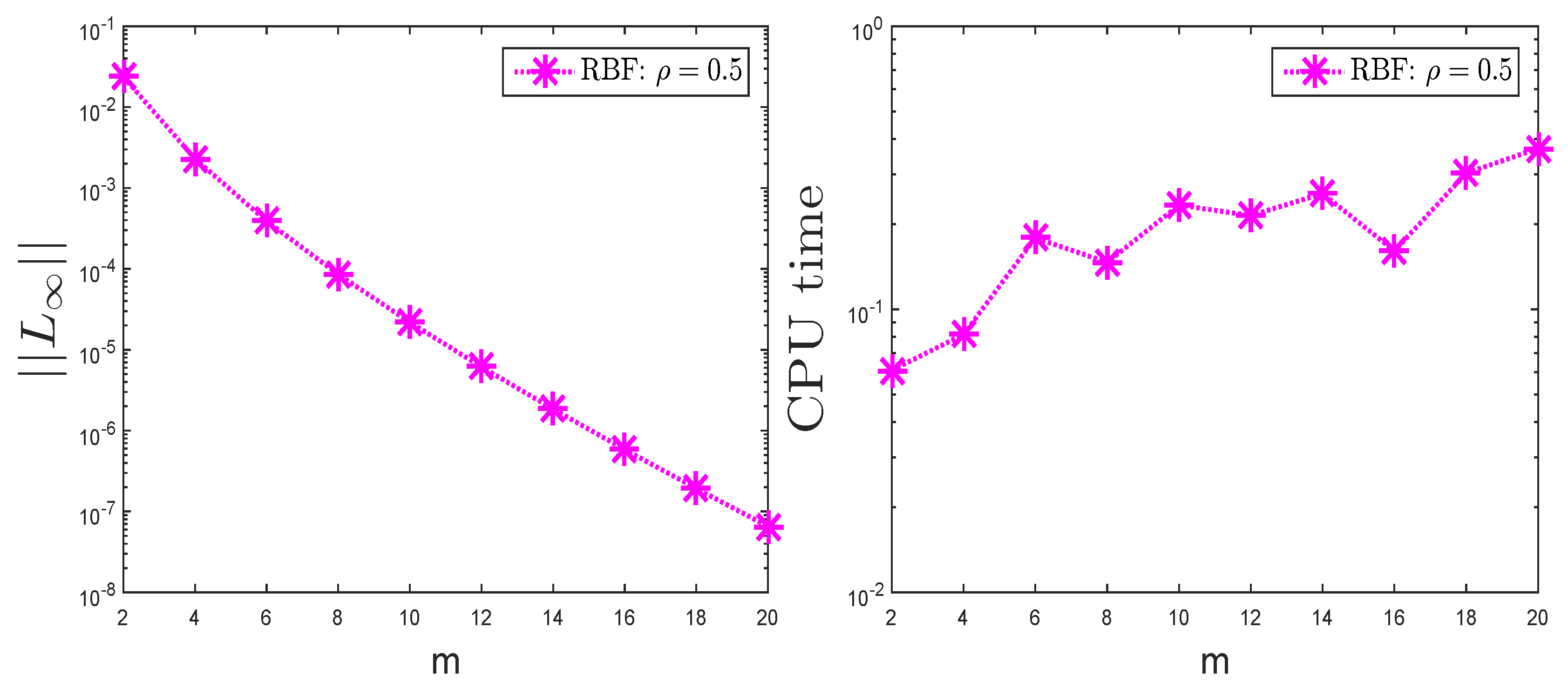
The ODE (24) is evaluated numerically by the AF4, RK4, and the proposed RBF collocation methods. The results at different time levels in terms of $E_{abs}$ and $L_{\infty }$ are calculated and analyzed in

Table 1. Test Problem 1, $E_{abs}$ produced by AF4, RK4 [5] and RBF method for $m=10$ and $\rho =2.5$.

t	AF4	RK4	RBF
0	−	−	−
$0.2$	−	$5.30\times {10}^{-6}$	$6.80\times {10}^{-7}$
$0.4$	−	$1.14\times {10}^{-5}$	$5.29\times {10}^{-7}$
$0.6$	−	$1.86\times {10}^{-5}$	$5.89\times {10}^{-7}$
$0.8$	$8.28\times {10}^{-5}$	$2.69\times {10}^{-5}$	$5.52\times {10}^{-7}$
$1.0$	$2.22\times {10}^{-4}$	$3.64\times {10}^{-5}$	$5.82\times {10}^{-7}$
$1.2$	$4.07\times {10}^{-4}$	$4.74\times {10}^{-5}$	$5.47\times {10}^{-7}$
$1.4$	$6.60\times {10}^{-4}$	$5.99\times {10}^{-5}$	$5.99\times {10}^{-7}$
$1.6$	$1.01\times {10}^{-3}$	$7.43\times {10}^{-5}$	$4.89\times {10}^{-7}$
$1.8$	$1.48\times {10}^{-3}$	$9.06\times {10}^{-5}$	$8.34\times {10}^{-7}$
$2.0$	$2.11\times {10}^{-3}$	$1.06\times {10}^{-4}$	$1.15\times {10}^{-6}$

and Figure 1. It is shown in the table that the proposed method performs better than the other classical methods. The result of the RBF method depends upon the values of shape parameter $\rho$ and collocation points m as shown in Figure 1 (left). We see better accuracy on increasing the collocation points m. The CPU time (in seconds) of the proposed method is shown in Figure 1 (right). It is obvious from the results analyzed in the table and the figure that the RBF method improves the results for increasing m at low computational time.

Test Problem 2.Consider the following nonoscillatory ODE

$$x^{\prime }\left(t\right)=t-2x\left(t\right),x\left(0\right)=1,t\in [0,2],$$

(25)

with analytical solution

$$x\left(t\right)=\frac{1}{4}\left(2t-1+5e^{-2t}\right).$$

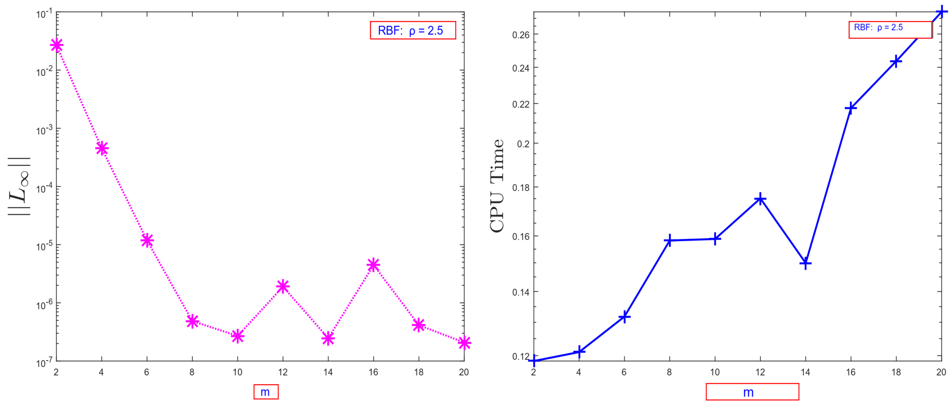
The ODE (25) is approximated by the RBF collocation method and the classical methods. Numerical results are analyzed in

Table 2. Test Problem 2, $E_{abs}$ produced by RBF and RK4 methods at $m=10$.

t	0.2	0.4	0.6	0.8	1
$RBF$	$5.03\times {10}^{-6}$	$1.51\times {10}^{-6}$	$1.18\times {10}^{-6}$	$7.59\times {10}^{-7}$	$2.22\times {10}^{-6}$
$RK4$	$9.99\times {10}^{-5}$	$1.34\times {10}^{-4}$	$1.35\times {10}^{-4}$	$1.20\times {10}^{-4}$	$1.01\times {10}^{-4}$

and Figure 2. From Figure 2 (left), it is shown that the proposed method improves accuracy on increasing m at fixed free shape parameter $\rho =2.5$. The CPU time comparison (in seconds) of the new method is shown in Figure 2 (right). This demonstrates that the new method decreases the errors on increasing the collocation points.

The results of the new method for fixed m and $\rho$ are compared with RK4 at different time levels and are shown in Table 2. It is evidence that the proposed method is accurate and efficient even at fewer nodal points.

Test Problem 3.Consider the following highly oscillatory IVP [1]

$$x^{\prime }=-x+\frac{1}{2}cos\left(\omega t\right),t\ge 0,x\left(0\right)=1.$$

The analytical solution obtained by MAPLE 16 is given as

$$x\left(t\right)=\frac{1}{2}cos\left(\omega t\right)+e^t(1-\frac{1}{2}cos\left(\omega t\right)).$$

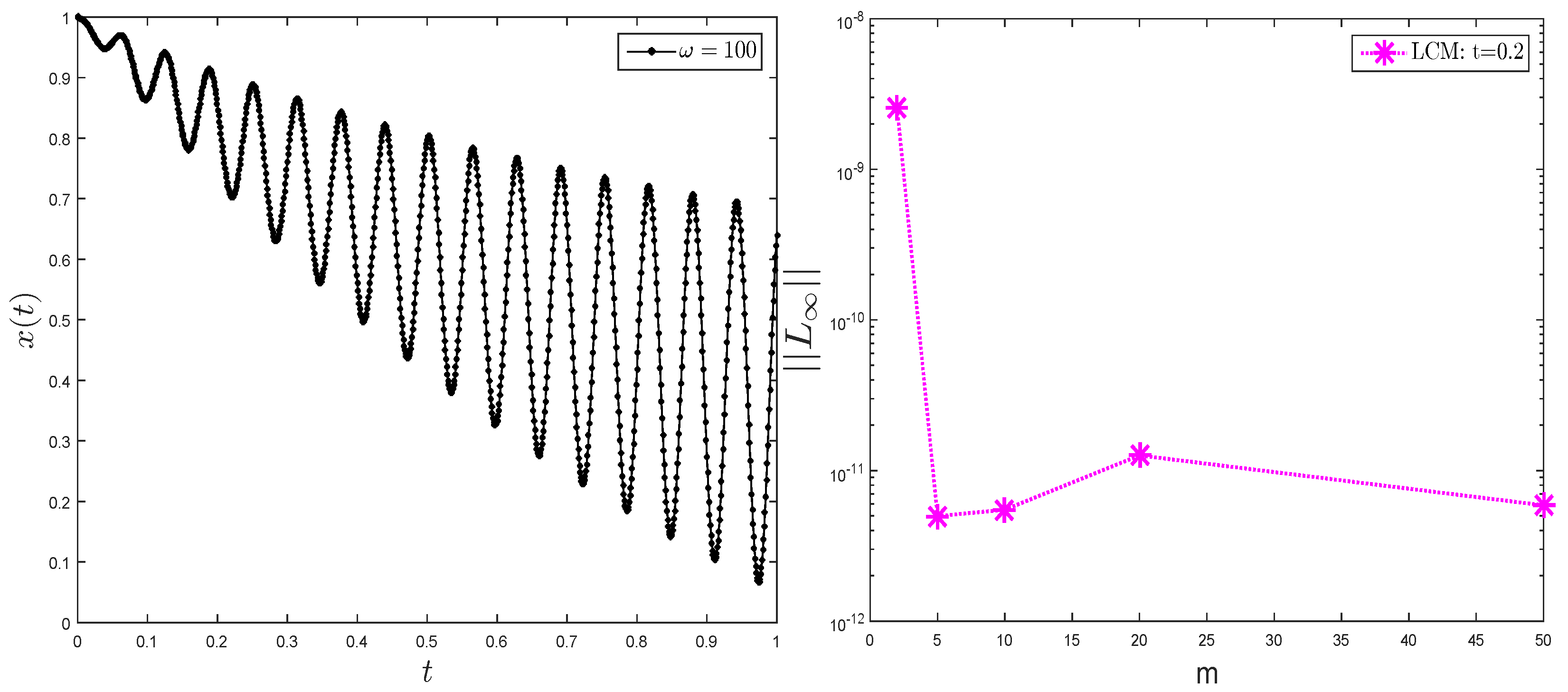
The given ODE is highly oscillatory. The irregular oscillations of the analytical solution are shown in Figure 3 (left) for $\omega =100$. The highly oscillatory IVP is hard to solve by the classical numerical methods such as RK4 and AF4 for higher values of $\omega$. The oscillatory problem is computed by the proposed Levin collocation method (LCM). Numerical results by the proposed method are compared with the asymptotic method [1] as shown in

Table 3. Test Problem 3, $E_{abs}$ produced by the LCM for $m=10$ and $Q_A^{Ai}$[1] for $\omega ={10}^3$.

t	0.2	0.4	0.6	0.8	1
$LCM$	$4.97\times {10}^{-12}$	$7.29\times {10}^{-11}$	$1.22\times {10}^{-11}$	$5.01\times {10}^{-11}$	$3.60\times {10}^{-10}$
$Q_A^{Ai}$[1]	$4.36\times {10}^{-10}$	$4.26\times {10}^{-10}$	$2.13\times {10}^{-11}$	$4.46\times {10}^{-10}$	$4.13\times {10}^{-10}$

. The table demonstrates that the new method is more accurate and faster than the asymptotic method for higher values of $\omega$. The method is tested for lager collocation points m on increasing values of $\omega$. The results are analyzed in

Table 4. Test Problem 3, $E_{abs}$ produced by the LCM for $t=0.2$.

$\mathit{\omega }/\mathit{m}$	2	5	10
1	$4.07\times {10}^{-7}$	$5.98\times {10}^{-9}$	$1.42\times {10}^{-9}$
10	$4.92\times {10}^{-6}$	$9.76\times {10}^{-11}$	$2.50\times {10}^{-11}$
100	$4.76\times {10}^{-7}$	$4.30\times {10}^{-11}$	$7.43\times {10}^{-11}$
500	$1.32\times {10}^{-9}$	$3.29\times {10}^{-11}$	$3.45\times {10}^{-11}$
1000	$2.57\times {10}^{-9}$	$4.97\times {10}^{-12}$	$5.49\times {10}^{-12}$

.

The method is also implemented at different time levels on increasing m, and it obtained higher accuracies. The results are presented in

Table 5. Test Problem 3, $E_{abs}$ produced by the LCM for $\omega ={10}^3$.

$\mathit{t}/\mathit{m}$	2	5	10
$0.2$	$2.57\times {10}^{-9}$	$4.98\times {10}^{-12}$	$5.49\times {10}^{-12}$
$0.4$	$2.81\times {10}^{-8}$	$7.29\times {10}^{-11}$	$7.94\times {10}^{-11}$
$0.6$	$6.78\times {10}^{-8}$	$1.22\times {10}^{-11}$	$1.87\times {10}^{-11}$
$0.8$	$6.59\times {10}^{-8}$	$5.01\times {10}^{-11}$	$7.63\times {10}^{-11}$
1	$6.39\times {10}^{-9}$	$3.60\times {10}^{-10}$	$1.94\times {10}^{-11}$

. In addition, the results of the LCM for fixed time level and increasing m are shown in Figure 3 (right). We see that the new method improves accuracy on increasing m as well as $\omega$ at different time levels.

Test Problem 4.Consider the following nonlinear highly oscillatory IVP [10]

$$x^{\prime }\left(t\right)=x+x^2{e}^{i\omega t},x\left(0\right)=1,t\in [0,1].$$

(26)

Using Bernoulli’s transformation, the nonlinear ODE (26) is transformed into the linear form as

$$u^{\prime }\left(t\right)=-u\left(t\right)-e^{i\omega t}.$$

(27)

The analytical solution of (27) is given as

$$u\left(t\right)=-e^{i\omega t}+e^{-t}(1+e^{i\omega t}).$$

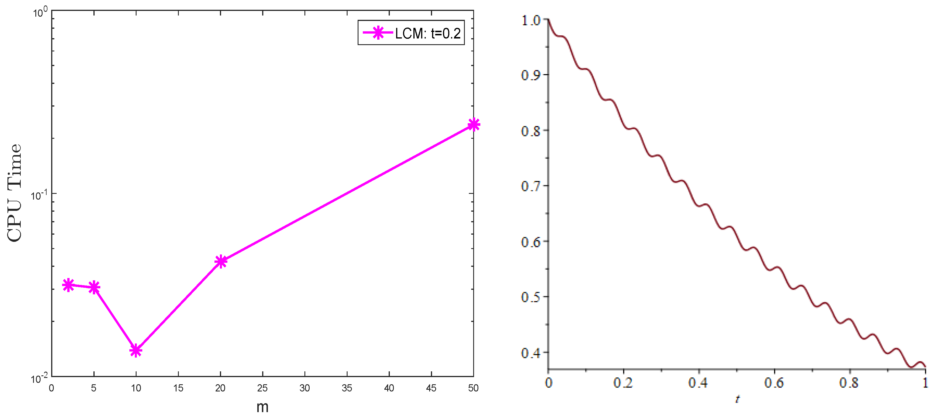
The transformed linear ODE (27) is computed by the new method LCM. Results and CPU time are analyzed in

Table 6. Test Problem 4, $E_{abs}$ produced by the LCM at fixed $t=0.2$.

$\mathit{\omega }/\mathit{m}$	2	5	10
1	$8.14\times {10}^{-7}$	$1.17\times {10}^{-8}$	$3.12\times {10}^{-9}$
10	$9.84\times {10}^{-6}$	$1.61\times {10}^{-10}$	$8.40\times {10}^{-11}$
100	$9.56\times {10}^{-7}$	$8.00\times {10}^{-11}$	$1.73\times {10}^{-11}$
500	$2.62\times {10}^{-9}$	$3.18\times {10}^{-11}$	$3.50\times {10}^{-11}$
1000	$5.11\times {10}^{-9}$	$4.38\times {10}^{-11}$	$4.49\times {10}^{-11}$

and

Table 7. Test Problem 4, $E_{abs}$ produced by the LCM at fixed $\omega ={10}^3$.

$\mathit{t}/\mathit{m}$	2	5	10
$0.2$	$5.11\times {10}^{-9}$	$4.38\times {10}^{-11}$	$4.49\times {10}^{-11}$
$0.4$	$5.59\times {10}^{-8}$	$6.10\times {10}^{-11}$	$4.81\times {10}^{-11}$
$0.6$	$1.35\times {10}^{-7}$	$6.54\times {10}^{-12}$	$1.95\times {10}^{-11}$
$0.8$	$1.31\times {10}^{-7}$	$5.16\times {10}^{-11}$	$9.29\times {10}^{-13}$
1	$1.28\times {10}^{-8}$	$6.34\times {10}^{-10}$	$4.68\times {10}^{-11}$

and Figure 4. Table 6 demonstrates that the new method improves the numerical results for increasing m and $\omega$. The proposed method is also examined for varying m at different time levels. Better results are obtained and are shown in Table 7.

The CPU time related to m is calculated and displayed in Figure 4 (left). We see that the new method is efficient as well. The exact solution of the oscillatory ODE is displayed in Figure 4 (right). From the whole discussion, it is obvious that the LCM is an accurate tool for approximating the oscillatory-type linear and nonlinear IVPs.

Test Problem 5.Consider the following highly oscillatory IVP [28]

$$x^{\prime }=-\left(x-sin\left(\omega t\right)\right)+\omega cos\left(\omega t\right),t\ge 0,x\left(0\right)=0,$$

(28)

with exact solution

$$x\left(t\right)=sin\left(\omega t\right).$$

The ODE (28) is highly oscillatory and is computed by the new method LCM. The results of the proposed method are compared with the multivalue collocation method reported in [28]. The absolute errors are analyzed in

Table 8. Test Problem 5, $\left|\right|L_{abs}\left|\right|$ produced by the LCM at $\omega ={10}^2$ and the method reported in [28].

Methods	${\mathit{h}}_1=1/40$	${\mathit{h}}_2=1/80$	${\mathit{h}}_3=1/160$	${\mathit{h}}_4=1/320$	${\mathit{h}}_5=1/640$
LCM	$2.12\times {10}^{-08}$	$8.74\times {10}^{-09}$	$1.88\times {10}^{-08}$	$8.98\times {10}^{-09}$	$2.07\times {10}^{-09}$
Multivalue CM [28]	$2.76\times {10}^{-01}$	$3.26\times {10}^{-02}$	$2.48\times {10}^{-09}$	$1.55\times {10}^{-04}$	$9.85\times {10}^{-06}$

, which demonstrates that the proposed method is better than the multivalue collocation method [28]. It is also shown in the table that the new method is highly accurate compared to the existing method [28].

4. Conclusions

In this paper, the RBF collocation method is used to evaluate nonoscillatory linear IVPs. Multiquadric RBFs are used as a basis function in this approach. Secondly, the Levin collocation method is used to approximate highly oscillatory linear IVPs. This method is more appropriate as it can handle the irregular oscillation of the oscillatory forcing term, while the traditional methods such as RK4 etc., fail to compute. Bernoulli’s procedure is used to transform the nonlinear highly oscillatory ODEs into a linear form and then computed by the proposed procedures. Both the methods executed better accuracy for evaluating oscillatory and nonoscillatory IVPs. The results of the new methods are compared with some state-of-the-art methods [1,28] and observed an improved accuracy of the proposed procedures as demonstrated in the numerical section.

References

- Condon, M.; Iserles, A.; Nørsett, S.P. Differential equations with general highly oscillatory forcing terms. Proc. Roy. Soc. A Math. Phy. Eng. Sci. 2014, 470, 20130490. [Google Scholar] [CrossRef]
- Condon, M.; Deaño, A.; Iserles, A. On highly oscillatory problems arising in electronic engineering. Esaim Math. Mod. Nume. Anal. 2009, 43, 785–804. [Google Scholar] [CrossRef] [Green Version]
- Haykin, S. Communications Systems, 4th ed.; John Wiley: New York, NY, USA, 2001. [Google Scholar]
- Weisman, C.J. The Essential Guide to RF and Wireless, 2nd ed.; Prentice-Hall: Englewood Cliffs, NJ, USA, 2002. [Google Scholar]
- Zill, D.G. A First Course in Differential Equations with Modeling Applications; Cengage Learning: San Francisco, CA, USA, 2012. [Google Scholar]
- Gilat, A.; Subramaniam, V. Numerical Methods for Engineers and Scientists; Don Fowley: Hoboken, NJ, USA, 2014. [Google Scholar]
- Podisuk, M.; Chundang, U.; Sanprasert, W. Single step formulas and multi-step formulas of the integration method for solving the initial value problem of ordinary differential equation. Appl. Math. Comput. 2007, 190, 1438–1444. [Google Scholar] [CrossRef]
- Condon, M.; Deaño, A.; Iserles, A. On systems of differential equations with extrinsic oscillation. Dis. Cont. Dy. Sys.-A 2010, 28, 1345–1367. [Google Scholar] [CrossRef] [Green Version]
- Iserles, A. On the numerical analysis of rapid oscillation. Group Theo. Num. Anal. 2005, 39, 149–163. [Google Scholar]
- Bunder, J.E.; Roberts, A.J. Numerical integration of ordinary differential equations with rapidly oscillatory factors. J. Comp. Appl. Math. 2015, 282, 54–70. [Google Scholar] [CrossRef]
- Al-Fhaid, A.S.; Zaman, S. Meshless and wavelets based complex quadrature of highly oscillatory integrals and the integrals with stationary points. Eng. Analy. Bound. Elem. 2013, 37, 1136–1144. [Google Scholar]
- Zaman, S. New quadrature rules for highly oscillatory integrals with stationary points. J. Comput. Appl. Math. 2015, 278, 75–89. [Google Scholar]
- Levin, D. Fast integration of rapidly oscillatory functions. J. Comput. Appl. Math. 1996, 67, 95–101. [Google Scholar] [CrossRef] [Green Version]
- Levin, D. Analysis of a collocation method for integrating rapidly oscillatory functions. J. Comput. Appl. Math. 1997, 78, 131–138. [Google Scholar] [CrossRef] [Green Version]
- Olver, S. Numerical approximation of vector-valued highly oscillatory integrals. Bit Numer. Math. 2007, 47, 637–655. [Google Scholar] [CrossRef] [Green Version]
- Zaman, S.; Siraj-ui Islam. Efficient numerical methods for Bessel type of oscillatory integrals. J. Comp. Appl. Math. 2017, 315, 161–174. [Google Scholar] [CrossRef]
- Zaman, S.; Hussain, I.; Singh, D. Fast computation of integrals with fourier-type oscillator involving stationary point. Mathematics 2019, 7, 1160. [Google Scholar] [CrossRef] [Green Version]
- Iserles, A.; Nørsett, S.P. On the computation of highly oscillatory multivariate integrals with stationary points. Bit Numer. Math. 2006, 46, 549–566. [Google Scholar] [CrossRef]
- Xiang, S. Efficient Filon-type methods for f(x)eiωg(x)dx. Numer. Math. 2007, 105, 633–658. [Google Scholar] [CrossRef]
- Xiang, S.; Wang, H. Fast integration of highly oscillatory integrals with exotic oscillators. Math. Comput. 2010, 79, 829–844. [Google Scholar] [CrossRef]
- Asheim, A.; Huybrechs, D. Asymptotic analysis of numerical steepest descent with path approximations. Found. Comput. Math. 2010, 10, 647–671. [Google Scholar] [CrossRef]
- Asheim, A. Applying the numerical method of steepest descent on multivariate oscillatory integrals in scattering theory. arXiv 2013, arXiv:1302.1019. [Google Scholar]
- Filon, L.N.G. On a quadrature formula for trigonometric integrals. Proc. Roy. Soc. Edinb. 1928, 49, 38–47. [Google Scholar] [CrossRef]
- Olver, S. Fast and numerically stable computation of oscillatory integrals with stationary points. Bit Numer. Math. 2010, 50, 149–171. [Google Scholar] [CrossRef] [Green Version]
- Iserles, A.; Nørsett, S.P. On quadrature methods for highly oscillatory integrals and their implementation. Bit Numer. Math. 2004, 44, 755–772. [Google Scholar] [CrossRef] [Green Version]
- Kurtoglu, D.K.; Hasçelik, A.I.; Milovanović, G.V. A method for efficient computation of integrals with oscillatory and singular integrand. Num. Algo. 2020, 85, 1155–1173. [Google Scholar] [CrossRef]
- Hascelik, A.I. Suitable Gauss and Filon-type methods for oscillatory integrals with an algebraic singularity. Appl. Numer. Math. 2009, 59, 101–118. [Google Scholar] [CrossRef]
- Conte, D.; Ambrosio, R.; Arienzo, M.P.; Paternoster, B. Multivalue mixed collocation methods. Appl. Math. Comp. 2021, 409, 126–346. [Google Scholar] [CrossRef]
- Aziz, I.; Khan, W. Quadrature rules for numerical integration based on Haar wavelets and hybrid functions. Comp. Math. Appl. 2011, 61, 2770–2781. [Google Scholar] [CrossRef] [Green Version]
- Khanamiryan, M. Quadrature methods for highly oscillatory linear and nonlinear systems of ordinary differential equations: Part I. Bit Num. Math. 2008, 48, 743–761. [Google Scholar] [CrossRef]
Figure 1.
Test Problem 1, (Left) , (Right) CPU time (in seconds) by the RBF method.
Figure 2.
Test Problem 2, (Left) , (Right) CPU time (in seconds) of the proposed method.
Figure 3.
Test Problem 3, (Left) oscillatory behavior of the analytical solution, and (Right) obtained by the LCM.
Figure 4.
Test Problem 4, (Left) CPU time (in seconds) for fixed shape and varying m, (Right) analytical solution by MAPLE 16.