
Spatial-Temporal 3D Residual Correlation Network for Urban Traffic Status Prediction


1
School of Information Science and Technology, Nantong University, Nantong 226019, China
2
School of Transportation and Civil Engineering, Nantong University, Nantong 226019, China
*
Authors to whom correspondence should be addressed.
Symmetry 2022, 14(1), 33; https://doi.org/10.3390/sym14010033
Submission received: 21 November 2021
/
Revised: 16 December 2021
/
Accepted: 22 December 2021
/
Published: 28 December 2021
(This article belongs to the Special Issue Symmetry in Statistics and Data Science)
Abstract
:Accurate traffic status prediction is of great importance to improve the security and reliability of the intelligent transportation system. However, urban traffic status prediction is a very challenging task due to the tight symmetry among the Human–Vehicle–Environment (HVE). The recently proposed spatial–temporal 3D convolutional neural network (ST-3DNet) effectively extracts both spatial and temporal characteristics in HVE, but ignores the essential long-term temporal characteristics and the symmetry of historical data. Therefore, a novel spatial–temporal 3D residual correlation network (ST-3DRCN) is proposed for urban traffic status prediction in this paper. The ST-3DRCN firstly introduces the Pearson correlation coefficient method to extract a high correlation between traffic data. Then, a dynamic spatial feature extraction component is constructed by using 3D convolution combined with residual units to capture dynamic spatial features. After that, based on the idea of long short-term memory (LSTM), a novel architectural unit is proposed to extract dynamic temporal features. Finally, the spatial and temporal features are fused to obtain the final prediction results. Experiments have been performed using two datasets from Chengdu, China (TaxiCD) and California, USA (PEMS-BAY). Taking the root mean square error (RMSE) as the evaluation index, the prediction accuracy of ST-3DRCN on TaxiCD dataset is 21.4%, 21.3%, 11.7%, 10.8%, 4.7%, 3.6% and 2.3% higher than LSTM, convolutional neural network (CNN), 3D-CNN, spatial–temporal residual network (ST-ResNet), spatial–temporal graph convolutional network (ST-GCN), dynamic global-local spatial–temporal network (DGLSTNet), and ST-3DNet, respectively.
1. Introduction
Real-time and accurate traffic information (e.g., traffic status, traffic volume and traffic flow) prediction is an important component of the modern intelligent transportation system (ITS) and the advanced passenger information system (ATIS) [1,2]. Knowing reliable traffic information in advance can help travelers make better traffic routes, guide the transportation department to formulate better traffic management strategies, alleviate traffic congestion and reduce carbon emissions [3,4]. Therefore, it is of great significance to improve the performance of the traffic prediction model.
The purpose of the traffic prediction method is to use the historical traffic data to predict the traffic data at the future time. However, urban traffic is complex, showing symmetry in the long-term cycle, but has strong sudden and fluctuation in a short time. Therefore, reliable traffic information prediction is a very challenging task in the real world, affected by the following complex factors:
Dynamic spatial correlation: The spatial characteristics of urban traffic are affected not only by the global or local factors, but also by the historical factors. For example, when the intersection is crowded at 12:00 on Sunday, on the one hand, it is affected by the surge of surrounding vehicles, on the other hand, traffic congestion often occurs at this time.
Long-term temporal correlation: Urban traffic data are not only affected by short-term traffic conditions, but also by long-term traffic cyclical trends. For example, urban traffic conditions at a location may be blocked in the short term, but appear to be smooth in the long term.
Dynamic symmetric correlation: Urban traffic status are symmetric in different days, weeks, months and years. For example, the number of vehicles at 12:00 on Monday and Tuesday shows obvious symmetry and periodicity.
At present, the extraction of complex spatial–temporal features is one of the key research fields of traffic prediction. The research objects of traffic prediction are generally divided into urban road network and expressway. Compared with the latter, urban road network traffic data are affected by many complex factors, and its spatial–temporal feature extraction is more difficult. The structure of traffic data can be divided into non-Euclidean and Euclidean structures. The characteristic of the former is that each node in the road has different adjacent nodes, and the common is the data of expressway. In recent work, the graph convolution network (GCN) and its variants are usually used to perceive the spatial–temporal features of non-Euclidean data [5]. The characteristic of the latter is that each node in the road has the same adjacent node, which is common in urban road network data. The convolution neural network (CNN) and its variants can effectively extract the spatial–temporal features of Euclidean structure data through the globally shared convolution kernel [6]. In this paper, we focus on Euclidean data (i.e., urban road network data). At present, many studies have been carried out on Euclidean traffic data. In recent work [7], the ST-ResNet model effectively extracts the spatial and temporal characteristics of Euclidean structure traffic data through convolution and residual operations, but it ignores the extraction of long-term characteristics of road networks, resulting in the loss of long-term features. ST-3DNet introduces two kinds of temporal properties based on the traditional ST-ResNet, but it still does not get rid of the limitation of using convolution to extract temporal features [8].
ST-3DNet is an effective attempt to extract the dynamic spatial–temporal characteristics of urban road network. However, the ST-3DNet model still has the following shortcomings, such as low symmetry of historical data and low long-term characteristics. To overcome the above shortcomings, we propose a novel spatial–temporal 3D residual correlation network, named ST-3DRCN, to simulate historical data and predict urban traffic status in the near future. The contributions of our study are as follows:
- We introduce the Pearson correlation coefficient method to analyze the symmetry between historical traffic raster data, and the spatial and temporal correlation series are obtained.
- A novel architectural unit termed as the “2D temporal convolution” block is proposed with LSTM to explicitly describe the contributions of the dynamic temporal features.
- We use two real-world traffic datasets (i.e., TaxiCD and PEMS-BAY) to verify the prediction accuracy of the new proposed ST-3DRCN model. The experimental results verify the excellent performance of our model on different prediction tasks compared with the baseline models such as LSTM, CNN, 3D-CNN, ST-ResNet, ST-GCN, DGLSTNet, and ST-3DNet.
2. Related Work
2.1. Traffic Information Prediction
Traffic information prediction provides guarantee and support for the intelligent traffic management system (ITS) [9]. As an important role in ITS, real-time traffic prediction is significant for both traffic management departments and travelers. Based on different prediction cycles, we can divide traffic prediction into long-term and short-term prediction. [10]. Long-term traffic prediction focuses on establishing macro-planning prediction for the development of transportation facilities [11], and short-term traffic prediction focuses on predicting traffic status within the next hour [12]. At present, traffic prediction methods are divided into model-driven methods and data-driven methods.
The common model-driven methods include ARIMA [13,14,15,16], the Kalman filter model [17,18], the grey model [19], etc. Although the model-driven methods have simple algorithm and convenient calculation, it has the problem that it cannot reflect the randomness and nonlinearity if the system model is static.
Data driven methods can be further divided into traditional machine learning methods and deep learning methods. The former category includes support vector machine (SVM) [20,21,22], the Bayesian model [23], and K-nearest neighbour (KNN) [24]. Traditional machine learning methods have good prediction accuracy when dealing with low-dimensional and simple real traffic data, but the prediction accuracy is not high when dealing with high-dimensional data.
With the development of deep learning theory, the traffic flow prediction model using the deep learning method is becoming more and more popular. Because the deep learning method has the ability of high-dimensional data processing and nonlinear data feature mining, it is favored by more and more researchers [25,26]. Among them, the deep belief network (DBN) [27] and the time delay neural network (TDNN) [28] are also used for traffic information prediction. Neural network based on deep learning theory can improve the accuracy of traffic prediction model. However, due to the limitations of neural network back-propagation algorithm, it is easy to fall into local optimization. In order to solve such problems, many combinatorial methods have been proposed [29,30]. However, the traffic data of the urban road network will be affected by the adjacent region and the previous time period. The traditional deep learning methods can only extract part of the information at a time, ignoring the interaction of spatial–temporal features.
2.2. Spatial–Temporal Traffic Information Prediction
The rise of computer vision and image recognition has promoted the development of deep CNN. CNN can capture the spatial characteristics of images through convolution operation [31]; this performance inspired researchers to use convolution operation to extract the spatial features of traffic information. Ma et al. [32] transformed the traffic data into gray image by gray operator and a two-dimensional spatial–temporal matrix was generated to predict traffic speed; their model can effectively capture the spatial characteristics, but ignores the temporal characteristics. The recurrent neural network (RNN) is widely used to process the temporal characteristics. However, RNN is vulnerable to the disappearance of gradient and is difficult to capture the long-term temporal characteristics. LSTM and GRU [33,34], which are two typical improved RNN models, can be used to effectively capture the temporal characteristics of traffic information, but cannot capture the spatial characteristics.
To effectively extract the both spatial and temporal characteristics of non-Euclidean data, Yu et al. [35] proposed a novel deep learning framework, spatio–temporal graph convolutional networks (ST-GCN). Feng et al. [36] proposed the dynamic global-local spatial–temporal network (DGLSTNet) to solve the lack of global and local spatial feature extraction in ST-GCN.
To effectively extract the spatial and temporal characteristics of Euclidean data, a spatial–temporal hybrid model, ConvLSTM [37], has been proposed to improve the prediction accuracy. However, due to the complexity of the hybrid model structure, the training efficiency of the model will decrease with the increasing number of network layers. He et al. [38] introduced the residual element into the depth network structure to improve the training accuracy. Zhang et al. [7] introduced the spatial–temporal residual network (ST-ResNet) into traffic prediction. They divided the city into raster matrix, and used convolution operation with residual units to improve the spatial–temporal dependence. Ren et al. [39] considered the global and local spatial features respectively in the original spatial feature extraction. Guo et al. [40] introduced external factors such as weather and holidays on the basis of ST-3DNet to capture the dynamic characteristics. Zheng [41] improved the model structure of residual network to improve the prediction performance compared with the traditional residual model structure. The above models effectively extract the spatial and temporal characteristics of traffic data. However, they ignore dynamic symmetry correlation analysis and long-term time feature extraction.
The traffic data counted in each time period can be simulated as video frames. Therefore, to overcome the problem that ST-3DNet ignores the dynamic evolution of traffic information temporal characteristics, in this paper, a novel spatial–temporal 3D residual correlation network is proposed to predict future urban traffic status, aiming at automatically learning spatial–temporal information encoded in traffic data.
3. Problem Description
In this section, we will first review the definition of traffic raster data, and then discuss the long-term and short-term characteristics of traffic data.
3.1. Definition of Traffic Raster Data
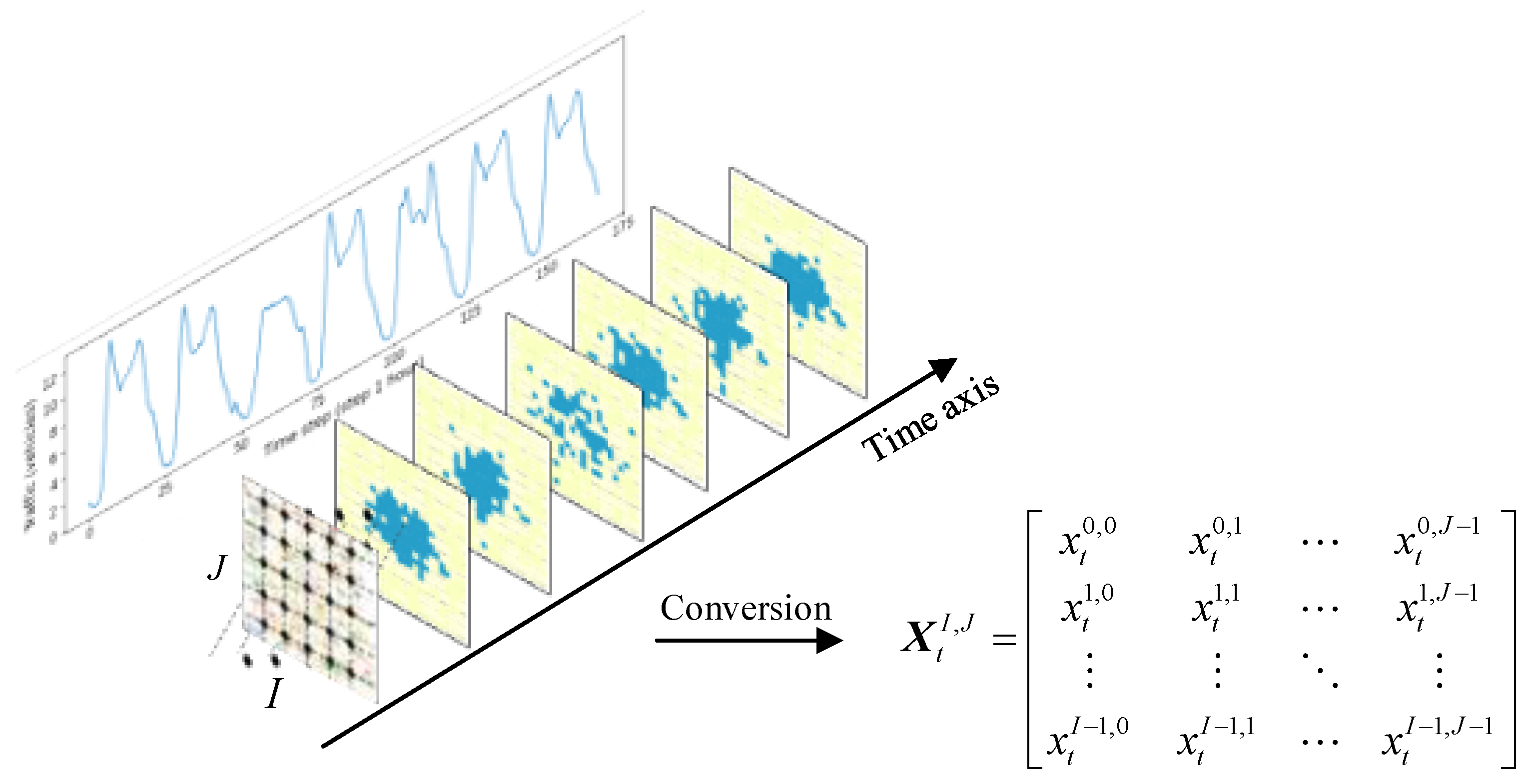
According to Atluri et al. [42], raster data is one of the most important data structures in the real world. By constantly observing spatial–temporal data and collecting data at a fixed place and time, we can see that the Euclidean structure data with equal position and spacing between intersections in Figure 1 is called raster data. To this end, we firstly divide the area of traffic data into raster areas with a dimension of I × J by latitude and longitude. Secondly, we record the traffic data of each location at a fixed time interval ∆t. The urban traffic data of the network area I × J is represented by Xt ∈ ℝI×J, and Xt is named as the traffic raster data; xt i,j represents the urban traffic data stored in the location (i, j) at time t.
3.2. Problem Definition
After conversion in Section 3.1, the traffic prediction problem is transformed into the given historical traffic raster data {Xt|t = 0, …, k} to predict the data Xk+∆t at a certain time interval k + ∆t, where k is the last time node for traffic raster data. There are three difficulties in this problem: firstly, how to evaluate the association between historical data; secondly, how to extract the dynamic spatial-temporal features of urban road network; and finally, how to select the model parameters.
3.3. Long-Term and Short-Term Characteristics of Traffic Data
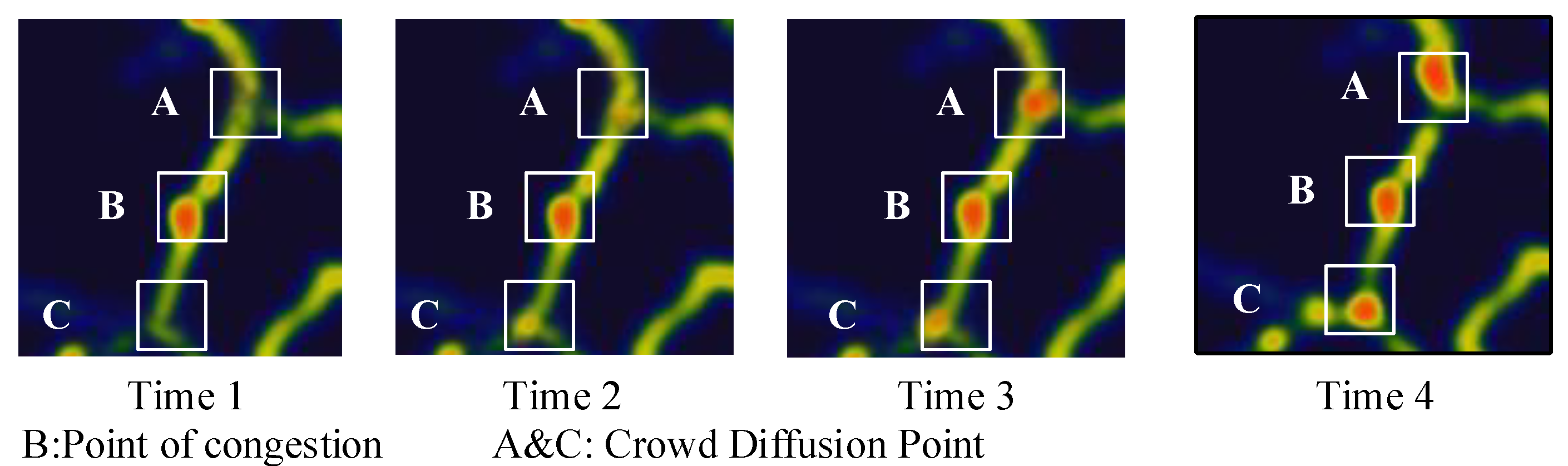
Traffic data include dynamic spatial characteristics and long-term temporal characteristics. Take the traffic congestion propagation shown in Figure 2 as an example, there are three points, i.e., A, B and C, in which point B is the place where congestion occurs, and points A and C are the places where congestion is transmitted. This phenomenon of congestion transmission reflects the dynamic spatial characteristics of traffic data. At the same time, this congestion phenomenon only occurs in a certain period of time. In a long time, the traffic data at points A, B and C have periodic characteristics, so the traffic data have significant long-term temporal characteristics.
4. Methodology
In this section, we will first present the architecture of the spatial–temporal residual model. Then, the structure of the spatial–temporal 3D residual correlation network will be introduced.
4.1. Basic Architecture of Spatial–Temporal Residual Model
Section 3 shows that traffic data has significant spatial–temporal characteristics. Considering only one of these characteristics will result in poor prediction model accuracy. Based on the selection of convolution kernel dimensions, 2D and 3D spatial–temporal residual models have been proposed. The spatial–temporal residual model extracts traffic characteristics by combining convolution operation and residual units; the structure of typical ST-ResNet is shown in Figure 3.
4.2. Spatial–Temporal 3D Residual Correlation Network
4.2.1. Basic Structure of Spatial–Temporal 3D Residual Correlation Network
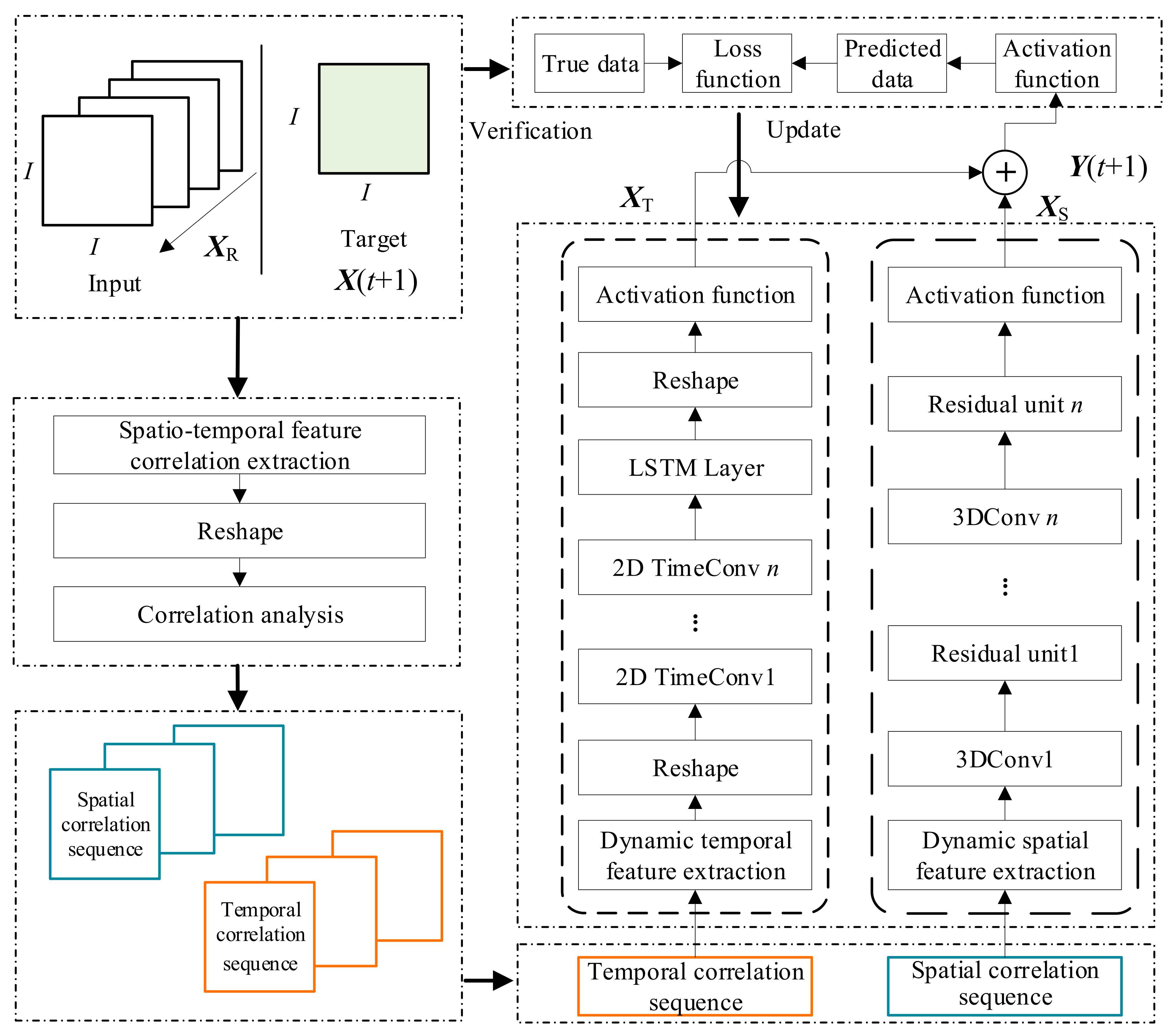
As described in Section 1, to extract the dynamic evolution characteristics of traffic information, we propose a spatial–temporal 3D residual correlation network (ST-3DRCN) for urban traffic status prediction. ST-3DRCN consists of a spatial–temporal correlation feature extraction component, and a dynamic spatial and temporal feature extraction component. First, we apply the Pearson correlation coefficient method to extract high symmetric correlation between historical traffic data. Then, a dynamic spatial feature extraction component is constructed by using 3D convolution combined with residual units to extract the dynamic spatial features. After that, the “2D temporal convolution” block is proposed with LSTM to clarify the contributions of the dynamic temporal features. Finally, the dynamic spatial and temporal features are weighted out, and the final predicted value is obtained. The structure of the ST-3DRCN is shown in Figure 4.
4.2.2. Spatial–Temporal Correlation Feature Extraction Component
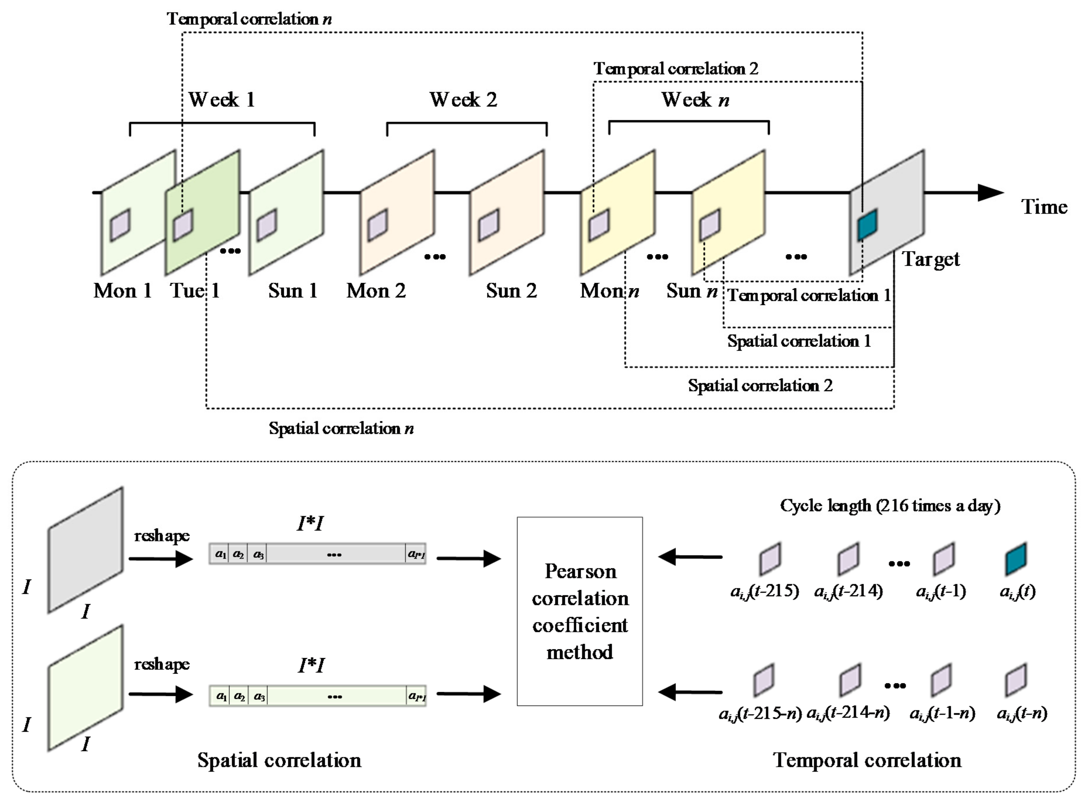
This paper mainly uses historical traffic raster data to predict the traffic raster data of a future node at a certain time. The historical traffic raster data of different time nodes have some symmetric correlation, as shown in Figure 5.
In order to calculate the symmetric correlation between traffic raster data, the Pearson correlation coefficient method is used to analyze the correlation between data [43]. The Pearson correlation coefficient formula is:
where xi and yi (i = 1, …, n) are the target traffic raster data and the traffic raster data to be compared, respectively; and σx and σy are the sample population standard deviation of the target traffic raster data and the traffic raster data to be compared, respectively. We divide the original traffic raster data into spatial and temporal series based on the Pearson correlation coefficient method.
4.2.3. Dynamic Spatial Feature Extraction Component
We use 3D convolution and residual units to construct a dynamic spatial feature extraction component, as shown in Figure 6. Take the traffic raster data dimension I × I for example. Selecting M × M traffic raster data from spatial sequence to construct 3D traffic raster data with M × I × I dimension, convolution kernel dimension is set to w × h × j, step is set to s, and no pooling is done. The dynamic spatial feature extraction component 3D convolution operation is defined as:
where Xsl−1 and Xsl are the input and output of the l-th layer of the dynamic spatial feature extraction component 3D convolution operation, respectively, Wsl is the 3D convolution kernel, bsl is the bias term of the l-th 3D convolution layer, LS is the number of layers that the dynamic spatial feature extraction component 3D convolution operation needs to convolute, and fAF is the activation function.
To avoid the problem of model precision degradation due to the large number of convolution layers, we introduce residual units to improve the sensitivity, as shown in Figure 6. The output Xsl of the dynamic spatial feature extraction component 3D convolution operation is input to the residual unit. The residual operation of the dynamic spatial feature extraction component is defined as:
where ZRl−1 and ZRl are the input and output of the l-th residual unit, respectively, θRl is the set of learnable parameters in the l-th residual unit, FR is the residual mapping of the dynamic spatial feature extraction component, and LR is the number of residual layers required for dynamic spatial feature. After the output of the dynamic spatial feature extraction component is processed by residual operation, the dynamic spatial feature output XS is obtained.
4.2.4. Dynamic Temporal Feature Extraction Component
In addition to extracting the dynamic spatial feature from urban traffic data, we also need to extract the dynamic temporal feature. In this component, As shown in Figure 7, we designed a new architecture unit of the “2D time convolution” block to extract dynamic temporal features. The 2D temporal convolution operation is similar to the 3D convolution operation formula. The difference is that the 2D temporal convolution operation converts the dimension of M traffic raster data in the time series from (M, I, I) to (M, I × I), and the convolution kernel with design dimension (M, 1) is transformed to extract dynamic temporal characteristics with dimension (1, I × I).
To ensure that long-term temporal features are extracted from the dynamic temporal evolution of the traffic raster data, we input the traffic raster data after extracting the dynamic temporal into the LSTM network to maintain the long-term time characteristics. The overall formula for dynamic temporal feature extraction components is defined as:
where x(t − 1) and x(t) are the input and output of the 2D temporal convolution operation, respectively. h(t) and h(t − 1) are the unit outputs of the LSTM at the current and last moment, respectively. s(t) and s(t − 1) are the cell states of the LSTM at the current and last moment, respectively. g(t) is the cell state used to describe the current input to LSTM. f(t) is the forgetting gate, i(t) is the input gate, and o(t) is the output gate. W and b are the weight and offset terms of each unit, respectively. σ is the activation function, and fReLu is ReLu function. Finally, we get the output XT of the dynamic time feature extraction component.
4.2.5. Fusion
We adopt a parameter matrix fusion method to perform weighted fusion of the dynamic spatial feature output XS, and dynamic temporal feature output XT. The weight value is dynamically adjusted according to training. The formula is:
4.2.6. Loss Function
The index mean square error (MSE) is used as the loss function to evaluate the errors of real value and predicted value in model training.
where XTr and XPr are the real value and predicted value respectively, and n is the total number of samples.
5. Experiments
In this section, two traffic datasets will be applied in our experiment to evaluate the performance of ST-3DRCN. The experimental parameters will be set as follows.
5.1. Datasets
We select two typical data to validate the predictive performance of different models, TaxiCD (Urban road data) and PEMS-BAY (Expressway data).
- (a)
- TaxiCD: The experimental data comes from GPS data of taxis in Chengdu, China from 3 August 2014 to 20 August 2014. The data is of a real road from 6 am to 12 pm every day. Data details are shown in Table 1. We convert taxi data into traffic raster data with 36 × 36 dimensions based on the information in Table 1. In this article, a number of taxis are used in the raster to represent urban traffic status. TaxiCD is a typical Euclidean structure data set, which is mainly used to compare the prediction performance of models processing Euclidean data.
- (b)
- PEMS-BAY: PEMS-BAY data from the California Department of Transportation recorded five-month data from 325 sensors (1 January 2017~31 May 2017) at five-minute intervals. PEMS-BAY is a typical non-Euclidean data used to evaluate the predictive performance of models suitable for non-Euclidean data.
Figure 8 shows the rasterization of the map of Chengdu. Point A represents a raster involved in road links, and point B represents a roadless raster.
5.2. Hyperparameter
Our model is developed by using Pytorch-GPU and parameter iteration in model training through the Adam optimization algorithm. The training step is set at 0.0001, the number of batches is set at 20, and the maximum number of iterations is set at 800. The other parameters of our model are shown in Table 2.
5.3. Traffic Status Transformation and Standardization
In order to better show the traffic status, we will protocol the traffic raster data. According to the number of automobiles counted by the traffic raster data, we divide into six traffic states, one for smooth traffic and six for heavy congestion. After the traffic status data is generated, we need to standardize the traffic raster data to reduce the influence of different dimensions between the data, and the calculation formula is as follows:
where is the n-th data in the traffic raster data, is the average value of all traffic raster data, and is the standard deviation of the overall traffic raster data.
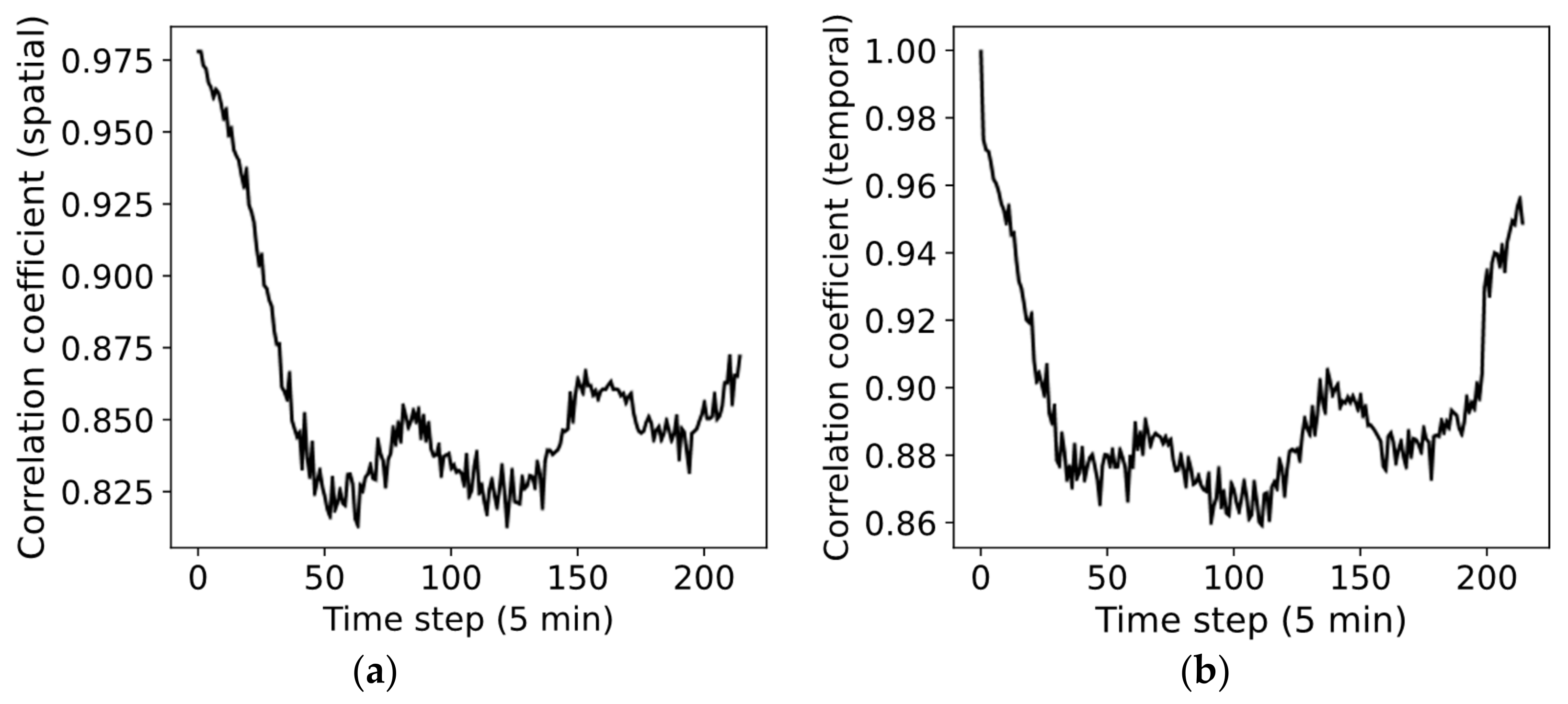
5.4. Spatial–Temporal Correlation Feature Extraction
To ensure a strong symmetric correlation between the input data, the Section 4.2.2 method is used to extract the spatial–temporal correlation characteristics of the raster data. Taking x0,17 data of TaxiCD as an example, the spatial–temporal correlation is shown in Figure 9. Figure 9a,b show the spatial–temporal correlation of traffic data in a day. The accuracy of the model can be improved by using time nodes that are highly associated with them.
5.5. Baseline Models
To better reflect the prediction accuracy of the proposed model, we use the following five baseline models as comparisons to verify the prediction effect.
- LSTM: Long short-term memory network, as an improved RNN, effectively reduces the gradient disappearance and gradient explosion during RNN training. LSTM is often used to extract the temporal characteristics of traffic information.
- CNN: Convolution neural network or 2D-CNN uses a 2D convolution kernel to extract spatial features of two-dimensional data.
- 3D-CNN: Unlike 2D-CNN, 3D-CNN uses a 3D convolution kernel to extract spatial features of 3D data. Compared with 2D-CNN, it is easier to find the dynamic characteristics.
- ST-ResNet: The spatial–temporal residual network is a deep neural network used to extract spatial–temporal features.
- ST-3DNet: Deep spatial–temporal 3D convolutional neural network uses 3D convolution combined with residual units to extract spatial and temporal features of traffic information.
- ST-GCN: Spatial–temporal graph convolutional network, ST-GCN considers time series as one of the factors on the basis of traditional GCN.
- DGLSTNet: Dynamic global-local spatial–temporal network, which consists of multiple spatial–temporal modules and focuses on local and global information of traffic data on the basis of ST-GCN.
5.6. Evaluating Indicator
In order to scientifically evaluate the prediction effects of different models, we use root mean square error (RMSE) and mean absolute error (MAE) to compare the prediction results of the models. The two formulas are as follows:
where yi is the true value of traffic data, is the traffic data predicted by the model, and m is the number of samples.
6. Results
The experiments will be carried out according to the steps outlined in the above sections. In order to verify the superiority of the proposed ST-3DRCN model, the results from the proposed model will be compared with LSTM, CNN, 3D-CNN, ST-ResNet, ST-GCN, DGLSTNet and ST-3DNet. The Euclidean and non-Euclidean traffic data will be analyzed respectively. The possible network topologies to be employed in ST-3DRCN and its influence on the results will also be investigated.
6.1. The Global-Local Predictions Based on the ST-3DRCN
After the initialization of our model, we use the training set to train, and use the test set of TaxiCD to verify the prediction effects. The ST-3DRCN prediction results of local positions are shown in Figure 10. The prediction results of the training set and the test set are before and after node 431, respectively.
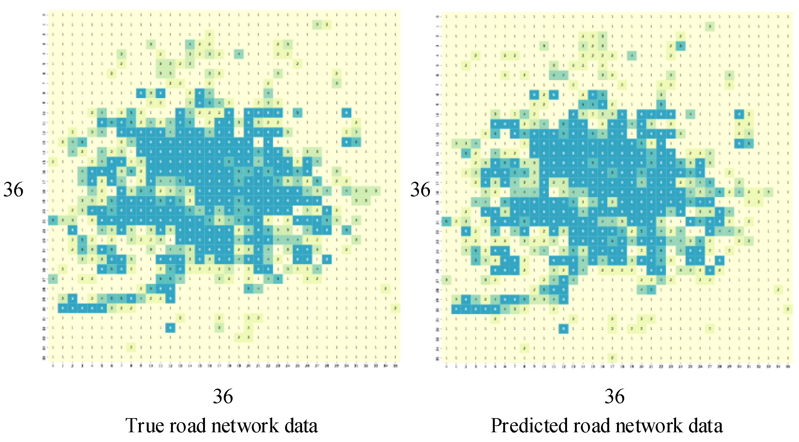
Meanwhile, we also verify the prediction performance of the model to the global status; Figure 11 shows a comparison between the true value and the predicted value of the global traffic status at a certain time. The color depth in the graph represents the number of vehicles. The deeper the color, the larger the number of vehicles.
6.2. Comparison with Five Classical Baseline Models
6.2.1. Settings of Baseline Models
In order to verify the prediction performance of ST-3DNet on Euclidean urban road network data, we evaluate our proposed model by comparing the results of five classical baseline models. Some parameters of all models are set uniformly to verify the prediction effect between models fairly. The specific parameter settings are shown in Table 3.
6.2.2. Comparison Results with Five Classical Baseline Models
We used TaxiCD to train and test six models. Table 4 shows the accuracy comparison between our model and the baseline model with RMSE and Mae as evaluation indicators. Based on LSTM, CNN, 3D-CNN, ST-ResNet and ST-3DNet, the prediction accuracy of the proposed model is improved by 21.4%, 21.3%, 11.7%, 10.8% and 2.3%, respectively, with RMSE as the evaluation index.
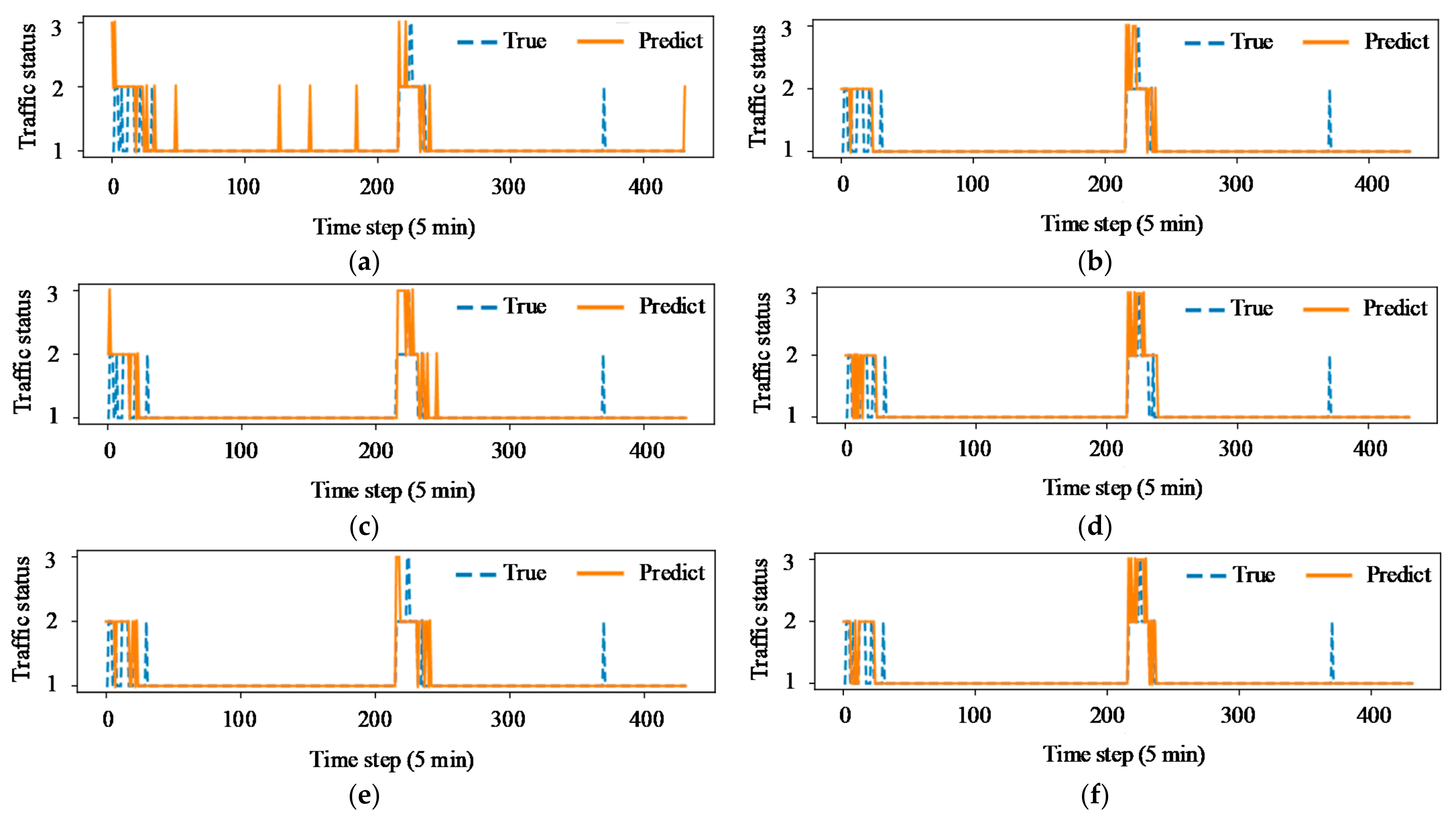
In the city traffic management, we need to understand the traffic status of a section or a point, so we need to compare the prediction effect of different models on a point in the raster data. Figure 12 shows the effect of different models on traffic status prediction at the same point.
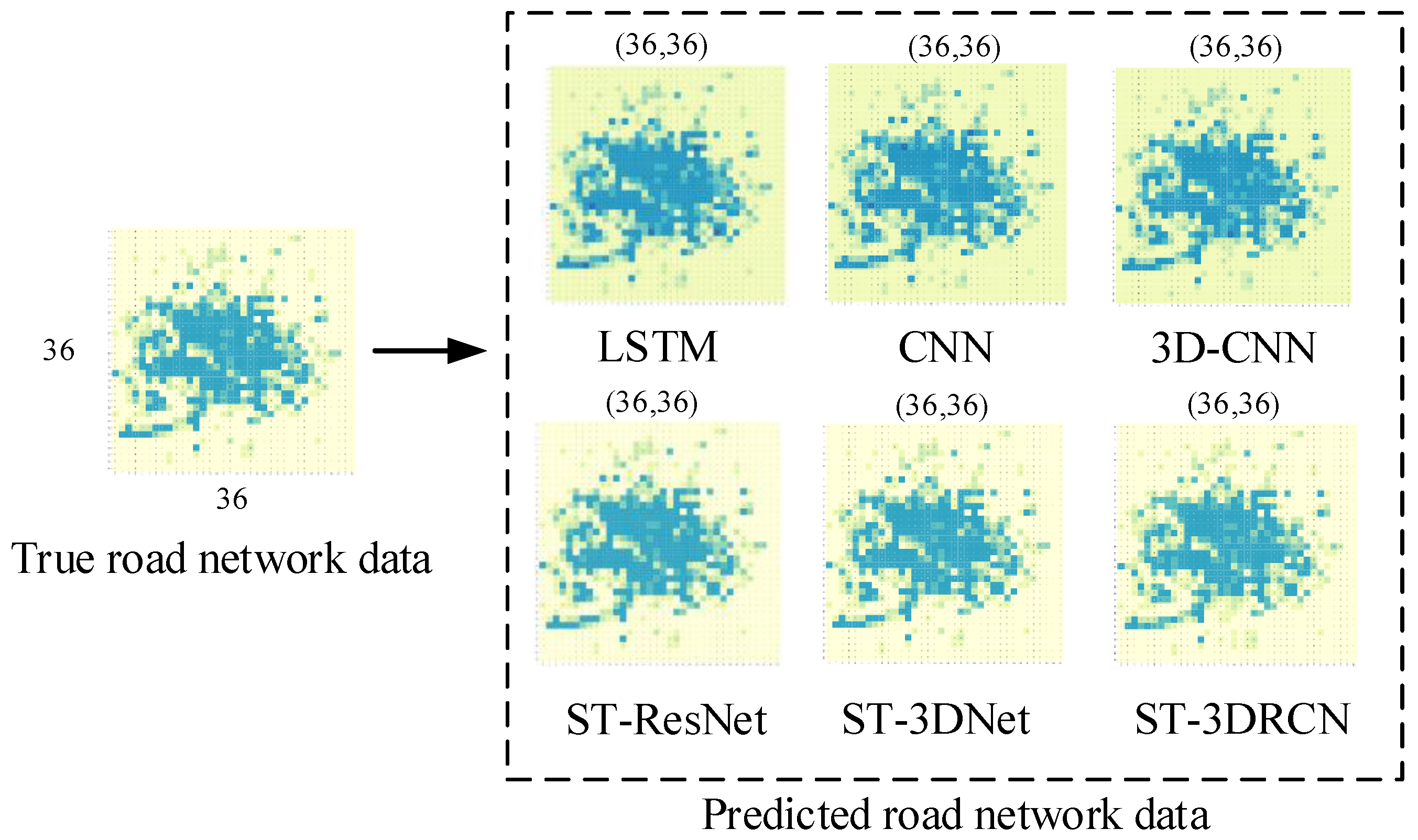
In order to verify the prediction effect of all models on global traffic conditions, we also need to predict all areas of urban road network. Figure 13 shows the prediction effects of different models on the global region. To compare the similarity between predicted and real data from different models, we use the Pearson correlation coefficient method to list the similarity of each group of data, as shown in Figure 14.
We choose different time intervals to verify the multi-step prediction ability of the model. The multi-step prediction ability determines the effect of the model on the extraction of long-term features of traffic data. Referring to the work of [8], the selection of time span is random. For the convenience of statistics, the time interval ranges from 5 min to 60 min. Figure 15a and Figure 16b show the short-term (0–30 min) prediction accuracy of different models, respectively. Figure 16a,b show the long-term (30–60 min) of different models, respectively.
Training time is also one of the indicators of the evaluation model. The shorter the training time of a model is, the stronger the application ability of the model in actual production is. The number of iterations for all models is set to 800, and the loss iteration is shown in Figure 17. It can be seen from the figure that ST-3DRCN has a faster convergence speed.
6.3. Comparison with Two Typical Models Dealing with Non-Euclidean Data
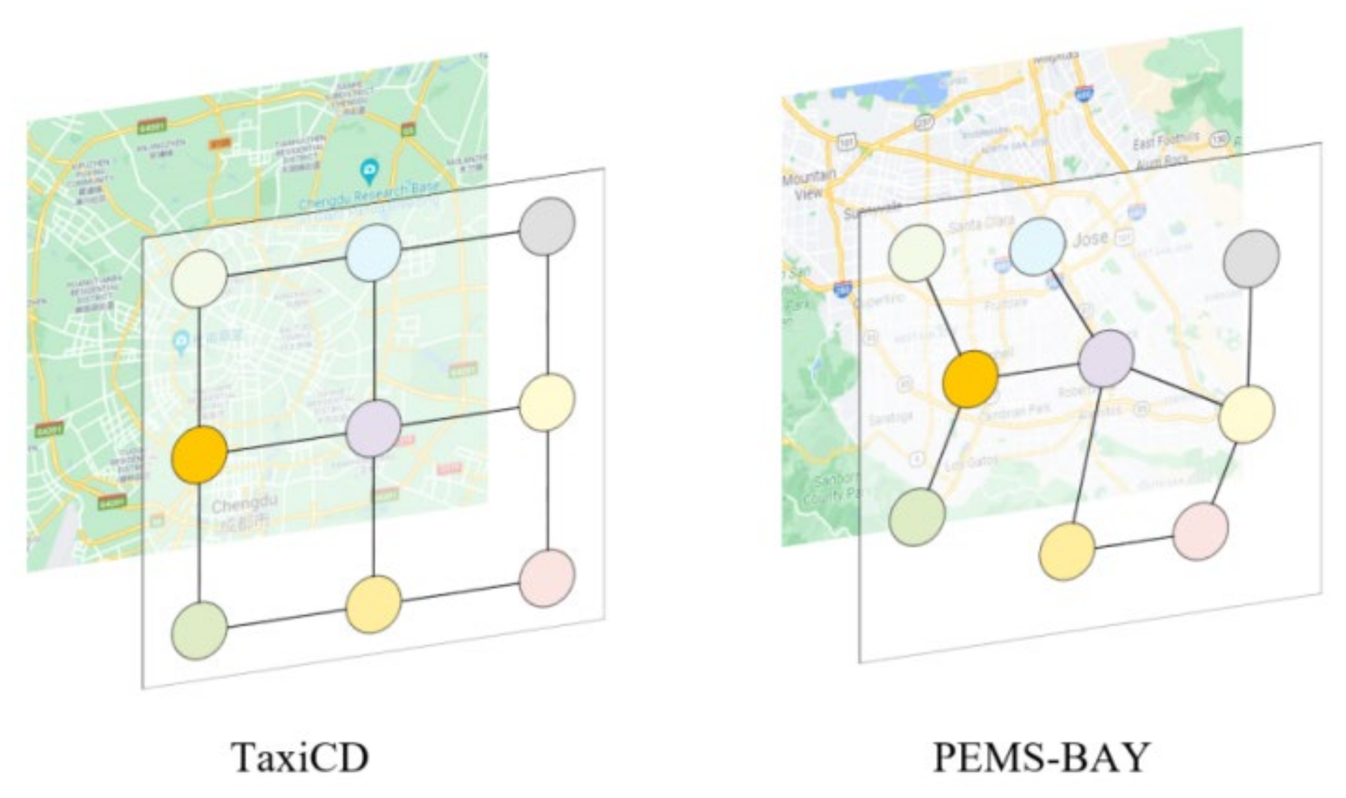
In order to verify the prediction performance of our proposed model for non-Euclidean data, we use two typical models, ST-GCN and DGLSTNet, as baseline models to compare the prediction performance. We used data of TaxiCD and PEMS-BAY to train and test all models. The structures of TaxiCD and PEMS-BAY are shown in Figure 18. Based on the two structures, we can get the adjacency matrix.
The prediction results of models are shown in the Table 5. On the TaxiCD dataset, the prediction performance of ST-3DRCN is the best; on the PEMS-BAY dataset, DGLSTNet has the best prediction performance. For Euclidean and non-Euclidean traffic data, ST-3DRCN and DGLSTNet have the best prediction accuracy, respectively. Taking RMSE as the evaluation index, the prediction accuracy of ST-3DRCN on the TaxiCD dataset is 4.7% and 3.6% higher than that of ST-GCN and DGLSTNet, respectively.
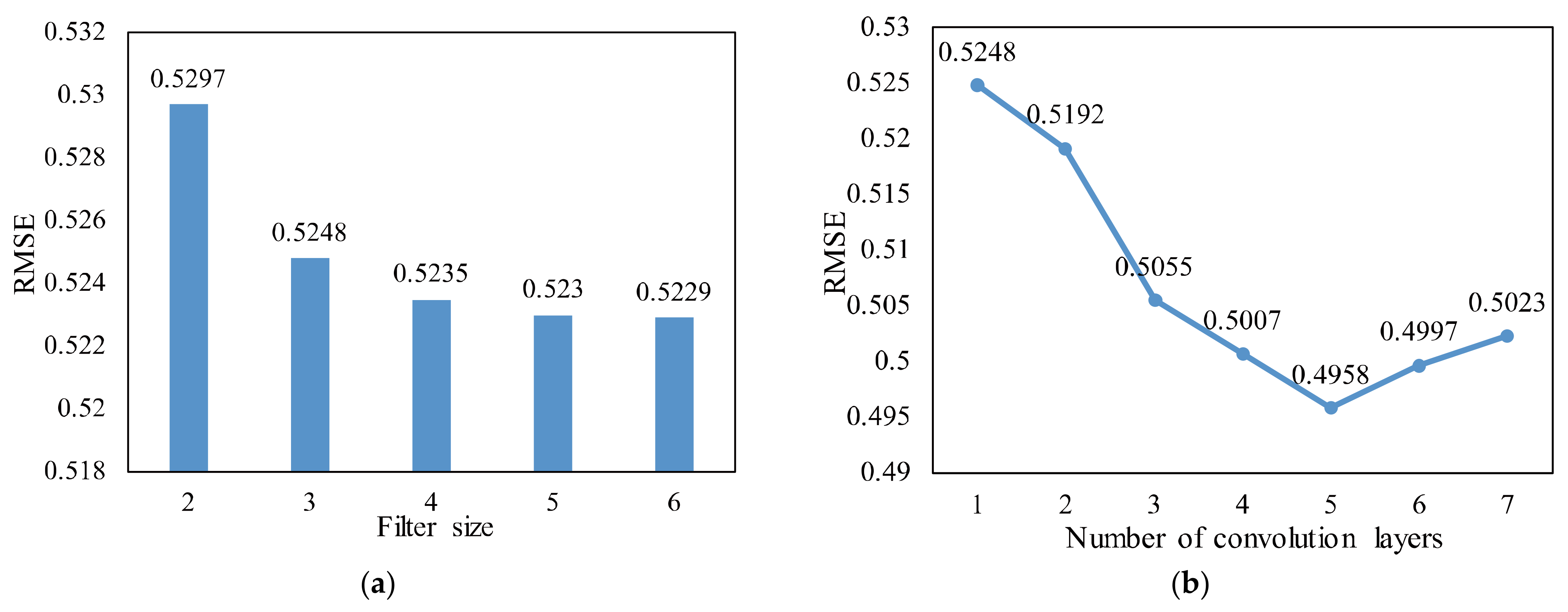
6.4. Network Configuration of the ST-3DRCN
In order to study the impact of different network structures on the model, taking RMSE as the evaluation index and TaxiCD as the data set, we established two groups of control experiments. Figure 19a shows the prediction accuracy of the proposed model when the convolution layer is 1 and the filter size changes from 2 × 2 to 6 × 6. Considering that the larger the size of convolution kernel, the greater the computational cost of the model, we set the size of filter size to 3 × 3. Figure 19b shows the accuracy of the proposed model when the filter size is 3 × 3 and the number of convolution layers increases from 1 to 7. Experiments show that the optimal parameters of the model on TaxiCD dataset are: the filter size set to 3 × 3 and the number of convolution layers set to 5.
6.5. Discussion
From the numerical results in Section 6.1, Section 6.2, Section 6.3 and Section 6.4, we see that our proposed ST-3DRCN model shows a significant improvement on the prediction accuracy. Meanwhile, the effectiveness of the proposed method is further proved by comparison with other classical models. These models include LSTM, CNN, 3D-CNN, ST-ResNet, ST-3DNet, ST-GCN, and DGLSTNet.
In particular, ST-3DRCN shows excellent performance in extracting dynamic spatial–temporal features from traffic data. The results of the experiment show that LSTM is a time series-based prediction model, which has a strong ability to capture the temporal characteristics of traffic data, but a poor ability to capture the spatial characteristics. CNN, as a traditional prediction model for mining spatial characteristics, is difficult to capture the temporal characteristics. 3D-CNN enhances the capture of dynamic traffic characteristics based on CNN. ST-ResNet and ST-3DNet do not filter the time series when dealing with traffic data of urban road network. They are easy to capture time series with low correlation and ignore the long-term time characteristics when capturing small changes.
ST-GCN and DGLSTNet have excellent prediction performance in non-Euclidean traffic data, but ignore the dynamic spatial correlation and long-term time characteristics of traffic data, resulting in the above two models not performing as well as ST-3DRCN in Euclidean traffic data processing.
At the same time, it should be pointed out that choosing the appropriate network parameters is very important to improve the prediction performance of ST-3DRCN.
In summary, through the experimental comparison of the above sections, it is found that the ST-3D RCN model proposed in this paper has better prediction performance in an urban environment. Compared with other baseline models, ST-3DRCN not only extracts dynamic spatial features effectively, but also has the ability to extract long-term temporal features. As shown in Figure 20, taking the root mean square error (RMSE) as the evaluation index, the prediction accuracy of ST-3DRCN on TaxiCD dataset is 21.4%, 21.3%, 11.7%, 10.8%, 4.7%, 3.6% and 2.3% higher than LSTM, CNN, 3D-CNN, ST-ResNet, ST-GCN, DGLSTNet and ST-3DNet, respectively. Therefore, the ST-3D RCN model proposed in this paper is more suitable for urban road network traffic data prediction.
7. Conclusions
In this paper, we propose a novel spatial–temporal 3D residual correlation network (ST-3DRCN) for predicting urban traffic status. ST-3DRCN introduces the Pearson correlation coefficient method to obtain the spatial and temporal symmetric correlation series. A dynamic spatial feature extraction component is constructed by using 3D convolution and residual units, and the component is used to extract the dynamic spatial features. A novel “2D temporal convolution” block is proposed to extract the dynamic temporal features. We used TaxiCD and PEMS-BAY data sets to verify the prediction accuracy of the proposed ST-3DRCN model. The experimental results show that the prediction accuracy of the proposed model is improved by 10.8% on average, compared with the baseline models such as LSTM, CNN, 3D-CNN, ST-ResNet, ST-GCN, DGLSTNet and ST-3DNet. Our next work will focus on the problem of reduced prediction accuracy due to model structure solidification.
Author Contributions
Conceptualization, Y.-X.B. and Q.S.; Methodology, Y.-X.B. and Y.C.; Writing—original draft preparation, Y.-X.B. and Q.-Q.S.; Project administration, Q.S., Q.-Q.S. and Y.C.; Funding acquisition, Q.S., Q.-Q.S. and Y.C.; Writing—review and editing, Q.S., Q.-Q.S. and Y.C.; Validation, Q.S., Q.-Q.S. and Y.C. All authors have read and agreed to the published version of the manuscript.
Funding
This research was funded by the National Natural Science Foundation of China, grant number 61771265; the “333” Scientific Research Project of Jiangsu, grant number BRA2017475; the Qinglan Project of Jiangsu Province; the Nantong Science and Technology Program Project, grant numbers MS22021034 and JC2021198; the “226” Scientific Research Project of Nantong, grant number 131320633045.
Institutional Review Board Statement
Not applicable.
Informed Consent Statement
Not applicable.
Data Availability Statement
The data used to support the findings of this study are available from the last author upon request.
Acknowledgments
The authors would like to thank the editors for their help and the anonymous reviewers for their guidance so that the paper can be completed.
Conflicts of Interest
The authors declare that they have no conflict of interest in this work.
References
- Zhang, J.P.; Wang, F.Y.; Wang, K.F.; Lin, W.H.; Xu, X.; Chen, C. Data-driven intelligent transportation systems: A survey. IEEE Trans. Intell. Transp. 2011, 12, 1624–1639. [Google Scholar] [CrossRef]
- Basheer, S.; Srinivasan, K.K.; Sivanandan, R. Investigation of information quality and user response to real-time traffic information under heterogeneous traffic conditions. Transp. Dev. Econ. 2018, 4, 1–11. [Google Scholar] [CrossRef]
- Vlahogianni, E.I.; Karlaftis, M.G.; Golias, J.C. Short-term traffic forecasting: Where we are and where we’re going. Transport. Res. C-Emer. 2014, 43, 3–19. [Google Scholar] [CrossRef]
- Zhou, Y.; Wang, J.; Yang, H. Resilience of transportation systems: Concepts and comprehensive review. IEEE Trans. Intell. Transp. 2019, 20, 4262–4276. [Google Scholar] [CrossRef]
- Zhao, L.; Song, Y.J.; Zhang, C.; Liu, Y.; Wang, P.; Lin, T.; Deng, M.; Li, H.F. T-GCN: A temporal graph convolutional network for traffic prediction. IEEE Trans. Intell. Transp. 2019, 21, 3848–3858. [Google Scholar] [CrossRef] [Green Version]
- Zhang, W.; Yu, Y.; Qi, Y.; Shu, F.; Wang, Y. Short-term traffic flow prediction based on spatio-temporal analysis and CNN deep learning. Transp. A 2019, 15, 1688–1711. [Google Scholar] [CrossRef]
- Zhang, J.B.; Zheng, Y.; Qi, D.K.; Li, R.Y.; Yi, X.W.; Li, T.R. Predicting citywide crowd flows using deep spatio-temporal residual networks. Artif. Intell. 2018, 259, 147–166. [Google Scholar] [CrossRef] [Green Version]
- Guo, S.N.; Lin, Y.F.; Li, S.J.; Chen, Z.M.; Wan, H.Y. Deep spatial–temporal 3D convolutional neural networks for traffic data forecasting. IEEE Trans. Intell. Transp. 2019, 20, 3913–3926. [Google Scholar] [CrossRef]
- Nagy, A.M.; Simon, V. Survey on traffic prediction in smart cities. Pervasive Mob. Comput. 2018, 50, 148–163. [Google Scholar] [CrossRef]
- Lana, I.; Del Ser, J.; Velez, M.; Vlahogianni, E.I. Road traffic forecasting: Recent advances and new challenges. IEEE Intel. Transp. Syst. 2018, 10, 93–109. [Google Scholar] [CrossRef]
- Jha, K.; Sinha, N.; Arkatkar, S.S.; Sarkar, A.K. A comparative study on application of time series analysis for traffic forecasting in India: Prospects and limitations. Curr. Sci. 2016, 110, 373–384. [Google Scholar] [CrossRef]
- Guo, F.; Polak, J.W.; Krishnan, R. Predictor fusion for short-term traffic forecasting. Transport. Res. C-Emer. 2018, 92, 90–100. [Google Scholar] [CrossRef]
- Lippi, M.; Bertini, M.; Frasconi, P. Short-term traffic flow forecasting: An experimental comparison of time-series analysis and supervised learning. IEEE Trans. Intell. Transp. 2013, 14, 871–882. [Google Scholar] [CrossRef]
- Kang, C.; Zhang, Z. Application of LSTM in short-term traffic flow prediction. In Proceedings of the 2020 IEEE 5th International Conference on Intelligent Transportation Engineering, Beijing, China, 11–13 September 2020. [Google Scholar]
- Hamed, M.M.; Al-Masaeid, H.R.; Said, Z.M.B. Short-term prediction of traffic volume in urban arterials. J. Transp. Eng. 1995, 121, 249–254. [Google Scholar] [CrossRef]
- Kumar, S.V.; Vanajakshi, L. Short-term traffic flow prediction using seasonal ARIMA model with limited input data. Eur. Transp. Res. Rev. 2015, 7, 1–9. [Google Scholar] [CrossRef] [Green Version]
- Kumar, S.V. Traffic flow prediction using Kalman filtering technique. Procedia. Eng. 2017, 187, 582–587. [Google Scholar] [CrossRef]
- Chan, K.Y.; Dillon, T.S.; Singh, J.; Chang, E. Neural-network-based models for short-term traffic flow forecasting using a hybrid exponential smoothing and Levenberg–Marquardt algorithm. IEEE. Intel. Transp. Syst. 2011, 13, 644–654. [Google Scholar] [CrossRef]
- Shen, Q.Q.; Cao, Y.; Yao, L.Q.; Zhu, Z.K. An optimized discrete grey multi-variable convolution model and its applications. Comput. Appl. Math. 2021, 40, 1–26. [Google Scholar] [CrossRef]
- Feng, X.; Ling, X.; Zheng, H.; Chen, Z.; Xu, Y. Adaptive multi-kernel SVM with spatial–temporal correlation for short-term traffic flow prediction. IEEE Trans. Intell. Transp. 2019, 20, 2001–2013. [Google Scholar] [CrossRef]
- Tan, M.; LI, Y.; Xu, J. A hybrid ARIMA and SVM model for traffic flow prediction based on wavelet denoising. J. Highw. Transp. Res. Dev. 2009, 7, 126–133. [Google Scholar]
- Tang, J.; Chen, X.; Hu, Z.; Zong, F.; Han, C.; Li, L. Traffic flow prediction based on combination of support vector machine and data denoising schemes. Phys. A 2019, 534, 1–19. [Google Scholar] [CrossRef]
- Li, Z.; Jiang, S.; Li, L.; Li, Y. Building sparse models for traffic flow prediction: An empirical comparison between statistical heuristics and geometric heuristics for Bayesian network approaches. Transp. B 2019, 7, 107–123. [Google Scholar] [CrossRef]
- Liu, Z.; Du, W.; Yan, D.M.; Chai, G.; Guo, J.H. Short-term traffic flow forecasting based on combination of k-nearest neighbor and support vector regression. J. Highw. Transp. Res. Dev. 2018, 12, 89–96. [Google Scholar] [CrossRef]
- Lv, Y.; Duan, Y.; Kang, W.; Li, Z.; Wang, F.Y. Traffic flow prediction with big data: A deep learning approach. IEEE Trans. Intell. Transp. 2014, 16, 865–873. [Google Scholar] [CrossRef]
- Polson, N.G.; Sokolov, V.O. Deep learning for short-term traffic flow prediction. Transport. Res. C-Emer. 2017, 79, 1–17. [Google Scholar] [CrossRef] [Green Version]
- Huang, W.; Song, G.; Hong, H.; Xie, K. Deep architecture for traffic flow prediction: Deep belief networks with multitask learning. IEEE Trans. Intell. Transp. 2014, 15, 2191–2201. [Google Scholar] [CrossRef]
- Abdulhai, B.; Porwal, H.; Recker, W. Short-term traffic flow prediction using neuro-genetic algorithms. J. Intell. Transport. Syst. 2002, 7, 3–41. [Google Scholar]
- Hu, W.; Yan, L.; Liu, K.; Wang, H. A short-term traffic flow forecasting method based on the hybrid PSO-SVR. Neural Process. Lett. 2016, 43, 155–172. [Google Scholar] [CrossRef]
- Dai, S.; Niu, D.; Han, Y. Forecasting of power grid investment in China based on support vector machine optimized by differential evolution algorithm and grey wolf optimization algorithm. Appl. Sci. 2018, 8, 636. [Google Scholar] [CrossRef] [Green Version]
- Lee, S.; Kim, H.; Lieu, Q.X.; Lee, J. CNN-based image recognition for topology optimization. Knowl.-Based Syst. 2020, 198, 1–14. [Google Scholar] [CrossRef]
- Ma, X.; Dai, Z.; He, Z.; Ma, J.; Wang, Y.; Wang, Y. Learning traffic as images: A deep convolutional neural network for large-scale transportation network speed prediction. Sensors 2017, 17, 818. [Google Scholar] [CrossRef] [PubMed] [Green Version]
- Li, Y.; Zhu, Z.; Kong, D.; Han, H.; Zhao, Y. EA-LSTM: Evolutionary attention-based LSTM for time series prediction. Knowl.-Based Syst. 2019, 181, 1–9. [Google Scholar] [CrossRef]
- Liu, Y.; James, J.Q.; Kang, J.; Niyato, D.; Zhang, S. Privacy-preserving traffic flow prediction: A federated learning approach. IEEE Int. Things 2020, 7, 7751–7763. [Google Scholar] [CrossRef]
- Yu, B.; Yin, H.; Zhu, Z. Spatio-temporal graph convolutional networks: A deep learning framework for traffic forecasting. arXiv 2017, arXiv:1709.04875. [Google Scholar]
- Feng, D.; Wu, Z.; Zhang, J.; Wu, Z. Dynamic global-local spatial-temporal network for traffic speed prediction. IEEE Access 2020, 8, 209296–209307. [Google Scholar] [CrossRef]
- Xingjian, S.H.I.; Chen, Z.; Wang, H.; Yeung, D.Y.; Wong, W.K.; Woo, W.C. Convolutional LSTM network: A machine learning approach for precipitation nowcasting. Adv. Neural Inf. Process. Syst. 2015, 28, 802–810. [Google Scholar]
- He, K.; Zhang, X.; Ren, S.; Sun, J. Deep residual learning for image recognition. In Proceedings of the 2016 IEEE Conference on Computer Vision and Pattern Recognition, Las Vegas, NV, USA, 26 June–1 July 2016. [Google Scholar]
- Ren, Y.; Zhao, D.; Luo, D.; Ma, H.; Duan, P. Global-local temporal convolutional network for traffic flow prediction. IEEE Trans. Intell. Transp. 2020, 10, 1–7. [Google Scholar] [CrossRef]
- Guo, G.; Zhang, T. A residual spatio-temporal architecture for travel demand forecasting. Transport. Res. C-Emer. 2020, 115, 1–12. [Google Scholar] [CrossRef]
- Zheng, C.; Fan, X.; Wen, C.; Chen, L.; Wang, C.; Li, J. Deepstd: Mining spatio-temporal disturbances of multiple context factors for citywide traffic flow prediction. IEEE Trans. Intell. Transp. 2019, 21, 3744–3755. [Google Scholar] [CrossRef]
- Atluri, G.; Karpatne, A.; Kumar, V. Spatial-temporal data mining: A survey of problems and methods. ACM Comput. Surv. 2018, 51, 1–41. [Google Scholar] [CrossRef]
- Benesty, J.; Chen, J.; Huang, Y.; Cohen, I. Pearson Correlation Coefficient; Springer: Berlin/Heidelberg, Germany, 2009; pp. 1–4. [Google Scholar]
Figure 1.
Traffic raster data.

Figure 2.
The spread of traffic congestion.

Figure 3.
Structure of typical ST-ResNet.

Figure 4.
Structure of the ST-3DRCN.

Figure 5.
Correlation of traffic raster data.

Figure 6.
Dynamic spatial feature extraction.

Figure 7.
Dynamic temporal feature extraction.

Figure 8.
The rasterization of the map of Chengdu.

Figure 9.
The rasterization of the map of Chengdu; (a) spatial correlation, (b) temporal correlation.
Figure 9.
The rasterization of the map of Chengdu; (a) spatial correlation, (b) temporal correlation.

Figure 10.
The local prediction effect of ST-3DRCN.

Figure 11.
The global prediction effect of ST-3DRCN.

Figure 12.
The effect of different models on traffic status prediction at the same point; (a) LSTM, (b) CNN, (c) 3D-CNN, (d) ST-ResNet, (e) ST-3DNet, (f) ST-3DRCN (our model).
Figure 12.
The effect of different models on traffic status prediction at the same point; (a) LSTM, (b) CNN, (c) 3D-CNN, (d) ST-ResNet, (e) ST-3DNet, (f) ST-3DRCN (our model).

Figure 13.
Prediction of regional traffic status by different models.

Figure 14.
Similarity of predicted and true values for different models.

Figure 15.
Comparison of short-term (0–30 min) prediction of five classical baseline models. (a) RMSE (0–30 min); (b) MAE (0–30 min).
Figure 15.
Comparison of short-term (0–30 min) prediction of five classical baseline models. (a) RMSE (0–30 min); (b) MAE (0–30 min).

Figure 16.
Comparison of long-term (30–60 min) prediction of five classical baseline models. (a) RMSE (30–60 min); (b) MAE (30–60 min).
Figure 16.
Comparison of long-term (30–60 min) prediction of five classical baseline models. (a) RMSE (30–60 min); (b) MAE (30–60 min).

Figure 17.
Comparison of the number of lost iterations of five classical baseline models.

Figure 18.
The structures of TaxiCD and PEMS-BAY.

Figure 19.
Impact of different network structures. (a) Effect of filter size on the performance of ST-3DRCN; (b) Effect of convolution layers on the performance of ST-3DRCN.
Figure 19.
Impact of different network structures. (a) Effect of filter size on the performance of ST-3DRCN; (b) Effect of convolution layers on the performance of ST-3DRCN.

Figure 20.
Proportion of ST-3DRCN prediction accuracy improvement based on baseline models.


Table 1.
Statistics of the traffic condition dataset.
| Dataset | TaxiCD | PEMS-BAY |
|---|---|---|
| Location | In Chengdu, China | In California, USA |
| Time span | 3 August 2014 to 20 August 2014 | 1 January 2017 to 31 May 2017 |
| Time interval | 5 min | 5 min |
| Raster size | (36, 36) | (36, 36) |
| Number of available time intervals | 3888 | 43,200 |
| Maximum Longitude and Latitude | (104.20591, 30.791764) | (−121.805543, 37.416413) |
| Minimum Longitude and Latitude | (103.944323, 30.583564) | (−122.078275, 37.249226) |
| Area | 576 square kilometers | 354 square kilometers |
Table 2.
Structure of the ST-3DRCN.
| Parameter | ST-3DRCN |
|---|---|
| Input dimension | [Batch_size, 36, 36] |
| Dimension of 2D Conv kernel | 1 × 3 |
| Step size of 2D Conv kernel | 1 |
| Dimension of 3D Conv kernel | 3 × 1 × 1 |
| Step size of 3D Conv kernel | 1 |
| Dimension of LSTM input layer | 1 × 1296 |
| Dimension of LSTM out layer | 1 × 1296 |
| Number of Residual units | 8 |
Table 3.
Parameter setting of five classical baseline models.
| Parameter | LSTM | CNN | 3D-CNN | ST-ResNet | ST-3DNet |
|---|---|---|---|---|---|
| Input dimension | (1, 1296) | (36, 36) | (2, 36, 36) | (36, 36) | (2, 36, 36) |
| Output dimension | (1, 1296) | (36, 36) | (36, 36) | (36, 36) | (36, 36) |
| Training times | 800 | 800 | 800 | 800 | 800 |
| Batchsize | 20 | 20 | 20 | 20 | 20 |
| Training step | 0.0001 | 0.0001 | 0.0001 | 0.0001 | 0.0001 |
| Time interval | 5 min | 5 min | 5 min | 5 min | 5 min |
Table 4.
Comparison of average accuracy.
| Model | TaxiCD | |
|---|---|---|
| RMSE | MAE | |
| LSTM | 0.6307 | 0.3217 |
| CNN | 0.6297 | 0.3167 |
| 3D-CNN | 0.5617 | 0.2804 |
| ST-ResNet | 0.5560 | 0.2792 |
| ST-3DNet | 0.5074 | 0.2430 |
| ST-3DRCN | 0.4958 | 0.2317 |
Table 5.
Comparison with the model considering global-local features (5 min).
| Model | TaxiCD | PEMS-BAY |
|---|---|---|
| RMSE (Average) | RMSE (Average) | |
| ST-GCN | 0.5203 | 2.2451 |
| DGLSTNet | 0.5147 | 2.1956 |
| ST-3DRCN | 0.4958 | 2.2132 |
Publisher’s Note: MDPI stays neutral with regard to jurisdictional claims in published maps and institutional affiliations. |
© 2021 by the authors. Licensee MDPI, Basel, Switzerland. This article is an open access article distributed under the terms and conditions of the Creative Commons Attribution (CC BY) license (https://creativecommons.org/licenses/by/4.0/).
Share and Cite
MDPI and ACS Style
Bao, Y.-X.; Shi, Q.; Shen, Q.-Q.; Cao, Y. Spatial-Temporal 3D Residual Correlation Network for Urban Traffic Status Prediction. Symmetry 2022, 14, 33. https://doi.org/10.3390/sym14010033
AMA Style
Bao Y-X, Shi Q, Shen Q-Q, Cao Y. Spatial-Temporal 3D Residual Correlation Network for Urban Traffic Status Prediction. Symmetry. 2022; 14(1):33. https://doi.org/10.3390/sym14010033
Chicago/Turabian StyleBao, Yin-Xin, Quan Shi, Qin-Qin Shen, and Yang Cao. 2022. "Spatial-Temporal 3D Residual Correlation Network for Urban Traffic Status Prediction" Symmetry 14, no. 1: 33. https://doi.org/10.3390/sym14010033
Note that from the first issue of 2016, this journal uses article numbers instead of page numbers. See further details here.