Incompatible Deformations in Additively Fabricated Solids: Discrete and Continuous Approaches

Abstract

The present paper is intended to show the close interrelationship between non-linear models of solids, produced with additive manufacturing, and models of solids with distributed defects. The common feature of these models is the incompatibility of local deformations. Meanwhile, in contrast with the conventional statement of the problems for solids with defects, the distribution for incompatible local deformations in additively created deformable body is not known a priori, and can be found from the solution of the specific evolutionary problem. The statement of the problem is related to the mechanical and physical peculiarities of the additive process. The specific character of incompatible deformations, evolved in additive manufactured solids, could be completely characterized within a differential-geometric approach by specific affine connection. This approach results in a global definition of the unstressed reference shape in non-Euclidean space. The paper is focused on such a formalism. One more common factor is the dataset which yields a full description of the response of a hyperelastic solid with distributed defects and a similar dataset for the additively manufactured one. In both cases, one can define a triple: elastic potential, gauged at stress-free state, and reference shape, and some specific field of incompatible relaxing distortion, related to the given stressed shape. Optionally, the last element of the triple may be replaced by some geometrical characteristics of the non-Euclidean reference shape, such as torsion, curvature, or, equivalently, as the density of defects. All the mentioned conformities are illustrated in the paper with a non-linear problem for a hyperelastic hollow ball.

1. Introduction

Additive manufacturing technologies, which are often referred to as 3D printing, comprise a promising avenue in modern industrial world [1]. Particular branches that are of great importance are: laser sintering [2], stereolithography [3], and a generalization of the latter, namely polymer-based additive manufacturing [4]. Methods for mathematical modeling of materials, produced with additive technologies, have been intensively developed in last decades. This is related to the urgent need of forecasting and optimization of additively manufactured parts quality [5]. One can find the recent results concerning the problem of residual stresses prediction in [6], the challenge of matching the initial shape compensation, aimed at lowering of their intensity in [7], and optimization problems with account of various parameters of additive processes in [8,9,10]. Notably, special attention is paid to geometrical effect [11], which has significant influence on the internal stress distributions and should be taken into account in processes modeling and in matching the optimal control for them [12].

The major theoretical efforts involve advancing the theory of surface growth, based upon the basic principles, which had been formulated in the middle of previous century. In them, the conception of growing deformable body, that is the body, which is subjected to deformation and influx of additional material to its boundary during the same time, was introduced [13]. These ideas have subsequently been reflected in various applications, even in astrophysical problems [14]. The theory of growing solids has greatly advanced in the works of the Soviet school [15]. A detailed survey of the works prior to 1985 can be found in [16].

To date, the state of the art of the surface growth theory can be illustrated with results, obtained from several areas. One of them covers the modeling of 3D printed solids with specific features, related with controllable distribution of incompatible deformations. This new branch in technology was very aptly named as printing of non-Euclidean solids [17,18]. The general approach is based on the non-Euclidean geometry of the reference shape. This approach has been considerably developed in recent works [19,20,21]. Special attention is paid to non-linear theory of surface growth [22]. One can find the statement and model solutions for the evolutionary problem that relates the specificity of internal geometry with scenario of body fabrication in [23,24].

The primary ideas, that provide the backbone of the theory of surface growth, are related to the non-Euclidean mechanics of continua. The literature on this subject is very extensive. We just outline a few monographs [25,26,27] and papers [28,29], which are directly relevant to the present study. The same approach has been already proved to be very fruitful in mathematical theory of distributed defects. It had been decisively demonstrated in classical works [30,31], related to continuously distributed dislocations and disclinations, as well as in their modern generalizations [32,33], that are able to take into account more generic types like topological defects and extra matter [34,35].

The present paper is aimed to show close interrelationship between non-linear models of solids, produced with additive manufacturing and models of solids with continuously distributed defects. It could be seen as a continuation of [23], focused on interpretation of incompatibility, induced by additive manufacture process, in terms of distributed defects.

Body manifold. The body manifold (or more shortly, the body) $\mathfrak{B}$ is a smooth manifold that serves as an abstract descriptor for the collection of material particles, which together constitute a solid (basic definitions for smooth manifolds and the elements of calculus on them can be found in [36,37]). The applications of modern differential-geometric approach in continuum mechanics were firstly developed by W. Noll and C.-C. Wang in [38,39]. One can find the state of the art in regard to this approach in [26,28,29,33,35,40,41,42,43,44,45,46]). It is relevant to note here, that the body manifold does not contain information about the positions of material points in physical space. In the case when physical attributes of material points, such as mass, do not matter, the body manifold might be regarded as the collection of labels like a list of particle identifiers, commonly used in conventional analytical mechanics. The only difference being that the underlying set of the body manifold is infinite and its cardinality is equal to the cardinality of continuum. To indicate the abstract character of the elements of the body manifold we will denote them by Fraktur majuscules $\mathfrak{X},\mathfrak{Y},\mathfrak{Z},\cdots$ In the whole paper we assume that the dimension of body manifold is equal to 3.

Shapes. A body is not directly observable, nonetheless one can observe the regions which are occupied by material points that constitute the body. We believe that these regions can be regarded as submanifolds of some ambient smooth three-dimensional manifold $\mathcal{P}$. We will just call them shapes, while $\mathcal{P}$ will be referred to as physical space. The elements of $\mathcal{P}$ will be called places and denoted by Latin script minuscules $\mathcal{X},\mathcal{Y},\mathcal{Z},\cdots$ We also suppose that body $\mathfrak{B}$ and all its shapes are topologically isomorphic.

Configurations and deformations. The correspondence between the body and its shapes is given by a set of injective mappings $\varkappa :\mathfrak{B}\to \mathcal{P}$. We suppose that they are smooth embeddings [37] and refer to them as configurations. Since a configuration $\varkappa$ is not necessary a bijection, it cannot be regarded as a diffeomorphism. Meanwhile, a slight modification fixes this challenge. The codomain of $\varkappa$ is narrowed to the image $\varkappa \left(\mathfrak{B}\right)$. This results to the mapping $\widehat{\varkappa }:\mathfrak{B}\to \varkappa \left(\mathfrak{B}\right)$ which will already be a homeomorphism and, with some smoothness assumptions, will be also a diffeomorphism (For a mapping $f:X\to Y$ the symbol $\widehat{f}$ stands for new map which is the result of restricting the codomain Y of f to $f\left(X\right)$. That is, $\widehat{f}:X\to f\left(X\right),\widehat{f}:x\mapsto f\left(x\right)$).

For two given configurations ${\varkappa }_1$, ${\varkappa }_2$ the composition $\gamma ={\widehat{\varkappa }}_2\circ {\widehat{\varkappa }}_1^{-1}$, which brings one shape, ${\varkappa }_1\left(\mathfrak{B}\right)$, to another, ${\varkappa }_2\left(\mathfrak{B}\right)$, will be called a deformation.

Non-Euclidean reference shape. In order to obtain a suitable mathematical formalization for finite incompatible deformations, we use the methods of geometrical mechanics of continuum [25,26,27,28,33,38]. To this end, together with body manifold and physical space we define one more smooth manifold, i.e., non-Euclidean reference space $\mathtt{R}$, which can contain global stress-free shapes ${\mathtt{S}}_R$ due to additional geometrical degrees of freedom, namely, curvature, torsion and nonmetricity. The elements of $\mathtt{R}$ are denoted by typewriter letters, like $\mathtt{X},\mathtt{Y},\mathtt{Z}$.

The embedding $\lambda :{\mathtt{S}}_R\to \mathcal{P}$ may be interpreted as generalized deformation. Indeed, if ${\mathtt{S}}_R$ and $\mathcal{P}$ both are Euclidean, this embedding defines deformation in conventional sense. To show this one has to identify ${\mathtt{S}}_R$ with a region in $\mathcal{P}$ and consider $\lambda$ as shape distortion. In general non-Euclidean case similar visual understanding becomes more cumbersome since one has to imagine three-dimensional surfaces in higher dimensional Euclidean space. To overcome this issue it is reasonable to illustrate key geometrical ideas with fewer dimensional model. Such an illustration can be given with a problem for nonlinear elastic membrane. From one hand side one can imagine the process of deformation in ambient three dimensional space as some stretching and bending of thin elastic curved film. This viewpoint is familiar to inhabitants of three-dimensional world. Another viewpoint does not allow the use of a third dimension. In that view one has to imagine himself as an inhabitant of a two-dimensional world, of which the geometry, generally, is non-Euclidean and reproduces the curvilinear shape of the membrane. In geometrical terms it means that the inhabitants feel only the inner geometry of the membrane surface. Here it would be good, perhaps, to remind ourselves of the creatures who inhabit “Sphereland”, pictorially described in a fiction story by Dionys Burger [47].

Imagine now that, for some unknown reasons, that the inhabitants of the initially curved relaxed membrane are forced to stay on a plane forever. They can change their world with planar stretching, but this gives them no satisfaction, because their world on the whole remains tense. Just some of them can enjoy it in a relaxed way, while the others carry tension. A perfectly relaxed world does not exist beyond their memory. However they refer to such an ephemeral world to determine the distribution of tension in their planar reality. They can even tentatively reconstruct a totally relaxed world upon the experience of the lucky ones, who enjoy local relaxation, but such a world would prove incompatible with the geometry of the plane that cannot be violated.

To come back to the considered problem, one can identify those stretchings of the film, that are planar, with shapes which exist in physical space, while totally relaxed curved film can be identified with a non-Euclidean reference shape. The non-Euclidean reference shape has rather unusual properties for planar geometry and can be totally visualized only from the first viewpoint in the ambient three-dimensional world. Meanwhile, its formal reconstruction can be provided analytically with local definitions in planar geometry, available to those who share the second viewpoint.

To define strain and stress measures, posed by generalized deformations, one has to obtain non-Euclidean generalizations for such measures. In what follows, we use the approach, developed in [40,41,42].

Multilayered and laminated bodies. The foregoing relates to the general case of a body with incompatible deformations, caused, for example, by arbitrary continually distributed defects [30]. In the present paper, we consider some specific case of defect distributions, related with additive manufacturing peculiarities. To reflect this, we define additional structure on body manifold. More particulary, we admit that the body manifold either may be disassembled into finite number of finite parts, all of which, separately from others, has non-stressed shape in Euclidean space, or may be represented as foliation over one-dimensional interval with two-dimensional foils that separately have stress-free two-dimensional shapes in Euclidean space. In the first instance, one could speak about multilayered self-stressed solid, while in the second one has laminated body [48].

Local relaxation. The assumption of the possibility of layer-by-layer release from stresses is justified by the nature of the additive manufacturing process. Such layer-by-layer stress relaxation can have, at least, two interpretations. On the one hand, one can imagine the disassembling process, in which the whole body disintegrates into either finite number of finite parts, namely, layers, or into continual family of surfaces. Upon such disassembling, each layer or surface can be deformed into a stress-free shape in physical space.

On the other hand, one can construct a finite or continual family of shapes, such that each mentioned above constituent, i.e., layer or surface, can be transformed into stress-free state within some element of the family without disassembling. Obviously, this relaxation from stresses is carried out only locally: the rest of the shape remains stressed. We prefer to draw the latter interpretation because it does not require the disassembling and leaves aside vagueness related with energy distribution on cut surfaces.

Evolutionary problem. When the family of locally stress-free reference shapes is given, it is fairly easy to calculate stress–strain state of the shape under given external forces. Meanwhile, in the modeling of additive manufactured solids such a family is unknown and should be defined from the solution of a special evolutionary problem [23,24]. In general, such a problem for the continual family can be classified as a non-linear boundary value problem with delay [49,50], and its solution stands as a high mathematical challenge. One way to overcome these challenges is to supersede the evolutionary problem for the continuous family via a much more simpler problem for a finite number of layers, which can be solved recursively. We will follow this assumption within present paper.

Euclidean structure of physical space. With certain loss of generality in what follows we suppose that the physical space $\mathcal{P}$ has Euclidean structure, i.e., it has to be Euclidean affine space defined by triple $(\mathcal{E},\mathcal{V},·)$. Here $\mathcal{E}$ is an underlying set which elements are regarded as places, $\mathcal{V}$ is three-dimensional real vector space that plays role of translation space over $\mathcal{E}$ and fulfills Weyl axioms [51], and $(·)$ is inner product on $\mathcal{V}$. Translation vectors, i.e., elements of $\mathcal{V}$, are denoted by Latin boldface lowercase symbols $u,\mathit{v},\mathit{w},\cdots$, and linear mappings from $\mathcal{V}$ to $\mathcal{V}$ (second order tensors) are denoted by Latin boldface uppercase symbols $\mathit{P},\mathit{R},\mathit{S},\cdots$ The symbol $\mathit{I}$ is reserved for the identity tensor.

2. Evolution of Multilayered Body

2.1. Solid with Variable Material Composition

Family of assemblies. To give a mathematical definition for growing body, consider the family $\mathfrak{G}={\left\{{\mathfrak{B}}_{\alpha }\right\}}_{\alpha \in \mathbb{I}}$ of body manifolds [27]. We assume that the index set $\mathbb{I}\subset \mathbb{R}$ is compact and has either finite or continuum cardinality (In present paper we do not consider the cases for countable cardinality for the index set $\mathbb{I}$. Some relevant observations can be found in [19,24]). With respect to additive manufacturing process, that is under modelling, one can associate the elements from $\mathbb{I}$ with time labels that characterize the process evolution.

In what follows we will consider only processes that can be classified as pure growth. In this regard, we assume that members of the family are ordered by inclusion [27]:

$$\forall \alpha ,\beta \in \mathbb{I}:(\alpha <\beta )\Rightarrow ({\mathfrak{B}}_{\alpha }\subset {\mathfrak{B}}_{\beta }).$$

(1)

Being a compact set, $\mathbb{I}$ has minimal and maximal elements. The minimal element corresponds to the beginning of the evolutionary process, while the maximal element corresponds to the termination of the process. Without loss of generality we can suppose that all ${\mathfrak{B}}_{\alpha }$, $\alpha \in \mathbb{I}$, are submanifolds of some ambient three-dimensional manifold, namely, material manifold (A smooth manifold N is a smooth submanifold of M if $N\subset M$, N is a topological subspace of M and smooth structures of N and M are related via the requirement: the inclusion map ${\iota }_N:N\to M$ is a smooth embedding [37].).

In present section we consider bodies formed from finite number of layers such that each layer apart from the others could be deformed from actual shape into stress-free shape still in Euclidean space. Of course, to the whole solid, such a possibility does not exist. With such assumption no generality is lost if one put $\mathbb{I}=\{0,1,\cdots ,N\}$, $N⩾1$.

To index bodies from the family $\mathfrak{G}$ as well as the layers we use Latin minuscules like n, k, instead of Greek letters which we will reserve for the general case. In order to be consistent with the terminology adopted in [23], we will refer to ${\mathfrak{B}}_0$ as initial body and to ${\mathfrak{B}}_N$ as final body. In terms of application to additive manufacturing, ${\mathfrak{B}}_0$ may be called the substrate. It follows from the subset relation (1) that:

$${\mathfrak{B}}_0=\bigcap _{n=0}^N{\mathfrak{B}}_n,{\mathfrak{B}}_N=\bigcup _{n=0}^N{\mathfrak{B}}_n.$$

Since ${\mathfrak{B}}_N$ is the maximal element of the family $\mathfrak{G}$, one can interpret it as an ambient (material) manifold, that contains all particles ever joined to the growing body.

Decomposition of assembly into layers. As noted above, we would prefer to construe the concept of layer-by-layer stress relaxation with the family of locally relaxed shapes. At the same time, it has been aptly to explain how one can interpret assembling and disassembling of a multilayered or laminated body into disjoint parts, namely, layers or laminae. To this end we use the joining operation ∨, introduced in [27]. This operation allows one to determine the joining of two parts as follows (At first glance such operation appears to be equal with theoretical set union or the interior of the union of closures. However, this may result in an error. The following example is sufficient to verify this. Let A be an open annulus and B be an open disk with punctured center defined on Euclidean plane. Suppose that internal radius of the annulus and radius of the disk are equal. Then the union $A\cup \mathit{B}$ as well as the interior of the union of closures, $\mathrm{Int}(\overline{A}\cup \overline{\mathit{B}})$, are not equal to the desired result, $A\vee \mathit{B}$, because in the first construction the circular boundary between A and B is lost, while in the second construction the result contains an extra point at punctured center.):

$${\mathfrak{B}}_n\vee {\mathfrak{L}}_{n+1}:={\mathfrak{B}}_n\cup {\mathfrak{L}}_{n+1}\cup {\partial }_{{\mathfrak{B}}_{n+1}}({\mathfrak{B}}_{n+1}\setminus {\mathfrak{B}}_n)={\mathfrak{B}}_{n+1}.$$

(2)

Here ${\mathfrak{L}}_{n+1}=\mathrm{Int}({\mathfrak{B}}_{n+1}\backslash {\mathfrak{B}}_n)$ is a layer which complements assembly ${\mathfrak{B}}_n$ to the assembly ${\mathfrak{B}}_{n+1}$, $\mathrm{Int}\mathfrak{Z}$ is the interior of the set $\mathfrak{Z}$ in the topology of ${\mathfrak{B}}_N$, and ${\partial }_{{\mathfrak{B}}_{n+1}}\mathfrak{Z}$ is the boundary of the set $\mathfrak{Z}$ in the topology of ${\mathfrak{B}}_{n+1}$ (recall that ${\mathfrak{B}}_{n+1}$ is a subset of ${\mathfrak{B}}_N$ and its topology is induced from ${\mathfrak{B}}_N$). The expression (2) has the clear geometric interpretation: the assembly ${\mathfrak{B}}_{n+1}$ is the union of three sets: the preceding assembly ${\mathfrak{B}}_n$, the layer ${\mathfrak{L}}_{n+1}$ and the common part of the boundary of ${\mathfrak{B}}_n$ and ${\mathfrak{L}}_{n+1}$. Thus, the joining operation ∨ formalizes the process of “gluing” of two bodies with common boundary. The points of this boundary are included in the composition of body and change their status from boundary points to interior points. Thus, the decomposition of the assembly into layers can be written in the form [27] (The choice of the number of the first assembly is the matter of taste. In [23], we begin numeration with 1, while in the present paper we use 0 for the first assembly, i.e., the substrate.)

$${\mathfrak{B}}_{n+1}=(\cdots ({\mathfrak{B}}_0\vee {\mathfrak{L}}_1)\vee \cdots \vee {\mathfrak{L}}_n)\vee {\mathfrak{L}}_{n+1},{\mathfrak{L}}_0:={\mathfrak{B}}_0.$$

Shapes. Under the present paper we sought the majority of results in analytical form. In this regard, we suppose that all shapes of layers and assemblies are centrally symmetric and can be regarded as hollow balls in Euclidean space. In particular, actual shapes ${\mathcal{S}}_n$ of assembly and ${\mathcal{L}}_{n,k}$ of layer in this assembly are represented by the sets:

$$\begin{array}{cc}\hfill {\mathcal{S}}_n& =\{x\in \mathcal{E}|r_n^i<\parallel x-\mathcal{O}\parallel <r_n^{\mathit{e}}\},\hfill \\ \hfill {\mathcal{L}}_{n,k}& =\{x\in \mathcal{E}|r_{n,k}^i<\parallel x-\mathcal{O}\parallel <r_{n,k}^{\mathit{e}}\}.\hfill \end{array}$$

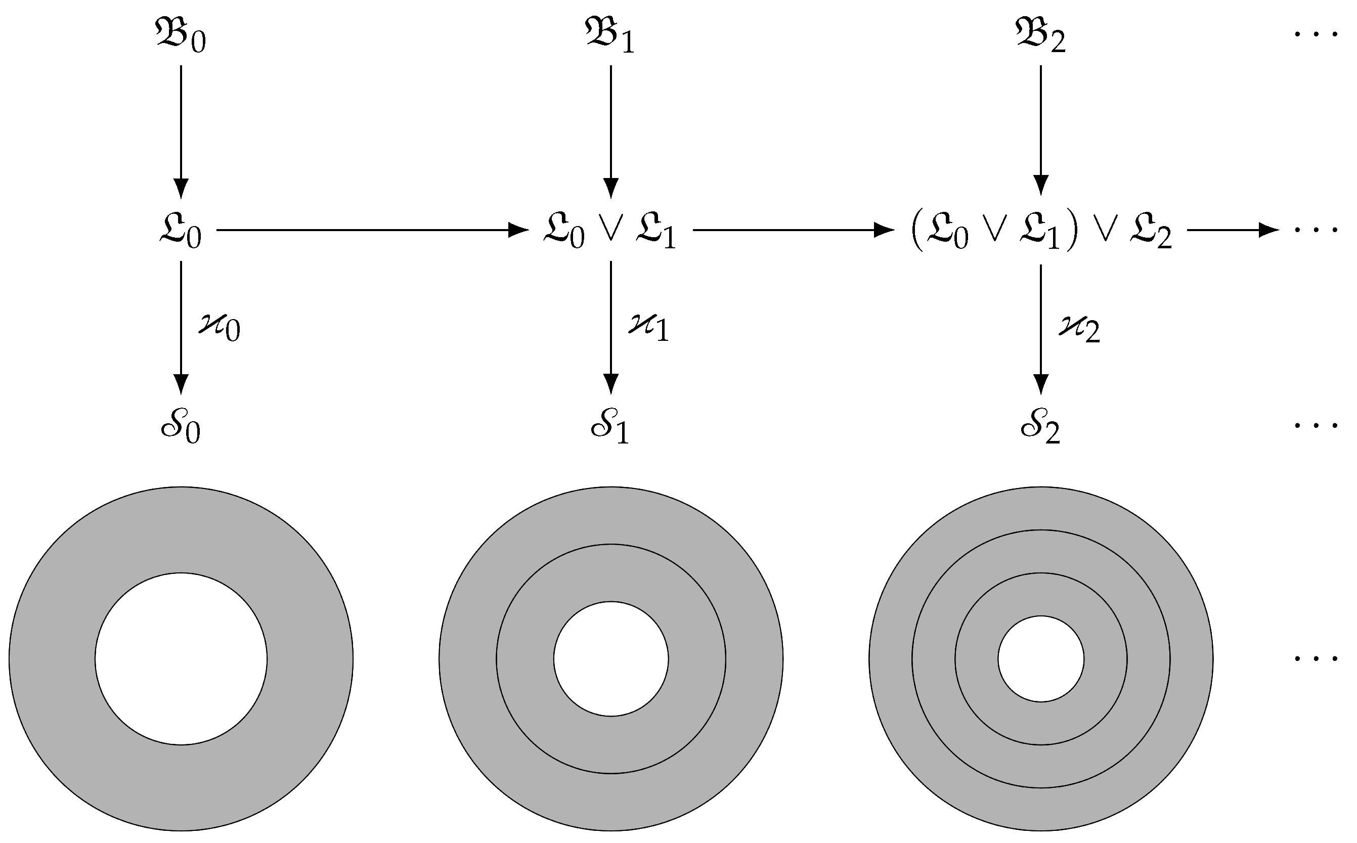
Hereafter the stand-alone index n refers to the assembly number, while the pair of indexes, $n,k$, points to the assembly number n and the number k of the layer within the assembly. The relations between layers and assemblies are illustrated on Figure 1 (equatorial sections are shown). The mapping ${\varkappa }_n:{\mathfrak{B}}_n\to \mathcal{E}$, $n\in \{0,\cdots ,N\}$, is the actual configuration.

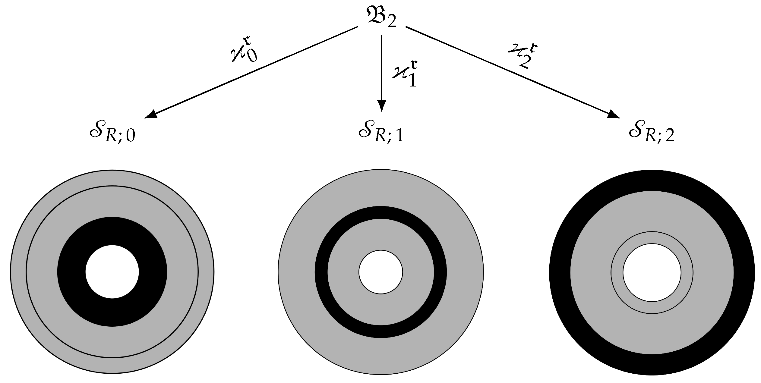
It is assumed that for every value $k\in \{0,\cdots ,N\}$ one can find configuration ${\varkappa }_k^{\mathfrak{r}}:{\mathfrak{B}}_N\to \mathcal{E}$ of the final body, that transforms the layer ${\mathfrak{L}}_k\subset {\mathfrak{B}}_N$ into stress-free shape ${\mathcal{L}}_k={\varkappa }_k^{\mathfrak{r}}\left({\mathfrak{L}}_k\right)$ which, as a region in $\mathcal{E}$, is a hollow ball:

$${\mathcal{L}}_k=\{x\in \mathcal{E}|{\mathfrak{r}}_k^i<\parallel x-\mathcal{O}\parallel <{\mathfrak{r}}_k^{\mathit{e}}\}.$$

For $N=2$ this assumption is illustrated on Figure 2. Symbols ${\mathcal{S}}_{R;k}$, $k=0,1,2$, denote shapes of the body ${\mathfrak{B}}_{\mathfrak{2}}$, that contain stress-free shapes ${\mathcal{L}}_k$ of layers. The layers, highlighted by black in corresponding shape of the assembly, are in stress-free state. Note, that the remaining parts of the whole shape, generally, are stressed.

Internal and external radii ${\mathfrak{r}}_0^i$, ${\mathfrak{r}}_0^{\mathit{e}}$, of the initial body are known, while internal, ${\mathfrak{r}}_{n+1}^i$, and external, ${\mathfrak{r}}_{n+1}^{\mathit{e}}$, radii of stress-free shape of ${\mathfrak{L}}_{n+1}$ are need to be determined. We suppose that the process is performed in two stages. Assume that we already have obtained internal, $r_{n,n}^i$, and external, $r_{n,n}^{\mathit{e}}$, actual radii of the layer ${\mathfrak{L}}_n$. At first stage, the layer ${\mathfrak{L}}_{n+1}$ is joined to the body ${\mathfrak{B}}_n$. The internal, ${\tilde{r}}_{n+1,n+1}^i$, and external, ${\tilde{r}}_{n+1,n+1}^{\mathit{e}}$, radii of the joined layer are set to be equal:

$${\tilde{r}}_{n+1,n+1}^i=r_{n,n}^{\mathit{e}},{\tilde{r}}_{n+1,n+1}^{\mathit{e}}={\tilde{r}}_{n+1,n+1}^i+{\mathrm{\Delta }}_{n+1},$$

where ${\mathrm{\Delta }}_{n+1}$ is the prescribed thickness. At the second stage, the layer ${\mathfrak{L}}_{n+1}$ is subjected to shrinkage with parameter ${\zeta }_{n+1}$:

$${\mathfrak{r}}_{n+1}^i={\zeta }_{n+1}{\tilde{r}}_{n+1,n+1}^i,{\mathfrak{r}}_{n+1}^{\mathit{e}}={\zeta }_{n+1}{\tilde{r}}_{n+1,n+1}^{\mathit{e}}.$$

These two stages are closely related with technological process, when thin polymeric film is joined to the substrate and is subjected to UV-radiation after joining [3]. As it would be shown in the paper, the knowledge of reference radii ${\mathfrak{r}}_0^i$, ${\mathfrak{r}}_0^{\mathit{e}}$ of the initial body, intermediate thicknesses ${\mathrm{\Delta }}_{n+1}$ and shrinkage parameters ${\zeta }_{n+1}$, as well as the central symmetry of deformations allow one to obtain all reference radii successively, during solution of evolutionary problem.

2.2. Coordinates and Deformation

Coordinates. Due to Euclidean structure of the physical space one can introduce Cartesian frame $(\mathcal{O};{\left(i_s\right)}_{s=1}^3)$ where $\mathcal{O}\in \mathcal{E}$ is the origin and ${\left(i_s\right)}_{s=1}^3$ is an orthonormal basis: $i_s\in \mathcal{V}$, $s\in \{1,2,3\}$ and $i_s·i_p={\delta }_{sp}$. The symbol ${\delta }_{sp}$ is the Kronecker delta. To benefit from central symmetry, proposed for all shapes, it would be worthwhile to adopt a spherical chart $(r,\theta ,\phi )$ that related with Cartesian one, $(x^1,x^2,x^3)$, as

$$x^1=rsin\theta cos\phi ,x^2=rsin\theta sin\phi ,x^3=rcos\theta ,$$

(3)

where $r>0$, $\theta \in ]0,\pi [$, $\phi \in [0,2\pi [$. The coordinates of the places, occupied by points within the shape ${\mathcal{L}}_k$, are denoted by $({\mathfrak{r}}_k,{\mathfrak{t}}_k,{\mathfrak{f}}_k)$, while the coordinates of places, occupied by the same points within the shape ${\mathcal{S}}_n$ are denoted by $(r_n,{\theta }_n,{\phi }_n)$. The field of local bases, related with spherical chart, will be denoted by $({\mathit{e}}_r,{\mathit{e}}_{\theta },{\mathit{e}}_{\phi })$. For the elements of the corresponding field of dual bases we use the following notation: $({\mathit{e}}^r,{\mathit{e}}^{\theta },{\mathit{e}}^{\phi })$ (Recall that ${\mathit{e}}_c={\displaystyle \frac{\partial x^k}{\partial c}}{i}_k$, ${\mathit{e}}^s·{\mathit{e}}_c={\delta }_c^s=\left\{\begin{array}{cc}1,\hfill & s=c\hfill \\ 0,\hfill & s\ne c.\hfill \end{array}\right.$; $s,c\in \{r,\theta ,\phi \}$.).

Representation of deformation. In view of central symmetry of deformations ${\gamma }_{n,k}:{\mathcal{L}}_k\to {\mathcal{S}}_n$, one can obtain the coordinate representation for them in the following form:

$${\tilde{\gamma }}_{n,k}=\psi \circ {\gamma }_{n,k}\circ {\psi }^{-1}:({\mathfrak{r}}_k,{\mathfrak{t}}_k,{\mathfrak{f}}_k)\mapsto (r_n,{\theta }_n,{\phi }_n),$$

where $\psi :x\mapsto (r,\theta ,\phi )$ is spherical coordinate map,

$$r_n=u_{n,k}\left({\mathfrak{r}}_k\right),{\theta }_n={\mathfrak{t}}_k,{\phi }_n={\mathfrak{f}}_k.$$

(4)

It is supposed that functions $u_{n,k}:[{\mathfrak{r}}_k^i,{\mathfrak{r}}_k^{\mathit{e}}]\to [r_{n,k}^i,r_{n,k}^{\mathit{e}}]$, which return the distance from the frame origin $\mathcal{O}$ to actual positions of material particles within the shape ${\mathcal{L}}_{n,k}$, are diffeomorphisms.

2.3. Strain Measures

Deformation gradient and left Cauchy–Green strain. Under the assumptions stated above one can define the deformation gradient ${\mathit{F}}_{n,k}=D{\gamma }_{n,k}:{\mathcal{L}}_k\to \mathrm{Lin}(\mathcal{V};\mathcal{V})$ as diagonal dyadic decomposition at a point $\mathcal{X}\in {\mathcal{L}}_k$:

$${\mathit{F}}_{n,k}{|}_{\mathcal{X}}=u_{n,k}^{\prime }\left({\mathfrak{r}}_k\right){\mathit{e}}_r{|}_{{\gamma }_{n,k}\left(\mathcal{X}\right)}\otimes {\mathit{e}}^r{|}_{\mathcal{X}}+{\mathit{e}}_{\theta }{|}_{{\gamma }_{n,k}\left(\mathcal{X}\right)}\otimes {\mathit{e}}^{\theta }{|}_{\mathcal{X}}+{\mathit{e}}_{\phi }{{|}_{{\gamma }_{n,k}\left(\mathcal{X}\right)}\otimes {\mathit{e}}^{\phi }|}_{\mathcal{X}}.$$

(5)

We use here vertical bars after base elements to clarify that they are defined with respect to spatial positions $\mathcal{X}$ or ${\gamma }_{n,k}\left(\mathcal{X}\right)$. Here and in what follows the symbol $\mathrm{Lin}(U;V)$ denotes the vector space of linear mappings from U to V. The symbol D in $D{\gamma }_{n,k}$ means operation of derivative applied to point-to-point mapping ${\gamma }_{n,k}$. That is, for any point $\mathcal{X}\in {\mathcal{L}}_k$ and for every translation vector $\mathit{h}\in \mathcal{V}$, sufficiently small, one has ${\gamma }_{n,k}(\mathcal{X}+\mathit{h})={\gamma }_{n,k}\left(\mathcal{X}\right)+D{\gamma }_{n,k}{|}_{\mathcal{X}}\left[\mathit{h}\right]+\mathit{o}(\parallel \mathit{h}\parallel )$. The discussion on various dyadic representations of deformation gradient ${\mathit{F}}_{n,k}=D{\gamma }_{n,k}$ can be found in [24].

Remaining within the classical provisions of continuum mechanics and taking into account the principle of material frame indifference [52], in what follows, instead of deformation gradient ${\mathit{F}}_{n,k}$, we use left Cauchy–Green strain tensor ${\mathit{B}}_{n,k}$ defined as ${\mathit{B}}_{n,k}={\mathit{F}}_{n,k}{\mathit{F}}_{n,k}^{\mathrm{T}}$, where ${\mathit{F}}_{n,k}^{\mathrm{T}}$ is the transpose for ${\mathit{F}}_{n,k}$ (That is, $\mathit{v}·{\mathit{F}}_{n,k}\left[u\right]=u·{\mathit{F}}_{n,k}^{\mathrm{T}}\left[\mathit{v}\right]$, for all vectors $u,\mathit{v}\in \mathcal{V}$.), which dyadic representation is (This representation is based on the following: (1) the dyads ${\mathit{e}}_i{{|}_{\mathcal{X}}\otimes {\mathit{e}}^j|}_{{\gamma }_{n,k}\left(\mathcal{X}\right)}$ were chosen (note, that they differ from dyads ${\mathit{e}}_i{{|}_{{\gamma }_{n,k}\left(\mathcal{X}\right)}\otimes {\mathit{e}}^j|}_{\mathcal{X}}$ used for deformation gradient), (2) the matrix of metric tensor $g$ in spherical coordinates is diagonal, (3) the matrix of ${\mathit{F}}_{n,k}$, as it can be seen from (5), is diagonal, (4) the coordinate representation (4) of ${\gamma }_{n,k}$ is used.)

$$\begin{array}{cc}{\mathit{F}}_{n,k}^{\mathrm{T}}{|}_{\mathcal{X}}=u_{n,k}^{\prime }\left({\mathfrak{r}}_k\right){\mathit{e}}_r{{|}_{\mathcal{X}}\otimes {\mathit{e}}^r|}_{{\gamma }_{n,k}\left(\mathcal{X}\right)}+\hfill & \\ & \hfill +{\left({\displaystyle \frac{u_{n,k}\left({\mathfrak{r}}_k\right)}{{\mathfrak{r}}_k}}\right)}^2\left({\mathit{e}}_{\theta }{|}_{\mathcal{X}}\otimes {\mathit{e}}^{\theta }{|}_{{\gamma }_{n,k}\left(\mathcal{X}\right)}+{\mathit{e}}_{\phi }{{|}_{\mathcal{X}}\otimes {\mathit{e}}^{\phi }|}_{{\gamma }_{n,k}\left(\mathcal{X}\right)}\right),\end{array}$$

for $\mathcal{X}\in {\mathcal{L}}_k$. Thus, we obtain the following decompositions for left Cauchy–Green strain tensor ${\mathit{B}}_{n,k}$ and its inverse, ${\mathit{B}}_{n,k}^{-1}$ (Note, that both decompositions are expressed in terms of dyads ${\mathit{e}}_i\otimes {\mathit{e}}^j$. The reason is the choice for the dyadic representation for the transpose ${\mathit{F}}_{n,k}^{\mathrm{T}}$. Another choice of the dyads (which can be performed by virtue of Euclidean structure of translation space $\mathcal{V}$), e.g., ${\mathit{e}}_i\otimes {\mathit{e}}_j$, would result in different representation for ${\mathit{B}}_{n,k}$.):

$$\begin{array}{cc}\hfill {\mathit{B}}_{n,k}& ={\left(u_{n,k}^{\prime }\right)}^2{\mathit{e}}_r\otimes {\mathit{e}}^r+{\left({\displaystyle \frac{u_{n,k}}{{\mathfrak{r}}_k}}\right)}^2{\mathit{e}}_{\theta }\otimes {\mathit{e}}^{\theta }+{\left({\displaystyle \frac{u_{n,k}}{{\mathfrak{r}}_k}}\right)}^2{\mathit{e}}_{\phi }\otimes {\mathit{e}}^{\phi },\hfill \end{array}$$

(6)

$$\begin{array}{cc}\hfill {\mathit{B}}_{n,k}^{-1}& ={\left({\displaystyle \frac{1}{u_{n,k}^{\prime }}}\right)}^2{\mathit{e}}_r\otimes {\mathit{e}}^r+{\left({\displaystyle \frac{{\mathfrak{r}}_k}{u_{n,k}}}\right)}^2{\mathit{e}}_{\theta }\otimes {\mathit{e}}^{\theta }+{\left({\displaystyle \frac{{\mathfrak{r}}_k}{u_{n,k}}}\right)}^2{\mathit{e}}_{\phi }\otimes {\mathit{e}}^{\phi }.\hfill \end{array}$$

(7)

Note that the components of decompositions above depend on the values of functions $u_{n,k}$ and their derivatives, calculated at point $\mathcal{X}\in {\mathcal{L}}_k$, while the dyads ${\mathit{e}}_i\otimes {\mathit{e}}^j$ are composed by the elements of local bases, corresponded to spherical chart at point ${\gamma }_{n,k}\left(\mathcal{X}\right)$ of the shape ${\mathcal{L}}_{n,k}$.

Within the paper only isotropic materials are considered. In this regard the response can be formalized as the function of principal invariants of ${\mathit{B}}_{n,k}$. Taking (6) into account, it is easy to represent them in terms of functions $u_{n,k}$ and their derivatives as:

$$\begin{array}{cc}\hfill {\mathit{I}}_{n,k}^{\left(1\right)}& =\mathrm{tr}{\mathit{B}}_{n,k}={\left(u_{n,k}^{\prime }\right)}^2+2{\left({\displaystyle \frac{u_{n,k}}{{\mathfrak{r}}_k}}\right)}^2,\hfill \\ \hfill {\mathit{I}}_{n,k}^{\left(2\right)}& ={\displaystyle \frac{1}{2}}\left(\mathrm{tr}{}^2{\mathit{B}}_{n,k}-\mathrm{tr}{\mathit{B}}_{n,k}^2\right)=2{\left(u_{n,k}^{\prime }\right)}^2{\left({\displaystyle \frac{u_{n,k}}{{\mathfrak{r}}_k}}\right)}^2+{\left({\displaystyle \frac{u_{n,k}}{{\mathfrak{r}}_k}}\right)}^4,\hfill \\ \hfill {\mathit{I}}_{n,k}^{\left(3\right)}& =det{\mathit{B}}_{n,k}={\left(u_{n,k}^{\prime }\right)}^2{\left({\displaystyle \frac{u_{n,k}}{{\mathfrak{r}}_k}}\right)}^4.\hfill \end{array}$$

(8)

2.4. Compressible Material

Compressible Mooney–Rivlin solid. To obtain results which can be applicable for numerical analysis, specify the general representation for elastic potential $W_{n,k}({\mathit{I}}_{n,k}^{\left(1\right)},{\mathit{I}}_{n,k}^{\left(2\right)},$${\mathit{I}}_{n,k}^{\left(3\right)})$ in three-parametric Mooney–Rivlin form (Note that hyperelastic models of compressible and incompressible materials allow one to describe deformation of real solids, in particular, of rubber, with high accuracy [53]. Rubber-like polymeric materials, that are frequently used in stereolithography, also belong to such class of media.)

$$W_{n,k}=C_1\left(J_{n,k}^{-2/3}{\mathit{I}}_{n,k}^{\left(1\right)}-3\right)+C_2\left(J_{n,k}^{-4/3}{\mathit{I}}_{n,k}^{\left(2\right)}-3\right)+{\displaystyle \frac{d}{2}}{(J_{n,k}-1)}^2,$$

(9)

$$J_{n,k}=det{\mathit{F}}_{n,k}=u_{n,k}^{\prime }{\left(u_{n,k}/{\mathfrak{r}}_k\right)}^2.$$

where $C_1$, $C_2$ and d are parameters that define the elastic properties of the material. Note that the parameters $C_1$, $C_2$ and d can be expressed in terms of “engineering” elastic moduli: $C_1=(1+b)\mu /4$, $C_2=(1-b)\mu /4$, where $\mu$ is a shear modulus, b is specific coefficient related with nonlinear behavior of the material, while d is a bulk modulus in the limit of small strains.

One can calculate Cauchy stress tensor ${\mathit{T}}_{n,k}$ with Doyle–Ericksen relation [52]

$${\mathit{T}}_{n,k}={\displaystyle \frac{2}{J_{n,k}}}{\mathit{B}}_{n,k}{\displaystyle \frac{\partial W_{n,k}}{\partial {\mathit{B}}_{n,k}}}={\beth }_0\mathit{I}+{\beth }_1{\mathit{B}}_{n,k}+{\beth }_{-1}{\mathit{B}}_{n,k}^{-1},$$

(10)

where ${\beth }_0$, ${\beth }_1$, ${\beth }_{-1}$ are scalar response functions,

$$\begin{array}{cc}{\beth }_0=2{\displaystyle \frac{\partial W_{n,k}}{\partial i_2}}{\mathit{I}}_{n,k}^{\left(2\right)}{\left({\mathit{I}}_{n,k}^{\left(3\right)}\right)}^{-1/2}\hfill & +2{\displaystyle \frac{\partial W_{n,k}}{\partial i_3}}{\left({\mathit{I}}_{n,k}^{\left(3\right)}\right)}^{1/2}=\hfill \\ & ={\displaystyle \frac{3d\left({\left({\mathit{I}}_{n,k}^{\left(3\right)}\right)}^{1/2}-1\right){\left({\mathit{I}}_{n,k}^{\left(3\right)}\right)}^{7/6}-2C_1{\mathit{I}}_{n,k}^{\left(1\right)}{\left({\mathit{I}}_{n,k}^{\left(3\right)}\right)}^{1/3}+2C_2{\mathit{I}}_{n,k}^{\left(2\right)}}{3{\left({\mathit{I}}_{n,k}^{\left(3\right)}\right)}^{7/6}}},\hfill \end{array}$$

$${\beth }_1=2{\displaystyle \frac{\partial W_{n,k}}{\partial i_1}}{\left({\mathit{I}}_{n,k}^{\left(3\right)}\right)}^{-1/2}={\displaystyle \frac{2C_1}{{\left({\mathit{I}}_{n,k}^{\left(3\right)}\right)}^{5/6}}},$$

(11)

$${\beth }_{-1}=-2{\displaystyle \frac{\partial W_{n,k}}{\partial i_2}}{\left({\mathit{I}}_{n,k}^{\left(3\right)}\right)}^{1/2}=-{\displaystyle \frac{2C_2}{{\left({\mathit{I}}_{n,k}^{\left(3\right)}\right)}^{1/6}}}.$$

After substitution of expressions (6), (7), (8) and (11) into (10) one can obtain the following formulas for Cauchy stresses in k-th layer within n-th assembly:

$${\mathit{T}}_{n,k}=\left({\mathit{T}}_{n,k}\right){}_r^r{\mathit{e}}_r\otimes {\mathit{e}}^r+\left({\mathit{T}}_{n,k}\right){}_{\theta }^{\theta }{\mathit{e}}_{\theta }\otimes {\mathit{e}}^{\theta }+\left({\mathit{T}}_{n,k}\right){}_{\phi }^{\phi }{\mathit{e}}_{\phi }\otimes {\mathit{e}}^{\phi },$$

(12)

where

$$\begin{array}{c}\left({\mathit{T}}_{n,k}\right){}_r^r={\displaystyle \frac{4}{3}}{\mathfrak{r}}_k^{-4}{J}_{n,k}^{-7/3}\{u_{n,k}^4\left({\displaystyle \frac{3}{4}}d{J}_{n,k}^{1/3}\left(J_{n,k}-1\right){\left(u_{n,k}^{\prime }\right)}^2-C_2\right)+\hfill \\ \hfill +C_1{\mathfrak{r}}_k^8{J}_{n,k}^{8/3}{u}_{n,k}^{-4}-{\mathfrak{r}}_k^2{u}_{n,k}^2\left(C_1{J}_{n,k}^{2/3}-C_2{\left(u_{n,k}^{\prime }\right)}^2\right)\},\end{array}$$

$$\begin{array}{c}\left({\mathit{T}}_{n,k}\right){}_{\phi }^{\phi }=\left({\mathit{T}}_{n,k}\right){}_{\theta }^{\theta }={\displaystyle \frac{2}{3}}{\mathfrak{r}}_k^{-4}{J}_{n,k}^{-7/3}\{u_{n,k}^4\left({\displaystyle \frac{3}{2}}d{J}_{n,k}^{1/3}\left(J_{n,k}-1\right){\left(u_{n,k}^{\prime }\right)}^2+C_2\right)-\hfill \\ \hfill -C_1{\mathfrak{r}}_k^8{J}_{n,k}^{8/3}{u}_{n,k}^{-4}+{\mathfrak{r}}_k^2{u}_{n,k}^2\left(C_1{J}_{n,k}^{2/3}-C_2{\left(u_{n,k}^{\prime }\right)}^2\right)\}.\end{array}$$

Boundary value problem. The Cauchy stress field (12) should meet the equilibrium condition $\mathrm{div}{\mathit{T}}_{n,k}=\mathbf{0}$ (here, $\mathrm{div}$ denotes divergence operation defined on actual shape ${\mathcal{S}}_n$), which, in a view of central symmetry, results in only one non-trivial scalar equation that can be written in actual coordinates as:

$${\displaystyle \frac{\partial \left({\mathit{T}}_{n,k}\right){}_r^r}{\partial r}}+{\displaystyle \frac{2}{r}}\left(\left({\mathit{T}}_{n,k}\right){}_r^r-\left({\mathit{T}}_{n,k}\right){}_{\theta }^{\theta }\right)=0,$$

(13)

where $\left({\mathit{T}}_{n,k}\right){}_r^r$ and $\left({\mathit{T}}_{n,k}\right){}_{\theta }^{\theta }$ can be regarded as shorthand for expressions (12). After the change of variables $r\mapsto {\mathfrak{r}}_k$ Equation (13) takes the form:

$${\displaystyle \frac{\partial \left({\mathit{T}}_{n,k}\right){}_r^r}{\partial {\mathfrak{r}}_k}}+2{\displaystyle \frac{u_{n,k}^{\prime }}{u_{n,k}}}\left(\left({\mathit{T}}_{n,k}\right){}_r^r-\left({\mathit{T}}_{n,k}\right){}_{\theta }^{\theta }\right)=0.$$

(14)

To complete the statement of the boundary-value problem (BVP) one has to specify boundary conditions on the interior and exterior boundaries of multilayered structure as well as on the interfaces between them. Again keeping in mind the central symmetry of discussed problem we assume that the outer boundaries of multilayered structure are homogeneously loaded with normal traction, i.e.,

$${\left.\left({\mathit{T}}_{n,0}\right){}_r^r\right|}_{r=r_{n,0}^i}=q_n^i,{\left.\left({\mathit{T}}_{n,n}\right){}_r^r\right|}_{r=r_{n,n}^{\mathit{e}}}=q_n^{\mathit{e}},$$

(15)

and on the interface surfaces between layers the ideal contact conditions hold:

$${\left.{\mathit{T}}_{n,k}·{\mathit{e}}^r\right|}_{r=r_{n,k}^{\mathit{e}}}={\left.{\mathit{T}}_{n,k+1}·{\mathit{e}}^r\right|}_{r=r_{n,k+1}^i},r_{n,k}^{\mathit{e}}=r_{n,k+1}^i.$$

(16)

The substitution of the relations (12) into Equation (14) and boundary conditions (15) and (16) after straightforward calculations results in the following quasilinear system of equations:

$$\begin{array}{c}\forall \mathfrak{r}\in ]{\mathfrak{r}}_k^i,{\mathfrak{r}}_k^{\mathit{e}}[:u_{n,k}^{″}+\mathrm{Y}(u_{n,k},u_{n,k}^{\prime })=0,\\ \mathrm{\Psi }(u_{n,0},u_{n,0}^{\prime }){|}_{\mathfrak{r}={\mathfrak{r}}_0^i}=q_n^i,\mathrm{\Psi }(u_{n,n},u_{n,n}^{\prime }){|}_{\mathfrak{r}={\mathfrak{r}}_n^{\mathit{e}}}=q_n^{\mathit{e}},\\ \forall k\in \{0,1,\cdots ,n-1\}:u_{n,k}{|}_{\mathfrak{r}={\mathfrak{r}}_k^{\mathit{e}}}=u_{n,k+1}{|}_{\mathfrak{r}={\mathfrak{r}}_{k+1}^i},\\ \mathrm{\Psi }(u_{n,k},u_{n,k}^{\prime }){|}_{\mathfrak{r}={\mathfrak{r}}_k^{\mathit{e}}}=\mathrm{\Psi }(u_{n,k+1},u_{n,k+1}^{\prime }){|}_{\mathfrak{r}={\mathfrak{r}}_{k+1}^i},\end{array}$$

(17)

where

$$\begin{array}{c}{\rm Y}(u,u^{\prime })=\hfill \\ {\left(\mathfrak{r}u\{u^8\left(9/4d{u}^{\prime 2}{J}^{4/3}-7C_2\right)+C_1{\mathfrak{r}}^8{J}^{8/3}+{\mathfrak{r}}^2{u}^6\left(5C_1{J}^{2/3}+C_2{u}^{\prime 2}\right)\}\right)}^{-1}\times \\ \times \left\{u^{\prime }\left(u-\mathfrak{r}{u}^{\prime }\right)(2u^8\left(C_2-9/4d{u}^{\prime 2}{J}^{4/3}\right)+C_1{\mathfrak{r}}^8{J}^{8/3}-9C_1{\mathfrak{r}}^3{u}^5{u}^{\prime }{J}^{2/3}-\right.\\ \hfill \left.-\{{\mathfrak{r}}^2{u}^6\left(4C_1{J}^{2/3}-C_2{u}^{\prime 2}\right)+9C_2\mathfrak{r}{u}^7{u}^{\prime }\})\right\},\end{array}$$

$$\begin{array}{c}\mathrm{\Psi }(u,u^{\prime })=2{\left(3u^8{u^{\prime }}^4\right)}^{-1}{J}^{5/3}\left({\mathfrak{r}}^4{u}^4\left(-3C_2{u^{\prime }}^6-C_2+3/2d{J}^{1/3}\left(J-1\right){u^{\prime }}^2\right)+\right.\hfill \\ \hfill \left.+{\mathfrak{r}}^8{u^{\prime }}^2\left(2C_1{J}^{2/3}+3C_2{u^{\prime }}^2\right)-2{\mathfrak{r}}^6{u}^2\left(C_1{J}^{2/3}+C_2{u^{\prime }}^2\right)+3C_2{u}^8{u^{\prime }}^2\right).\end{array}$$

Note that the reference radii ${\mathfrak{r}}_k^i$, ${\mathfrak{r}}_k^{\mathit{e}}$, $k=1,\cdots ,N$, of the layers, as well as their actual radii $r_{n,k}^i$, $r_{n,k}^{\mathit{e}}$ are initially unknown. All what we know are reference radii ${\mathfrak{r}}_0^i$, ${\mathfrak{r}}_0^{\mathit{e}}$ of the first layer, actual thicknesses ${\mathrm{\Delta }}_k$, $k=1,\cdots ,N$, of layers and the sine qua non for sequential joining: a new layer is always created upon the last one in already constituted assembly and just after creation it undergoes shrinkage with given ratio $\zeta$. In order to take the sequentiality into account one can consider the sequence of BVP that begins from the first one:

$$\begin{array}{c}\forall \mathfrak{r}\in ]{\mathfrak{r}}_0^i,{\mathfrak{r}}_0^{\mathit{e}}[:u_{0,0}^{″}+{\rm Y}(u_{0,0},u_{0,0}^{\prime })=0,\\ \mathrm{\Psi }(u_{0,0},u_{0,0}^{\prime }){|}_{\mathfrak{r}={\mathfrak{r}}_0^i}=q_0^i,\mathrm{\Psi }(u_{0,0},u_{0,0}^{\prime }){|}_{\mathfrak{r}={\mathfrak{r}}_0^{\mathit{e}}}=q_0^{\mathit{e}},\end{array}$$

(18)

Since the initial radii ${\mathfrak{r}}_0^i$, ${\mathfrak{r}}_0^{\mathit{e}}$ of the first layer as well as the densities $q_0^i$, $q_0^{\mathit{e}}$ of normal loadings are given, this problem is correctly stated with respect to unknown function $u_{0,0}$. The solution of the problem (18) defines the actual outer radius of the first layer, $r_{0,0}^{\mathit{e}}=u_{0,0}\left({\mathfrak{r}}_0^{\mathit{e}}\right)$. Thus, after deposition to the first assembly, the actual inner and outer radii ${\tilde{r}}_{1,1}^i$ and ${\tilde{r}}_{1,1}^{\mathit{e}}$ of the second layer with given actual thickness ${\mathrm{\Delta }}_1$ are equal to:

$${\tilde{r}}_{1,1}^i=r_{0,0}^{\mathit{e}},{\tilde{r}}_{1,1}^{\mathit{e}}={\tilde{r}}_{1,1}^i+{\mathrm{\Delta }}_1.$$

The second layer acquires the shrinkage ${\zeta }_1$; its reference radii are equal to:

$${\mathfrak{r}}_1^i={\zeta }_1{\tilde{r}}_{1,1}^i,{\mathfrak{r}}_1^{\mathit{e}}={\zeta }_1{\tilde{r}}_{1,1}^{\mathit{e}},$$

while its actual radii $r_{1,1}^i$ and $r_{1,1}^{\mathit{e}}$ in assembly after shrinkage are unknown. With obtained results the second problem in sequence can be stated as follows:

$$\begin{array}{c}\forall \mathfrak{r}\in ]{\mathfrak{r}}_0^i,{\mathfrak{r}}_0^{\mathit{e}}[:u_{1,0}^{″}+\mathrm{Y}(u_{1,0},u_{1,0}^{\prime })=0,\\ \forall \mathfrak{r}\in ]{\mathfrak{r}}_1^i,{\mathfrak{r}}_1^{\mathit{e}}[:u_{1,1}^{″}+\mathrm{Y}(u_{1,1},u_{1,1}^{\prime })=0,\\ \mathrm{\Psi }(u_{1,0},u_{1,0}^{\prime }){|}_{\mathfrak{r}={\mathfrak{r}}_0^i}=q_1^i,\mathrm{\Psi }(u_{1,1},u_{1,1}^{\prime }){|}_{\mathfrak{r}={\mathfrak{r}}_1^{\mathit{e}}}=q_1^{\mathit{e}},\\ u_{1,0}{|}_{\mathfrak{r}={\mathfrak{r}}_0^{\mathit{e}}}=u_{1,1}{|}_{\mathfrak{r}={\mathfrak{r}}_1^i},\\ \mathrm{\Psi }(u_{1,0},u_{1,0}^{\prime }){|}_{\mathfrak{r}={\mathfrak{r}}_0^{\mathit{e}}}=\mathrm{\Psi }(u_{1,1},u_{1,1}^{\prime }){|}_{\mathfrak{r}={\mathfrak{r}}_1^i}.\end{array}$$

The above equations and boundary conditions constitute together the correct statement for BVP with respect to two unknown functions $u_{1,0}$ and $u_{1,1}$. One can obtain the solution of this BVP numerically and calculate the value for actual outer radius $r_{1,1}^{\mathit{e}}$ of the second assembly as $r_{1,1}^{\mathit{e}}=u_{1,1}\left({\mathfrak{r}}_1^{\mathit{e}}\right)$. The actual inner and outer radii ${\tilde{r}}_{2,2}^i$ and ${\tilde{r}}_{2,2}^{\mathit{e}}$ of the third layer after deposition to the second assembly are equal to:

$${\tilde{r}}_{2,2}^i=r_{1,1}^{\mathit{e}},{\tilde{r}}_{2,2}^{\mathit{e}}={\tilde{r}}_{2,2}^i+{\mathrm{\Delta }}_2.$$

The third layer acquires the shrinkage ${\zeta }_2$; its reference radii are equal to:

$${\mathfrak{r}}_2^i={\zeta }_2{\tilde{r}}_{2,2}^i,{\mathfrak{r}}_2^{\mathit{e}}={\zeta }_2{\tilde{r}}_{2,2}^{\mathit{e}},$$

while its actual radii $r_{2,2}^i$ and $r_{2,2}^{\mathit{e}}$ in assembly after shrinkage are unknown. The repetition of such evaluations results in n-th step to the BVP:

$$\begin{array}{c}\forall \mathfrak{r}\in ]{\mathfrak{r}}_0^i,{\mathfrak{r}}_0^{\mathit{e}}[:u_{n,0}^{″}+{\rm Y}(u_{n,0},u_{n,0}^{\prime })=0,\\ \forall \mathfrak{r}\in ]{\mathfrak{r}}_1^i,{\mathfrak{r}}_1^{\mathit{e}}[:u_{n,1}^{″}+{\rm Y}(u_{n,1},u_{n,1}^{\prime })=0,\\ \cdots \\ \forall \mathfrak{r}\in ]{\mathfrak{r}}_n^i,{\mathfrak{r}}_n^{\mathit{e}}[:u_{n,n}^{″}+{\rm Y}(u_{n,n},u_{n,n}^{\prime })=0,\\ \mathrm{\Psi }(u_{n,0},u_{n,0}^{\prime }){|}_{\mathfrak{r}={\mathfrak{r}}_0^i}=q_n^i,\mathrm{\Psi }(u_{n,n},u_{n,n}^{\prime }){|}_{\mathfrak{r}={\mathfrak{r}}_n^{\mathit{e}}}=q_n^{\mathit{e}},\\ u_{n,0}{|}_{\mathfrak{r}={\mathfrak{r}}_0^{\mathit{e}}}=u_{n,1}{|}_{\mathfrak{r}={\mathfrak{r}}_1^i},\mathrm{\Psi }(u_{n,0},u_{n,0}^{\prime }){|}_{\mathfrak{r}={\mathfrak{r}}_0^{\mathit{e}}}=\mathrm{\Psi }(u_{n,1},u_{n,1}^{\prime }){|}_{\mathfrak{r}={\mathfrak{r}}_1^i},\\ u_{n,1}{|}_{\mathfrak{r}={\mathfrak{r}}_1^{\mathit{e}}}=u_{n,2}{|}_{\mathfrak{r}={\mathfrak{r}}_2^i},\mathrm{\Psi }(u_{n,1},u_{n,1}^{\prime }){|}_{\mathfrak{r}={\mathfrak{r}}_1^{\mathit{e}}}=\mathrm{\Psi }(u_{n,2},u_{n,2}^{\prime }){|}_{\mathfrak{r}={\mathfrak{r}}_2^i},\\ \cdots \\ u_{n,n-1}{|}_{\mathfrak{r}={\mathfrak{r}}_{n-1}^{\mathit{e}}}=u_{n,n}{|}_{\mathfrak{r}={\mathfrak{r}}_n^i},\mathrm{\Psi }(u_{n,n-1},u_{n,n-1}^{\prime }){|}_{\mathfrak{r}={\mathfrak{r}}_{n-1}^{\mathit{e}}}=\mathrm{\Psi }(u_{n,n},u_{n,n}^{\prime }){|}_{\mathfrak{r}={\mathfrak{r}}_n^i},\end{array}$$

that is correctly stated with respect to sought functions $u_{n,0},u_{n,1},\cdots ,u_{n,n}$. The iterative evaluation is completed when the number n reaches the value N. In result we get the following sequences of functions:

$$\begin{array}{cc}\hfill & u_{0,0};\hfill \\ \hfill & u_{1,0},u_{1,1};\hfill \\ \hfill & u_{2,0},u_{2,1},u_{2,2};\hfill \\ \hfill & \cdots \hfill \\ \hfill & u_{N,0},u_{N,1},\cdots ,u_{N,N}.\hfill \end{array}$$

(19)

Each of these sequences defines the distribution of deformation parameters in layers within assemblies corresponded to certain steps of additive process.

2.5. Incompressible Material

Incompressible Mooney–Rivlin solid. Described above algorithm requires the application of some numerical method for solution of quasilinear two-point BVP at each step. To that end we use the shooting method [54] that demonstrates good convergency subject to the availability of fine initial approach. For problems under consideration one can obtain such fine initial approach as the solution of related BVP for incompressible material which is substantially simpler and allows for an analytical solution. The case of layers of incompressible homogeneous isotropic material is considered in [23] in detail. Here we present only an outline of main formulas.

Since $J_{n,k}=det{\mathit{F}}_{n,k}=u_{n,k}^{\prime }{\left(u_{n,k}/{\mathfrak{r}}_k\right)}^2=1$, one has ordinary differential equation $u_{n,k}^{\prime }{\left(u_{n,k}/{\mathfrak{r}}_k\right)}^2=1$. Its solution has the form:

$$r={[{\left({\mathfrak{r}}_k\right)}^3+a_{n,k}]}^{1/3},\theta ={\mathfrak{t}}_k,\phi ={\mathfrak{f}}_k,$$

and represents the particular case of the deformation law (4). Here $a_{n,k}$ are parameters of deformation that are constants.

Taking into account the central symmetry $]0,\infty [\ni r\mapsto x:x=\mathcal{O}+r{\mathit{e}}_r$, one can construct the mapping $]0,\infty [\ni r\mapsto {\mathit{B}}_{n,k}\left(r\right)$, which is the tilt of the left Cauchy–Green tensor field:

$${\mathit{B}}_{n,k}:{\mathcal{L}}_{n,k}\to \mathrm{Lin}(\mathcal{V};\mathcal{V}),{\mathit{B}}_{n,k}:{\mathcal{L}}_{n,k}\ni x\mapsto {\mathit{B}}_{n,k}\left(x\right)\in \mathrm{Lin}(\mathcal{V};\mathcal{V}).$$

Beyond that it is convenient to decompose tensor ${\mathit{B}}_{n,k}\left(x\right)$ in dyadic basis ${\mathit{e}}_i\otimes {\mathit{e}}^j$, generated by spherical chart at point $x$. All this results in the following representations for left Cauchy–Green tensor field and its inverse:

$$\begin{array}{cc}\hfill {\mathit{B}}_{n,k}& ={\displaystyle \frac{{(r^3-a_{n,k})}^{4/3}}{r^4}}{\mathit{e}}_r\otimes {\mathit{e}}^r+{\displaystyle \frac{r^2}{{(r^3-a_{n,k})}^{2/3}}}\left({\mathit{e}}_{\theta }\otimes {\mathit{e}}^{\theta }+{\mathit{e}}_{\phi }\otimes {\mathit{e}}^{\phi }\right),\hfill \\ \hfill {\mathit{B}}_{n,k}^{-1}& ={\displaystyle \frac{r^4}{{(r^3-a_{n,k})}^{4/3}}}{\mathit{e}}_r\otimes {\mathit{e}}^r+{\displaystyle \frac{{(r^3-a_{n,k})}^{2/3}}{r^2}}\left({\mathit{e}}_{\theta }\otimes {\mathit{e}}^{\theta }+{\mathit{e}}_{\phi }\otimes {\mathit{e}}^{\phi }\right).\hfill \end{array}$$

Because of adopted incompressibility of the material, the functional (9) reduces to the expression:

$$W_{n,k}=C_1\left(I_{n,k}^{\left(1\right)}-3\right)+C_2\left(I_{n,k}^{\left(2\right)}-3\right),$$

where $C_1$ and $C_2$ are the same as in (9). Straightforward calculations, based on Doyle–Ericksen Formula (10), give the representation for Cauchy stress fields ${\mathit{T}}_{n,k}$ up to unknown scalar functions $p_{n,k}$ that define the hydrostatic (spherical) component of ${\mathit{T}}_{n,k}$:

$${\mathit{T}}_{n,k}=-p_{n,k}\mathit{I}+2C_1{\mathit{B}}_{n,k}-2C_2{\mathit{B}}_{n,k}^{-1}.$$

Boundary value problem. The functions $p_{n,k}$ can be found in closed form from the solution of two-point equilibrium BVP that consists of scalar Equation (13) and boundary conditions (15) and (16). This allows one to obtain the components of Cauchy stress tensor field ${\mathit{T}}_{n,k}$ [52]:

$$\begin{array}{cc}\hfill & \left({\mathit{T}}_{n,k}\right){}_r^r={\stackrel{0}{p}}_{n,k}+{\displaystyle \frac{C_1(5r^3-a_{n,k}){(r^3-a_{n,k})}^{2/3}-2C_2{r}^2(r^3+a_{n,k})}{r^4{(r^3-a_{n,k})}^{1/3}}},\hfill \\ \hfill & \left({\mathit{T}}_{n,k}\right){}_{\phi }^{\phi }=\left({\mathit{T}}_{n,k}\right){}_{\theta }^{\theta }=\left({\mathit{T}}_{n,k}\right){}_r^r+2{\displaystyle \frac{a_{n,k}(2r^3-a_{n,k})}{r^4{(r^3-a_{n,k})}^{4/3}}}\left(C_1{(r^3-a_{n,k})}^{2/3}+C_2{r}^2\right),\hfill \end{array}$$

(20)

where the constant ${\stackrel{0}{p}}_{n,k}$ plays role of hydrostatic component, while the constant $a_{n,k}$ plays role of deformation parameter.

The substitution of (20) into boundary conditions (15) and (16) results in system of nonlinear equations, which is algebraic counterpart for the system (17) of differential equations in compressible case. For initial body ($n=0$) the system contains two equations only:

$${\stackrel{0}{p}}_{0,0}+\mathcal{T}[{\mathfrak{r}}_0^i;a_{0,0}]=q_0^i,{\stackrel{0}{p}}_{0,0}+\mathcal{T}[{\mathfrak{r}}_0^{\mathit{e}};a_{0,0}]=q_0^{\mathit{e}}.$$

(21)

Hereinafter

$$\mathcal{T}[\mathfrak{r};a]={\displaystyle \frac{C_1(5{\mathfrak{r}}^3+4a){\mathfrak{r}}^2-2C_2{({\mathfrak{r}}^3+a)}^{2/3}({\mathfrak{r}}^3+2a)}{\mathfrak{r}{({\mathfrak{r}}^3+a)}^{4/3}}}.$$

In equations (21) radii ${\mathfrak{r}}_0^i$, ${\mathfrak{r}}_0^{\mathit{e}}$ are known as well as densities $q_0^i$, $q_0^{\mathit{e}}$ of normal loadings. Thus, the problem is correctly stated with respect to unknown parameters ${\stackrel{0}{p}}_{0,0}$ and $a_{0,0}$. The solution of the system (21) allows to obtain the actual outer radius of the first layer: $r_{0,0}^{\mathit{e}}={[{\left({\mathfrak{r}}_0^{\mathit{e}}\right)}^3+a_{0,0}]}^{1/3}$. In the next step, when the second layer is deposited to the first assembly, just before the solidification we have values:

$${\tilde{r}}_{1,1}^i=r_{0,0}^{\mathit{e}},{\tilde{r}}_{1,1}^{\mathit{e}}={\tilde{r}}_{1,1}^i+{\mathrm{\Delta }}_1,$$

for the actual inner and outer radii ${\tilde{r}}_{1,1}^i$ and ${\tilde{r}}_{1,1}^{\mathit{e}}$ of the second layer with known actual thickness ${\mathrm{\Delta }}_1$. Reference radii of the second layer are equal to:

$${\mathfrak{r}}_1^i={\zeta }_1{\tilde{r}}_{1,1}^i,{\mathfrak{r}}_1^{\mathit{e}}={\zeta }_1{\tilde{r}}_{1,1}^{\mathit{e}},$$

where ${\zeta }_1$ is the shrinkage which the layer undergoes after joining.

With known reference radii ${\mathfrak{r}}_1^i$ and ${\mathfrak{r}}_1^{\mathit{e}}$ the system of equations

$$\begin{array}{c}{\stackrel{0}{p}}_{1,0}+\mathcal{T}[{\mathfrak{r}}_0^i;a_{1,0}]=q_1^i,{\stackrel{0}{p}}_{1,1}+\mathcal{T}[{\mathfrak{r}}_1^{\mathit{e}};a_{1,1}]=q_1^{\mathit{e}},\\ {\stackrel{0}{p}}_{1,0}+\mathcal{T}[{\mathfrak{r}}_0^{\mathit{e}};a_{1,0}]={\stackrel{0}{p}}_{1,1}+\mathcal{T}[{\mathfrak{r}}_1^i;a_{1,1}],\\ {\left({\mathfrak{r}}_0^{\mathit{e}}\right)}^3+a_{1,0}={\left({\mathfrak{r}}_1^i\right)}^3+a_{1,1},\end{array}$$

for assembly with two layers is well-defined with respect to unknowns ${\stackrel{0}{p}}_{1,0}$, ${\stackrel{0}{p}}_{1,1}$, $a_{1,0}$ and $a_{1,1}$. Solving this system, we can calculate the actual outer radius of the second layer: $r_{1,1}^{\mathit{e}}={[{\left({\mathfrak{r}}_1^{\mathit{e}}\right)}^3+a_{1,1}]}^{1/3}$. After joining of the third layer, just before solidification, its instantaneous inner and outer radii are equal to:

$${\tilde{r}}_{2,2}^i=r_{1,1}^{\mathit{e}},{\tilde{r}}_{2,2}^{\mathit{e}}={\tilde{r}}_{2,2}^i+{\mathrm{\Delta }}_2,$$

respectively. Reference radii of the third layer can be calculated as follows:

$${\mathfrak{r}}_2^i={\zeta }_2{\tilde{r}}_{2,2}^i,{\mathfrak{r}}_2^{\mathit{e}}={\zeta }_2{\tilde{r}}_{2,2}^{\mathit{e}}.$$

In the n-th step we get the nonlinear algebraic system:

$$\begin{array}{c}{\stackrel{0}{p}}_{n,0}+\mathcal{T}[{\mathfrak{r}}_0^i;a_{n,0}]=q_n^i,{\stackrel{0}{p}}_{n,n}+\mathcal{T}[{\mathfrak{r}}_n^{\mathit{e}};a_{n,n}]=q_n^{\mathit{e}},\\ {\stackrel{0}{p}}_{n,0}+\mathcal{T}[{\mathfrak{r}}_0^{\mathit{e}};a_{n,0}]={\stackrel{0}{p}}_{n,1}+\mathcal{T}[{\mathfrak{r}}_1^i;a_{n,1}],\\ {\left({\mathfrak{r}}_0^{\mathit{e}}\right)}^3+a_{n,0}={\left({\mathfrak{r}}_1^i\right)}^3+a_{n,1},\\ \cdots \\ {\stackrel{0}{p}}_{n,n-1}+\mathcal{T}[{\mathfrak{r}}_{n-1}^{\mathit{e}};a_{n,n-1}]={\stackrel{0}{p}}_{n,n}+\mathcal{T}[{\mathfrak{r}}_n^i;a_{n,n}],\\ {\left({\mathfrak{r}}_{n-1}^{\mathit{e}}\right)}^3+a_{n,n-1}={\left({\mathfrak{r}}_n^i\right)}^3+a_{n,n},\end{array}$$

(22)

with unknowns ${\stackrel{0}{p}}_{n,0},{\stackrel{0}{p}}_{n,1},\cdots ,{\stackrel{0}{p}}_{n,n}$, $a_{n,0},a_{n,1},\cdots ,a_{n,n}$. The system (22) is well-defined since densities $q_n^i$, $q_n^{\mathit{e}}$ of normal loadings as well as reference radii ${\mathfrak{r}}_0^i,\cdots ,{\mathfrak{r}}_n^i$, ${\mathfrak{r}}_0^{\mathit{e}},\cdots ,{\mathfrak{r}}_n^{\mathit{e}}$, are known. The iterative process is completed when the step n reaches the value N. As a result, we arrive at the algebraic counterpart of (19):

$$\begin{array}{cc}\hfill & {\stackrel{0}{p}}_{0,0};a_{0,0};\hfill \\ \hfill & {\stackrel{0}{p}}_{1,0},{\stackrel{0}{p}}_{1,1};a_{1,0},a_{1,1};\hfill \\ \hfill & {\stackrel{0}{p}}_{2,0},{\stackrel{0}{p}}_{2,1},{\stackrel{0}{p}}_{2,2};a_{2,0},a_{2,1},a_{2,2};\hfill \\ \hfill & \cdots \hfill \\ \hfill & {\stackrel{0}{p}}_{N,0},{\stackrel{0}{p}}_{N,1},\cdots ,{\stackrel{0}{p}}_{N,N},a_{N,0},a_{N,1},\cdots ,a_{N,N}.\hfill \end{array}$$

Each of these rows completely determines the stress–strain state of the assembly in certain step of additive process.

The algebraic system (22) can be solved numerically. The solution of the related system for linear model may be chosen as the initial approach, i.e.,

$$\left({\mathit{T}}_{n,k}\right){}_r^r=q{\displaystyle \frac{{\mathfrak{r}}_2^3}{{\mathfrak{r}}_1^3-{\mathfrak{r}}_2^3}}\left({\displaystyle \frac{{\mathfrak{r}}_1^3}{{\mathfrak{r}}^3}}-1\right),\left({\mathit{T}}_{n,k}\right){}_{\theta }^{\theta }=-q{\displaystyle \frac{{\mathfrak{r}}_2^3}{{\mathfrak{r}}_1^3-{\mathfrak{r}}_2^3}}\left(1+{\displaystyle \frac{{\mathfrak{r}}_1^3}{2{\mathfrak{r}}^3}}\right).$$

Here q is hydrostatic loading, ${\mathfrak{r}}_1<{\mathfrak{r}}_2$ are reference radii of hollow ball.

3. Laminated Structure

Numerical simulation. Now we can use algorithms formulated above for numerical simulation of stress and strain distributions in additively produced bodies whose layers undergo shrinkage just after adhering. We will take this opportunity to clarify the question: can one approach discontinuous fields in multilayered structure by continuous distributions? Furthermore, if it is relevant, what inaccuracy should be expected? To answer these questions, a series of computations was fulfilled by following a strategy of decreasing thickness of a layer with fixed total thickness of the final assembly. To that end the stress–strain state of the assemblies with final number of layers equal to 5, 20, 50, 100 and 200 were numerically studied.

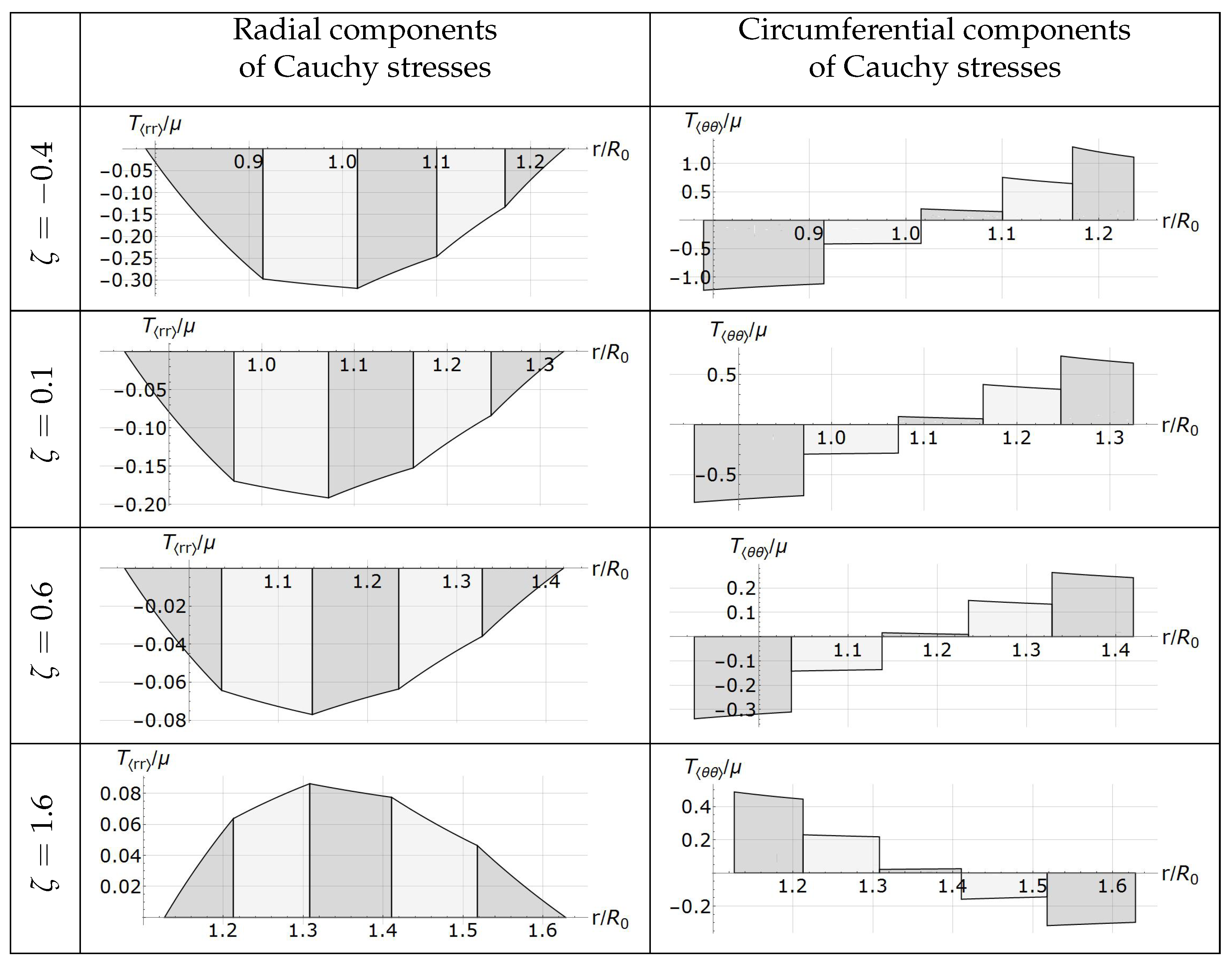
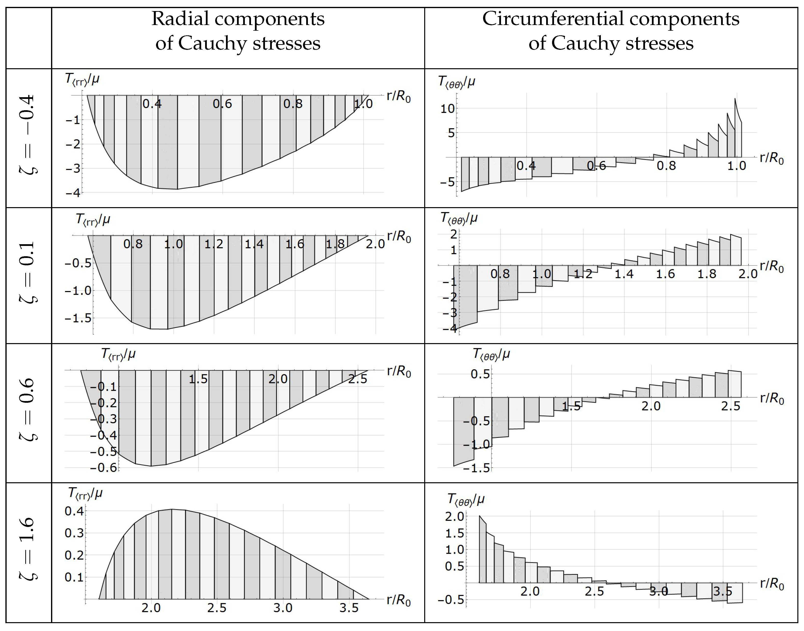
The distributions for the components of Cauchy stresses for the cases of 5 and 20 layers are shown on Figure 3 and Figure 4, respectively. Analysis of patterns of these distributions clearly demonstrates the possibility of continuous approach. Indeed, the most disturbing tendency to ebb and flow inherent in circumferential stresses, decreases with decreasing of a layer thickness. Actually, these distributions tend to functions that are not differentiable anywhere similar to well-known Weierstrass function [55] $w\left(x\right)={\sum }_{n=0}^{\infty }{a}^{n}cos\left(b^n\pi x\right)$, where $0<a<1$ and $b\ne 1$ is a positive odd number. However, the impact of such discontinuity decreases with increasing of total amount of layers.

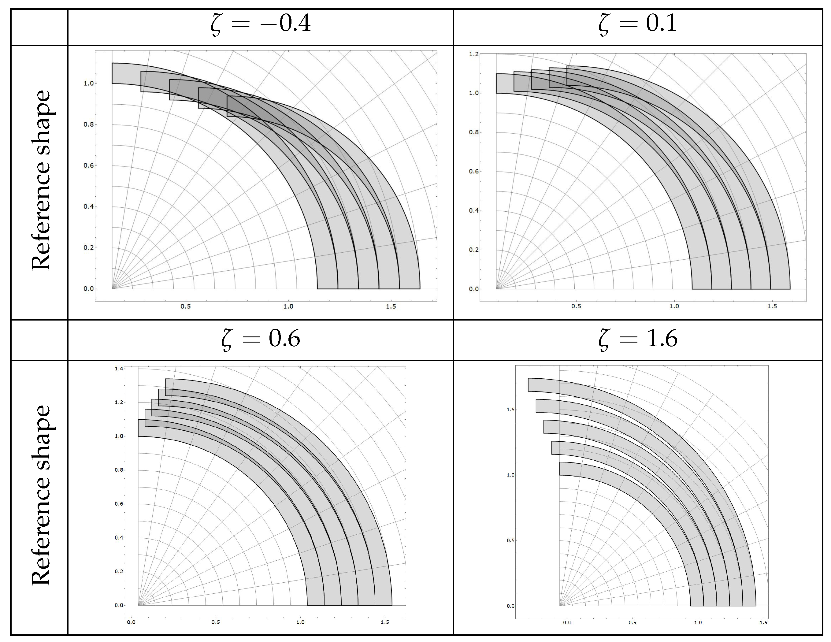
Considered examples of multilayered structures can be completely clarified within conventional non-linear elasticity. Meanwhile the reference shapes of final assemblies have some fairly unorthodox feature: they do not constitute a topologically connected sets. In this regard it is possible to image them as a number of regions that either overlap each other or can be situated with gaps. The pictorial representation of such alternatives is given in Figure 5. In this figure one can see quarters of equatorial section of spherical layers. They are placed in such a way that nearby layers touch each other in points on horizontal axis.

The provided analysis allows to draw the following conclusion: the continuous approach for multilayered structure with large number of thin layers is conceivable. All one has to do is to choose appropriate smoothing procedure. The simplest and natural way is the constructing of the approximation for deformation gradient ${\mathit{F}}_N$ with continuous functions, for instance, with polynomials.

Gluing. The representation of the totality of values ${\mathit{F}}_{N,k}$ (5) by a single field is rendered difficulty by a lack of connected domain, resulted in joining of individual domains for all ${\mathit{F}}_{N,k}$. Nevertheless, this difficulty can be overcome if such field will be defined piecewise from the “tilts” ${\mathit{F}}_{N,k}\circ g_{N,k}^{-1}$ of each individual field ${\mathit{F}}_{N,k}$ onto actual variables. Here $g_{N,k}:[r_{N,k}^i,r_{N,k}^{\mathit{e}}]\ni \mathfrak{r}\mapsto r\in [r_N^i,r_N^{\mathit{e}}]$ is the change of variables. Thus, we obtain the field ${\mathit{F}}_N:[r_N^i,r_N^{\mathit{e}}]\to \mathrm{Lin}(\mathcal{V};\mathcal{V})$,

$${\mathit{F}}_N=A_N{\mathit{e}}_r\otimes {\mathit{e}}^r+a_N{\mathit{e}}_{\theta }\otimes {\mathit{e}}^{\theta }+a_N{\mathit{e}}_{\phi }\otimes {\mathit{e}}^{\phi }.$$

(23)

where $A_N$ and $a_N$ are piecewise continuous distributions whose domains coincide with actual shape of final assembly (Coefficients of decomposition (5) are functions defined on the reference shape, while coefficients of decomposition (23) are defined on the actual shape. Both these decompositions represent one and the same deformation gradient in reference or actual variables, respectively):

$$A_N\left(r\right)=\left\{\begin{array}{cc}{\displaystyle \frac{1}{{\left\{u_{N,0}^{-1}\right\}}^{\prime }\left(r\right)}},\hfill & r\in {\mathit{I}}_{N,0},\hfill \\ \cdots \hfill & \cdots \hfill \\ {\displaystyle \frac{1}{{\left\{u_{N,N}^{-1}\right\}}^{\prime }\left(r\right)}},\hfill & r\in {\mathit{I}}_{N,N},\hfill \end{array}\right.a_N\left(r\right)=\left\{\begin{array}{cc}{\displaystyle \frac{r}{u_{N,0}^{-1}\left(r\right)}},\hfill & r\in {\mathit{I}}_{N,0},\hfill \\ \cdots \hfill & \cdots \hfill \\ {\displaystyle \frac{r}{u_{N,N}^{-1}\left(r\right)}},\hfill & r\in {\mathit{I}}_{N,N}.\hfill \end{array}\right.$$

Here we use designation ${\mathit{I}}_{N,k}=[r_{N,k}^i,r_{N,k}^{\mathit{e}}]$. So, in a manner of speaking, the field ${\mathit{F}}_N$ is obtained by “gluing” of individual deformation gradients ${\mathit{F}}_{N,k}\circ g_{N,k}^{-1}$, which had been made possible through the fact that the interiors of their domains do not intersect and in union results in an interval. Note, that except for a finite number of discontinuity points, the field ${\mathit{F}}_N$ represents compatible deformations from stress-free shapes of individual layers (which in combination do not constitute a joint set) into actual shape of final assembly.

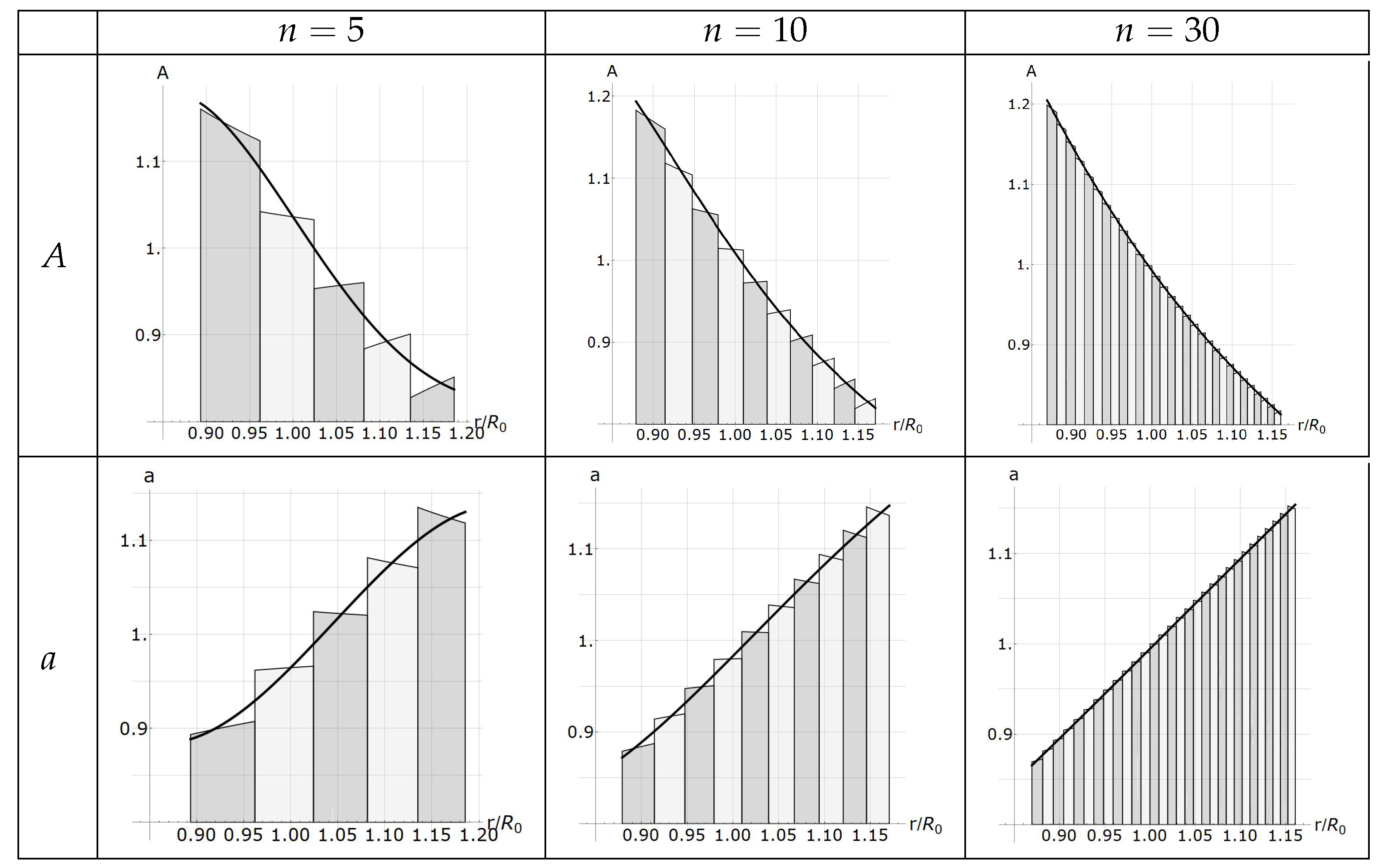
Smoothing. All is now ready to define the smooth counterpart to ${\mathit{F}}_N$ (23). This can be achieved with various averaging (smoothing) procedures. In present paper the polynomial averaging is used. It results in smooth tensorial field

$${\mathit{H}}^{-1}=A{\mathit{e}}_r\otimes {\mathit{e}}^r+a{\mathit{e}}_{\theta }\otimes {\mathit{e}}^{\theta }+a{\mathit{e}}_{\phi }\otimes {\mathit{e}}^{\phi }.$$

(24)

The field $\mathit{H}$ is referred to as distortion field. The components A and a of $\mathit{H}$ are smooth functions that are related with $A_N$ and $a_N$ by fourth-order spline interpolation. Note, that the field $\mathit{H}$, in general, represents incompatible local deformations, because functions A and a are no longer satisfy compatibility conditions. Consequently, there is no deformation that brings some stress-free shape onto actual one for final assembly, whose gradient would be equal to ${\mathit{H}}^{-1}$. It is easily shown that the result, i.e., the body ${\tilde{\mathfrak{B}}}_N$, whose actual shape coincides with ${\mathcal{S}}_N$ and local deformations, that bring the infinitesimal neighborhoods of its points into stress-free state, are defined by $\mathit{H}$, is nothing but a body with continuously distributed defects.

To compare stress–strain distributions the numerical analysis for assemblies with 5, 10, 30, 100 and 200 layers was provided. Total thicknesses of all layers within assemblies in stress-free state are equal to $0.3R_0$. For elastic moduli the following values were taken: $\lambda =2\mu$, $d=4\mu$, $b=\mu /2$, stress-free shapes of layers coincide with stress free shapes of the substrate (initial body), $q_n^i=q_n^{\mathit{e}}=0$.

The comparison of graphs of piecewise functions and approximations for 5, 10, 30 layers is shown on Figure 6. For more layers the graphs of these functions are typographically indistinguishable.

Laminated body. Due to the smoothing, the multilayered body ${\mathfrak{B}}_N$ is replaced by the laminated body ${\tilde{\mathfrak{B}}}_N$ with shape ${\mathcal{S}}_N$ and distortion tensor field $\mathit{H}$ defined on it. This field is inverse to (24) and provides the local relaxation of stressed state.

The formalization of the property that the body ${\tilde{\mathfrak{B}}}_N$ is laminated, i.e., it has foliated structure, may be performed in the framework of smooth bundles theory developed in differential geometry [56]. It is supposed that one can define a smooth trivial fiber bundle $({\tilde{\mathfrak{B}}}_N,\mathbb{I},\pi ,\mathfrak{F})$. Here $\mathbb{I}$ is a smooth one-dimensional base manifold, $\pi :{\tilde{\mathfrak{B}}}_N\to \mathbb{I}$ is a smooth surjective projection map and $\mathfrak{F}$ is a two-dimensional smooth fiber manifold.

It is assumed that the base $\mathbb{I}$ is a connected manifold, i.e., it cannot be disjoint union of two one-dimensional manifolds. Due to classification theorem for one-dimensional manifolds [57], $\mathbb{I}$ is either the unit circle ${\mathbb{S}}^1$ or the unit interval $]0,1[$. The first case corresponds to the cyclic process and then, in particular, the laminated body can be diffeomorphic to a solid torus. With certain loss of generality we restrict ourselves with the second case and put $\mathbb{I}=]0,1[$.

Each fiber ${\mathfrak{L}}_{\alpha }:={\pi }^{-1}\left(\left\{\alpha \right\}\right)$ is referred to as lamina [48]. The fact that $({\tilde{\mathfrak{B}}}_N,\mathbb{I},\pi ,\mathfrak{F})$ is fiber bundle implies that lamina ${\mathfrak{L}}_{\alpha }$ is two-dimensional submanifold of ${\tilde{\mathfrak{B}}}_N$, diffeomorphic to model fiber $\mathfrak{F}$. Moreover, the body ${\tilde{\mathfrak{B}}}_N$ is represented as the disjoint union

$${\tilde{\mathfrak{B}}}_N=\coprod _{\alpha \in ]0,1[}{\mathfrak{L}}_{\alpha },$$

of laminae ${\mathfrak{L}}_{\alpha }$, which completely reflects the property of being “laminated”. The spatial counterpart of such representation is that the actual shape ${\mathcal{S}}_N$ is a disjoint union of spheres.

According to the smoothing procedure, since the laminated body ${\tilde{\mathfrak{B}}}_N$ was obtained from the multilayered body ${\mathfrak{B}}_N$, which layers have stress-free shapes, then for each lamina ${\mathfrak{L}}_{\alpha }$ there exists configuration ${\varkappa }_{\alpha }^{\mathfrak{r}}:{\tilde{\mathfrak{B}}}_N\to \mathcal{E}$ such that Cauchy stress tensor $\mathit{T}$ vanishes at ${\varkappa }_{\alpha }^{\mathfrak{r}}\left({\mathfrak{L}}_{\alpha }\right)$. This allows one to synthesize the distortion tensor field, which coincides with field $\mathit{H}$ obtained from (24).

4. Non-Euclidean Stress-Free Shape

Euclidean reference and actual shapes. The shape of a body $\mathfrak{B}$ that can be observed in physical space $\mathcal{E}$, being three-dimensional submanifold of $\mathcal{E}$, inherits its geometrical properties such as metric, connection, surface and volume measures, as well as specific coordinate representations, related with particular charts that cover $\mathcal{E}$. This circumstance, that is perfect for conventional qualitative attributes of deformations that transform one region of ambient Euclidean space onto another, limits the potential to generalize the notion of deformations on non-Euclidean case. Meanwhile it would be unwise not to take advantage of Euclidean shapes, using their structure as “building blocks” for suitable definitions. To this end recall that smooth manifold, related with the body $\mathfrak{B}$ and physical space $\mathcal{E}$, can be regarded as following tuples [58,59]

$$\begin{array}{cc}\hfill \mathfrak{B}& =(\mathit{B},{\mathcal{T}}_{\mathit{B}},{\mathcal{D}}_{\mathit{B}}),\hfill \\ \hfill \mathcal{E}& =(E,{\mathcal{T}}_E,{\mathcal{D}}_E,g_E,{\nabla }_E).\hfill \end{array}$$

Here B and E are the basic elements of tuples, namely, underlying sets, which characterize the most fundamental properties of the structures. All that is required from them is to be of continuum cardinality. These sets are becoming topological spaces after introducing the corresponding collections ${\mathcal{T}}_{\mathit{B}}$, ${\mathcal{T}}_E$ of open subsets on them. The third elements of the tuples, ${\mathcal{D}}_{\mathit{B}}$, ${\mathcal{D}}_E$, endow B and E with smooth structures and turn them into smooth manifolds. At this stage no geometry is defined on B and E although the definition for the body manifold $\mathfrak{B}$ is being completed. Metric, that defines linear, surface and volume measures, and connection, related with parallel transport for vector fields and covariant differentiation, are specified on physical manifold $(E,{\mathcal{T}}_E,{\mathcal{D}}_E)$ with additional smooth fields $g_E$, and ${\nabla }_E$. Thereby, the body $\mathfrak{B}$, being no more than an abstract smooth manifold, is rather general, but, in the same time, poorer structure than the physical space $\mathcal{E}$.

The shapes of the body, being its images under smooth mappings (more precisely, embeddings [37]), which we refer to as configurations, are topologically indistinguishable from each other and from the body itself. If we treat them as an abstract smooth submanifolds of $\mathcal{E}$, all we got are some specific coordinate representation for them and, consequently, for the body itself, that we can glean from the spatial coordinates defined in some specific chart on physical space $\mathcal{E}$. However, we can give a more detailed description for the shapes, if we extend triples $(S,{\mathcal{T}}_S,{\mathcal{D}}_S)$, that define shapes, with specific metric and connection fields:

$$\mathtt{S}=(S,{\mathcal{T}}_S,{\mathcal{D}}_S,{\mathsf{g}}_S,{\nabla }_S),$$

where ${\mathcal{T}}_S$ and ${\mathcal{D}}_S$ are no more than restrictions of the formal objects defined on E to the region $S\subset E$ occupied by shape. In general, metric ${\mathsf{g}}_S$ and connection ${\nabla }_S$ are completely independent from the geometry, defined on $\mathcal{E}$. In this case we have non-Euclidean shape, that was already mentioned in Introduction. All what is in common among such shapes and physical space $\mathcal{E}$ are similarity of their topologies and possible sharing of coordinate charts, defined by spatial positions of points, that constitute particular shapes.

In specific case, related to conventional considerations in continuum mechanics, metric and connection on a shape are induced by geometry, defined in physical space $\mathcal{E}$, that can be done as follows:

$$\mathcal{S}=(S,{\mathcal{T}}_S,{\mathcal{D}}_S,{\iota }_S^{*}{g}_E,{\iota }_S^{*}{\nabla }_E).$$

Here ${\iota }_S:S\to E$ is the inclusion map and ${\iota }_S^{*}$ denotes pullback operation [36]. If we use the same coordinate representation on the shape $\mathcal{S}$ and physical space $\mathcal{E}$ then we obtain in coordinate form completely the same definitions of all geometric properties of $\mathcal{E}$, only narrowed on the region, occupied by S:

$$\mathcal{S}=(S,{\mathcal{T}}_S,{\mathcal{D}}_S,g_E{|}_S,{\nabla }_E{|}_S).$$

Here it is taken into account that the shape of the body, as well as physical space, have the same dimensions. One can do things slightly differently: he can share coordinate representation with one shape, say ${\mathcal{S}}_R$ (“reference shape”), and glean metric from another one, say ${\mathcal{S}}_t$ (“actual shape”), by pullback transformation:

$$g_{{\mathcal{S}}_R}={\gamma }^{*}{g}_{{\mathcal{S}}_t},g_{{\mathcal{S}}_R}(u,\mathit{v}):=g_{{\mathcal{S}}_t}\left(D\gamma \left[u\right],D\gamma \left[\mathit{v}\right]\right),$$

where $\gamma :{\mathcal{S}}_R\to {\mathcal{S}}_t$ is the deformation that brings ${\mathcal{S}}_R$ to ${\mathcal{S}}_t$. This results into two different tensor fields: the first one, ${\mathit{G}}_{{\mathcal{S}}_R}=g_E{|}_{S_R}$, corresponds to reference metric, while the second, $g_{{\mathcal{S}}_R}$, determines the metric of actual (deformed) shape. The difference $g_{{\mathcal{S}}_R}-{\mathit{G}}_{{\mathcal{S}}_R}$ between them represents conventional strain measure.

The connection also can be either duplicated or gleaned from another shape with pullback transformation [60]:

$${\nabla }_{{\mathcal{S}}_R}={\gamma }^{*}{\nabla }_{{\mathcal{S}}_t},{\left({\nabla }_{{\mathcal{S}}_R}\right)}_u\mathit{v}:={\gamma }^{*}\left\{{\left({\nabla }_{{\mathcal{S}}_t}\right)}_{{\gamma }_{*}u}\left({\gamma }_{*}\mathit{v}\right)\right\},$$

where $u$, $\mathit{v}$ are vector fields on ${\mathcal{S}}_R$, $\gamma :{\mathcal{S}}_R\to {\mathcal{S}}_t$ is the deformation and ${\gamma }^{*}$, ${\gamma }_{*}$ denote pullback and pushforward of vector fields [36] (Pullback and pushforward are operations defined for arbitrary smooth manifolds. Below we use the fact that the space is Euclidean and shapes are three-dimensional as well as the physical space. Meanwhile, in general, one needs to use tangent map operation T instead of total derivative D.):

$$\begin{array}{cc}\hfill {\gamma }^{*}u& =\left(D{\gamma }^{-1}\right)\circ u\circ \gamma ,\hfill \\ \hfill {\gamma }_{*}\mathit{v}& =\left(D\gamma \right)\circ \mathit{v}\circ {\gamma }^{-1},\hfill \end{array}$$

for vector field $u$ on ${\mathcal{S}}_t$ and vector field $\mathit{v}$ on ${\mathcal{S}}_R$. In standard textbooks covariant derivative, defined by connection ${\nabla }_E{|}_S$ is referred to as reference nabla operator, while its counterpart, defined by connection ${\gamma }^{*}{\nabla }_{{\mathcal{S}}_t}$, as spatial nabla operator [61]. Thus, we obtain at least two alternatives to introduce geometry on a shape in conventional way:

$$\begin{array}{cc}\hfill {\mathcal{S}}_R& =(S_R,{\mathcal{T}}_{S_R},{\mathcal{D}}_{S_R},g_E{|}_{S_R},{\nabla }_E{|}_{S_R}),\hfill \\ \hfill {\mathcal{S}}_R^{\prime }& =(S_R,{\mathcal{T}}_{S_R},{\mathcal{D}}_{S_R},{\gamma }^{*}{g}_{{\mathcal{S}}_t},{\gamma }^{*}{\nabla }_{{\mathcal{S}}_t}).\hfill \end{array}$$

All of them are used in conventional continuum mechanics. Obviously the manifold $(S_R,{\mathcal{T}}_{S_R},{\mathcal{D}}_{S_R})$, geometrized in such a manner, conserves the qualitative properties of ambient physical space $\mathcal{E}$. In particular, since $\mathcal{E}$ is Euclidean, then all two defined above ${\mathcal{S}}_R$’s are Euclidean spaces also.

Meanwhile one can use another way of thinking, regarding local deformation $\mathit{H}$ as linear transformation of vectorial triads ${\left({\mathit{e}}_i\right)}_{i=1}^3$, induced on reference shape ${\mathcal{S}}_R$ by local coordinate bases in physical space $\mathcal{E}$. Generally, new fields ${\left(z_i\right)}_{i=1}^3$ of vectorial triads determine some new connection, or, in other words, infinitesimal transport for vector fields, or, alternatively, covariant differentiation, that all relates to so called space with absolute parallelism [62]:

$${\nabla }_{z_i}{z}_j=\mathbf{0},i,j=1,2,3.$$

However, if such transformations are no more than total derivative $D\gamma$ of some smooth function $\gamma :{\mathcal{S}}_R\to \mathcal{E}$ that acts on coordinates shared by ${\mathcal{S}}_R$ and $\mathcal{E}$ (in the domain, occupied by ${\mathcal{S}}_R$), then it results in some new field of vectorial triades, that just also happened to be local bases for new coordinate chart on $\mathcal{E}$ (in the domain, occupied by ${\mathcal{S}}_t=\gamma \left({\mathcal{S}}_R\right)$).

Non-Euclidean reference shape. Let us go now to defining peculiar geometry on laminated body. For further reasonings it is convenient to specify explicitly geometric structures of the laminated body ${\tilde{\mathfrak{B}}}_N$, physical space $\mathcal{E}$ and the actual shape ${\mathcal{S}}_N$:

$$\begin{array}{cc}\hfill {\tilde{\mathfrak{B}}}_N& =({\tilde{\mathit{B}}}_N,{\mathcal{T}}_{{\tilde{\mathit{B}}}_N},{\mathcal{D}}_{{\tilde{\mathit{B}}}_N}),\hfill \\ \hfill \mathcal{E}& =(E,{\mathcal{T}}_E,{\mathcal{D}}_E,g_E,{\nabla }_E),\hfill \\ \hfill {\mathcal{S}}_N& =(S_N,{\mathcal{T}}_{S_N},{\mathcal{D}}_{S_N},{\iota }_{S_N}^{*}{g}_E,{\iota }_{S_N}^{*}{\nabla }_E),\hfill \end{array}$$

where ${\tilde{\mathit{B}}}_N$, E, $S_N$ are underlying sets of the body, physical space and the actual shape, respectively, symbols ${\mathcal{T}}_{\#}$ and ${\mathcal{D}}_{\#}$ denote topology and smooth structure on the set #, $g_E$ is Euclidean metric and ${\nabla }_E$ is Euclidean connection. Symbol ${\iota }_{S_N}$ stands for the inclusion map from $S_N$ to $\mathcal{E}$ and the asterisk over it denotes the pullback operation [36]. Fields ${\iota }_{S_N}^{*}{g}_E$ and ${\iota }_{S_N}^{*}{\nabla }_E$ are metric and connection on the shape ${\mathcal{S}}_N$, induced by Euclidean structure of the ambient space.

The body ${\tilde{\mathfrak{B}}}_N$, being the result of discrete self-stressed structure smoothing, is lacked of stress-free shape in Euclidean space $\mathcal{E}$ due to geometric restrictions imposed by Euclidean structure on all its shapes. The geometric approach might dilute the requirements that all shapes of the body must be subspaces of Euclidean space. To clarify the matter, suppose that some shape, which is the image of embedding ${\varkappa }_R:{\tilde{\mathfrak{B}}}_N\to \mathcal{E}$,

$${\mathcal{S}}_R=(S_R,{\mathcal{T}}_{S_R},{\mathcal{D}}_{S_R},{\iota }_{S_R}^{*}{g}_E,{\iota }_{S_R}^{*}{\nabla }_E),$$

is fixed, and is subjected to relaxation process. This means that for each point $x\in {\mathcal{S}}_R$ we determine such the shape ${\mathcal{S}}^{\left(x\right)}$ of the body ${\tilde{\mathfrak{B}}}_N$, that is, the image of embedding ${\varkappa }_x^{\mathfrak{r}}:{\tilde{\mathfrak{B}}}_N\to \mathcal{E}$, that the infinitesimal neighborhood of the point ${\gamma }^{\left(x\right)}\left(x\right)\in {\mathcal{S}}^{\left(x\right)}$ is in stress-free state. Here ${\gamma }^{\left(x\right)}={\widehat{\varkappa }}_x^{\mathfrak{r}}\circ {\widehat{\varkappa }}_R^{-1}:{\mathcal{S}}_R\to {\mathcal{S}}^{\left(x\right)}$ is deformation from the shape ${\mathcal{S}}_R$ to the shape ${\mathcal{S}}^{\left(x\right)}$. At the same time, infinitesimal neighborhoods of other points ${\gamma }^{\left(x\right)}\left(\mathcal{y}\right)\in {\mathcal{S}}^{\left(x\right)}$, $\mathcal{y}\ne x$, are not in stress-free state, in general. Thus, we arrive at the family ${\left\{{\gamma }^{\left(x\right)}\right\}}_{x\in {\mathcal{S}}_R}$ of deformations which perform local relaxation. For each element of this family we can obtain the deformation gradient field:

$$D{\gamma }^{\left(x\right)}:{\mathcal{S}}_R\to \mathrm{Lin}(\mathcal{V};\mathcal{V}),D{\gamma }^{\left(x\right)}:\mathcal{y}\mapsto D_{\mathcal{y}}{\gamma }^{\left(x\right)}.$$

The value $D_{\mathcal{y}}{\gamma }^{\left(x\right)}{|}_{\mathcal{y}=x}$ of deformation gradient $D{\gamma }^{\left(x\right)}$ characterizes the relaxation of the infinitesimal neighborhood of $x$. With the totality of all linear mappings $D_{\mathcal{y}}{\gamma }^{\left(x\right)}{|}_{\mathcal{y}=x}$, we synthesize the distortion tensor field:

$$\mathit{H}:{\mathcal{S}}_R\to \mathrm{Lin}(\mathcal{V};\mathcal{V}),\mathit{H}=D_{\mathcal{y}}{\gamma }^{\left(x\right)}{|}_{y=x},$$

which is, by construction, the field of invertible linear mappings. Although each deformation gradient $D{\gamma }^{\left(x\right)}$ is generated by some deformation, generally, the distortion tensor field $\mathit{H}$ is not the gradient of any deformation.

Following geometric approach, we wipe out the information of Euclidean structure from the shape ${\mathcal{S}}_R$ and replace it by some peculiar metric and connection. With a view to clarify the way of metric and the connection overriding, consider the manifold $M_R=(S_R,{\mathcal{T}}_{S_R},{\mathcal{D}}_{S_R})$, which can be obtained from ${\mathcal{S}}_R$ after wiping on it the geometry induced by the physical space. To highlight the difference between the elements of $M_R$ and their counterparts on ${\mathcal{S}}_R$ we will use the typewriter font for the former. Of course, the points on $M_R$ and on ${\mathcal{S}}_R$ are not distinguishable as manifold elements, but it should be kept in mind that their neighbourhoods carry different geometry. Note, that at a point $\mathtt{X}\in M_R$ translation vector space $\mathcal{V}$ is represented with tangent space ${\mathit{T}}_{\mathtt{X}}{M}_R$. Structures ${\mathit{T}}_{\mathtt{X}}{M}_R$ and $\mathcal{V}$ are isomorphic as vector spaces. The chart-dependent isomorphism $p_{\mathtt{X}}:{\mathit{T}}_{\mathtt{X}}{M}_R\to \mathcal{V}$ acts like $p_{\mathtt{X}}:\mathsf{u}=u^k{\partial }_k{|}_{\mathtt{X}}\mapsto u=u^k{\mathit{e}}_k$. Using it, we replace the Euclidean tensor field $\mathit{H}$ by tensor field $\mathsf{H}$, defined as ${\mathsf{H}}_{\mathtt{X}}={\mathit{H}}_x\circ p_{\mathtt{X}}$. Here $x={\iota }_{M_R}\left(\mathtt{X}\right)$, where ${\iota }_{M_R}:M_R\to \mathcal{E}$ is the inclusion map.

Using the field $\mathsf{H}:\mathtt{X}\mapsto {\mathsf{H}}_{\mathtt{X}}$, we introduce the Riemannian metric $\mathsf{G}:M_R\to {\mathit{T}}^{*}{M}_R\otimes {\mathit{T}}^{*}{M}_R$ as [38]

$$\forall \mathtt{X}\in M_R\forall \mathsf{u},\mathsf{v}\in {\mathit{T}}_{\mathtt{X}}{M}_R:{\mathsf{G}}_{\mathtt{X}}(\mathsf{u},\mathsf{v})={\mathsf{H}}_{\mathtt{X}}\left[\mathsf{u}\right]·{\mathsf{H}}_{\mathtt{X}}\left[\mathsf{v}\right].$$

(25)

The metric $\mathsf{G}$ has clear physical interpretation. With each point $\mathtt{X}\in M_R$ it associates such the device ${\mathsf{G}}_{\mathtt{X}}$, that returns lengths of differential elements emanating at $\mathtt{X}$ and angles between two such differential elements in their natural state.

There are two alternatives to introduce connection ∇ on $M_R$ in the case of simple body [38]. One of them is to define the Levi-Civita connection ${\nabla }^L$ from the metric (25). Coefficients of the connection in a coordinate frame can be calculated as:

$$\mathrm{\Gamma }{}_i^{k}j={\displaystyle \frac{{\mathsf{G}}^{kl}}{2}}\left({\partial }_i{\mathsf{G}}_{jl}+{\partial }_j{\mathsf{G}}_{il}-{\partial }_l{\mathsf{G}}_{ij}\right),$$

(26)

where ${\mathsf{G}}_{ij}=g_{sp}\mathsf{H}{}_i^s\mathsf{H}{}_j^p$. In these formulae $\left[{\mathsf{G}}^{ij}\right]={\left[{\mathsf{G}}_{ij}\right]}^{-1}$, while $g_{sp}$ are components of the metric of physical space in curvilinear coordinates.

The deviation of the connection ${\nabla }^L$ from the Euclidean one as well as the presence of inhomogeneities in the solid is characterized only by Riemann curvature tensor $\mathfrak{R}$, because torsion and nonmetricity of ${\nabla }^L$ are equal to zero. In coordinate frame components of curvature tensor can be calculated as follows:

$$\mathfrak{R}{}_i{j}_k^t={\partial }_i\mathrm{\Gamma }{}_j^{t}k-{\partial }_j\mathrm{\Gamma }{}_i^{t}k+\mathrm{\Gamma }{}_j^{l}k\mathrm{\Gamma }{}_i^{t}l-\mathrm{\Gamma }{}_i^{l}k\mathrm{\Gamma }{}_j^{t}l.$$

Upon Riemann curvature tensor $\mathfrak{R}$, using contraction over upper index and second lower index, one can obtain second-rank Ricci curvature tensor $\mathrm{Ric}:M_R\to {\mathit{T}}^{*}{M}_R\otimes {\mathit{T}}^{*}{M}_R$ with components ${\mathfrak{R}}_{ij}=\mathfrak{R}{}_i{l}_j^l$ with respect to coordinate frame. Since $\mathrm{Ric}$ is the second-order tensor field in the three-dimensional manifold, it has three principal invariants. The first invariant, the trace

$$\mathrm{Scal}={\mathsf{G}}^{ij}{\mathfrak{R}}_{ij},$$

(27)

is called the scalar curvature [60].

Geometric features of Riemann space are expressed in terms of scalar invariants of Riemann curvature tensor $\mathfrak{R}$. Since $\mathfrak{R}$ is 4-th rank tensor field, the explicit expressions for principal invariants are rather complicated. Meanwhile, due to the fact that $dim{M}_R=3$, the second rank Ricci tensor can be used instead of Riemann curvature without loss of generality. Indeed, in dimension 3 one has the following formula [60]:

where the operator is Kulkarni–Nomizu product [60]

for symmetric tensors $\mathsf{h},\mathsf{k}:M_R\to {\mathit{T}}^{*}{M}_R\otimes {\mathit{T}}^{*}{M}_R$; ${(·)}^{♭}$ denotes musical isomorphism (Thus, ${\mathfrak{R}}^{♭}$ has components $\mathfrak{R}{}_i{j}_{k}l={\mathsf{G}}_{lm}\mathfrak{R}{}_i{j}_k^m$). Particularly, $\mathfrak{R}=\mathsf{0}$ if and only if $\mathrm{Ric}=\mathsf{0}$.

Other way for definition of connection over the manifold $M_R$ uses Cartan’s moving frame method [63]. The essence of this method is as follows. Suppose that ${\mathsf{H}}^{-1}:\mathtt{X}\mapsto {\left({\mathsf{H}}_{\mathtt{X}}\right)}^{-1}$ is the field of linear mappings that are inverse to ${\mathsf{H}}_{\mathtt{X}}$, $\mathtt{X}\in M_R$. This field defines moving crystallographic frame ${\left({\mathsf{z}}_k\right)}_{k=1}^3$ on $M_R$,

$${\mathsf{z}}_k:={\mathsf{H}}^{-1}\left(i_k\right),\mathrm{where}{\mathsf{H}}^{-1}=\left[{\mathsf{H}}^{-1}\right]{}_k^s{\partial }_s\otimes i^k.$$

That is, ${\mathsf{z}}_k=\left[{\mathsf{H}}^{-1}\right]{}_k^s{\partial }_s$. Introduce the new connection on $M_R$ by declaring:

$${\nabla }_{{\mathsf{z}}_i}{\mathsf{z}}_j=\mathsf{0},i,j\in \{1,2,3\}.$$

The connection ${\nabla }^W$ is referred to as Weitzenböck connection [33,64]. Its coefficients in the frame ${\left({\mathsf{z}}_i\right)}_{i=1}^3$ are equal to zero, while in the coordinate frame they are represented by expressions [27]:

$$\mathrm{\Gamma }{}_j^{i}k=-\mathsf{H}{}_k^c{\partial }_j\left[{\mathsf{H}}^{-1}\right]{}_c^i=\left[{\mathsf{H}}^{-1}\right]{}_c^i{\partial }_j\mathsf{H}{}_k^c.$$

(28)

Riemann curvature and nonmetricity for constructed connection ${\nabla }^W$ are equal to zero. That is, the deviation of ${\nabla }^W$ from the Euclidean one is fully characterized by torsion $\mathfrak{T}$. It can be represented within coordinate frame by following formula:

$$\mathfrak{T}{}_j^{i}k=\mathrm{\Gamma }{}_j^{i}k-\mathrm{\Gamma }{}_k^{i}j.$$

(29)

Thus, we arrive at the structure:

$${\mathtt{S}}_R=(M_R,\mathsf{G},\nabla ),$$

to which we refer to as non-Euclidean reference shape. Here the substructure $M_R=(S_R,{\mathcal{T}}_{S_R},{\mathcal{D}}_{S_R})$ is similar to the corresponding substructure of ${\mathcal{S}}_R$. In particular, both structures have the same underlying set $S_R$. Symbols $\mathsf{G}$ and ∇ stand for non-Euclidean Riemannian metric and affine connection on ${\mathtt{S}}_R$ referred to as, respectively, material metric and material connection. Both $\mathsf{G}$ and ∇ are not directly attributable with physical space: this gives one certain geometric degrees of freedom which are mathematically formalized by invariants of affine connection: torsion, curvature and nonmetricity.

Generalized deformation. Although structure ${\mathtt{S}}_R$ was obtained from the structure ${\mathcal{S}}_R$, it is not a subspace of Euclidean space. In this regard, each embedding $\lambda :{\mathtt{S}}_R\to \mathcal{E}$, to which we refer as generalized deformation, can be decomposed into two mappings:

$$\lambda =\gamma \circ {\lambda }_R,$$

(30)

where transformation ${\lambda }_R:{\mathtt{S}}_R\to {\mathcal{S}}_R$ maps structure ${\mathtt{S}}_R$ to the structure ${\mathcal{S}}_R$, while $\gamma :{\mathcal{S}}_R\to \mathcal{E}$ is conventional deformation. Metaphorically speaking, $\lambda$ is accompanied by “imprinting” of ${\mathtt{S}}_R$ into $\mathcal{E}$, provided by ${\lambda }_R$, and deformation $\gamma$ of the Euclidean shape to other Euclidean shape. The following diagram illustrates composition (30) and its representation in charts:

On the diagram: $\mathcal{S}=(S,{\mathcal{T}}_S,{\mathcal{D}}_S,{\iota }_S^{*}{g}_E,{\iota }_S^{*}{\nabla }_E)$ is the actual shape, which is equal to the image $\gamma \left({\mathcal{S}}_R\right)$ of the conventional deformation $\gamma$. Moreover, mappings $\phi$, ${\psi }_R$, $\psi$ are coordinate homeomorphisms of, respectively, ${\mathtt{S}}_R$, ${\mathcal{S}}_R$, $\mathcal{S}$. Mappings ${\tilde{\lambda }}_R$, $\tilde{\gamma }$ and $\tilde{\lambda }$ are coordinate representations of ${\lambda }_R$, $\gamma$ and $\lambda$:

$${\tilde{\lambda }}_R={\psi }_R\circ {\lambda }_R\circ {\phi }^{-1},\tilde{\gamma }=\psi \circ \gamma \circ {\psi }_R^{-1},\tilde{\lambda }=\psi \circ \lambda \circ {\phi }^{-1}.$$

The coordinate counterpart of (30) is $\tilde{\lambda }=\tilde{\gamma }\circ {\tilde{\lambda }}_R$.

With a view to show that the distinction between mappings ${\lambda }_R$ and $\gamma$ in decomposition (30) appears not only in their different domains and codomains, we consider gradients of these mappings. The gradient of the mapping $\gamma$ at $x\in {\mathcal{S}}_R$ is a two-point tensor:

$$D_x\gamma ={\left.{\displaystyle \frac{\partial {\gamma }^i}{\partial q^j}}\right|}_x{\mathit{e}}_i{{|}_{\gamma \left(x\right)}\otimes {\mathit{e}}^j|}_x,$$

where $(q^1,q^2,q^3)$ are curvilinear coordinates in $\mathcal{E}$, ${\left({\mathit{e}}_k\right)}_{k=1}^3$ is the corresponding field of local bases, while ${\gamma }^i$ is the component map of the representation $\tilde{\gamma }$. Each “leg” of the dyad ${\mathit{e}}_i{{|}_{\gamma \left(x\right)}\otimes {\mathit{e}}^j|}_x$ is the element of translation vector space $\mathcal{V}$. Similarly, the gradient of ${\lambda }_R$ at a point $\mathtt{X}\in {\mathtt{S}}_R$ is a two-point tensor as well:

$${\mathit{T}}_{\mathtt{X}}{\lambda }_R={\left.{\displaystyle \frac{\partial {\lambda }_R^i}{\partial {\mathtt{X}}^j}}\right|}_{\mathtt{X}}{\mathit{e}}_i{{|}_{{\lambda }_R\left(x\right)}\otimes d{\mathtt{X}}^j|}_{\mathtt{X}},$$

where ${\lambda }_R^i$ is the component map of ${\tilde{\lambda }}_R$. Meanwhile, the dyad ${\mathit{e}}_i{{|}_{{\lambda }_R\left(x\right)}\otimes d{\mathtt{X}}^j|}_{\mathtt{X}}$ consists of dissimilar “legs”. The left “leg” belongs to Euclidean space, while the right “leg” is element of the non-Euclidean structure. This reflects the incompatibility of ${\lambda }_R$ with respect to deformations in Euclidean space. Moreover, the gradients $D_x\gamma$ and ${\mathit{T}}_{\mathtt{X}}{\lambda }_R$ act in dissimilar way also. The former transforms infinitesimal stressed neighborhood to another infinitesimal stressed neighborhood. Both neighborhoods are in Euclidean space. The latter acts essentially different: it transforms infinitesimal stress-free neighborhood in non-Euclidean space to stressed neighborhood in Euclidean space. Following terminology of [26,65], we refer to ${\mathsf{K}}_{\mathtt{X}}={\mathit{T}}_{\mathtt{X}}{\lambda }_R$ as implant.

Applying the chain rule to decomposition (30), we get:

$${\mathsf{L}}_{\mathtt{X}}={\mathit{F}}_{{\lambda }_R\left(\mathtt{X}\right)}{\mathsf{K}}_{\mathtt{X}}.$$

(31)

The left hand side of the decomposition is the gradient of generalized deformation, ${\mathsf{L}}_{\mathtt{X}}={\mathit{T}}_{\mathtt{X}}\lambda$, which represents the local deformation. Both fields $\mathsf{L}:\mathtt{X}\mapsto {\mathsf{L}}_{\mathtt{X}}$ and $\mathsf{K}:\mathtt{X}\mapsto {\mathsf{K}}_{\mathtt{X}}$ are incompatible with deformations in Euclidean space, while $\mathit{F}$ is the gradient of convectional deformation. Relation (31) is illustrated on the diagram (since the substructure $M_R$ of non-Euclidean shape ${\mathtt{S}}_R$ is an open submanifold of $\mathcal{E}$, each of its tangent spaces is naturally isomorphic to the translation space $\mathcal{V}$ [37]):

Note the similarity between decomposition (31) and the multiplicative Lee decomposition used in nonlinear plasticity theory [66]. Meanwhile, these decompositions are based on different approaches. We adopt the approach, in which intermediate shape, that is, the shape ${\mathcal{S}}_R$, is Euclidean, while the reference shape ${\mathtt{S}}_R$ is non-Euclidean. In contrast, the plasticity theory approach presupposes that the reference shape, being an ideal crystal, is Euclidean, while the global intermediate shape, being obtained from incompatible elastic relaxations, does not exist in Euclidean space.

Implant vs. distortion tensor. In our reasonings similar notions arose: distortion tensor field $\mathit{H}$ and implant field $\mathsf{K}$. At first glance, their values ${\mathit{H}}_x$, ${\mathsf{K}}_{\mathtt{X}}$, $x={\lambda }_R\left(\mathtt{X}\right)$, can be recognized as being mutually inverse. Indeed, both are linear operators that transform stressed neighborhood to stress-free one, or, respectively, vice versa. At the smooth manifolds level these mappings act between vector spaces $\mathcal{V}$. Meanwhile, if we fast ourselves forward to the upper levels, where the geometry is taken into account, then we could see that mappings ${\mathit{H}}_x$ and ${\mathsf{K}}_{\mathtt{X}}$ are distinct.

Indeed, the mapping ${\mathit{H}}_x$ acts between vector spaces $\mathcal{V}$, endowed with inner product $(·)$. In contrast, the mapping ${\mathsf{K}}_{\mathtt{X}}$ acts between vector spaces $\mathcal{V}$, where the domain is endowed with inner product ${\mathsf{G}}_{\mathtt{X}}$, while the codomain is endowed with the inner product $(·)$. Due to different structure of domain and codomain, it is feasible to use designation ${\mathit{T}}_{\mathtt{X}}{\mathtt{S}}_R$ for the domain of ${\mathsf{K}}_{\mathtt{X}}$. Operators ${\mathit{H}}_x$ and ${\mathsf{K}}_{\mathtt{X}}$ are related as follows:

$${\mathit{H}}_{{\lambda }_R\left(\mathtt{X}\right)}{\mathsf{K}}_{\mathtt{X}}={\tilde{\mathsf{I}}}_{\mathtt{X}},$$

(32)

where ${\tilde{\mathsf{I}}}_{\mathtt{X}}={\mathit{e}}_i\otimes d{\mathtt{X}}^i:{\mathit{T}}_{\mathtt{X}}{\mathtt{S}}_R\to \mathcal{V}$ is linear mapping, that preserves infinitesimal stress-free neighborhood, but changes its status from part of some non-Euclidean space to the element of crystal reference [65] in Euclidean space. We used twiddle over $\mathsf{I}$ to highlight that it is not the identity tensor. In components, the relation (32) takes the form $\left[{\mathit{H}}_{{\lambda }_R\left(\mathtt{X}\right)}\right]{}_k^i\left[{\mathsf{K}}_{\mathtt{X}}\right]{}_j^k={\delta }_j^i$, while the description of peculiar geometry is represented by the elements of dyadic bases. These relations can be illustrated with the following diagram:

Example—non-Euclidean reference shape for laminated ball. To illustrate above formalism let us apply it to the laminated ball problem, discussed in Section 3. Since the inverse to distortion tensor field $\mathit{H}$ was defined in the actual shape ${\mathcal{S}}_N$ by (24), in what follows we identify shapes ${\mathcal{S}}_R$ and ${\mathcal{S}}_N$. Thus,

$$\mathsf{H}={\displaystyle \frac{1}{A}}{\mathit{e}}_r\otimes dr+{\displaystyle \frac{1}{a}}{\mathit{e}}_{\theta }\otimes d\theta +{\displaystyle \frac{1}{a}}{\mathit{e}}_{\phi }\otimes d\phi .$$

(33)

Here, the triple $(r,\theta ,\phi )$ denotes spherical coordinates of places occupied by points within the shape ${\mathcal{S}}_N$. Hereinafter the smooth manifold substructure of ${\mathcal{S}}_N$ is denoted by $M_N$.

By virtue of (33), the material metric (25) on $M_N$ has the following dyadic decomposition:

$$\mathsf{G}={\displaystyle \frac{1}{A^2}}dr\otimes dr+{\left({\displaystyle \frac{r}{a}}\right)}^{2}d\theta \otimes d\theta +{\left({\displaystyle \frac{rsin\theta }{a}}\right)}^{2}d\phi \otimes d\phi .$$

(34)

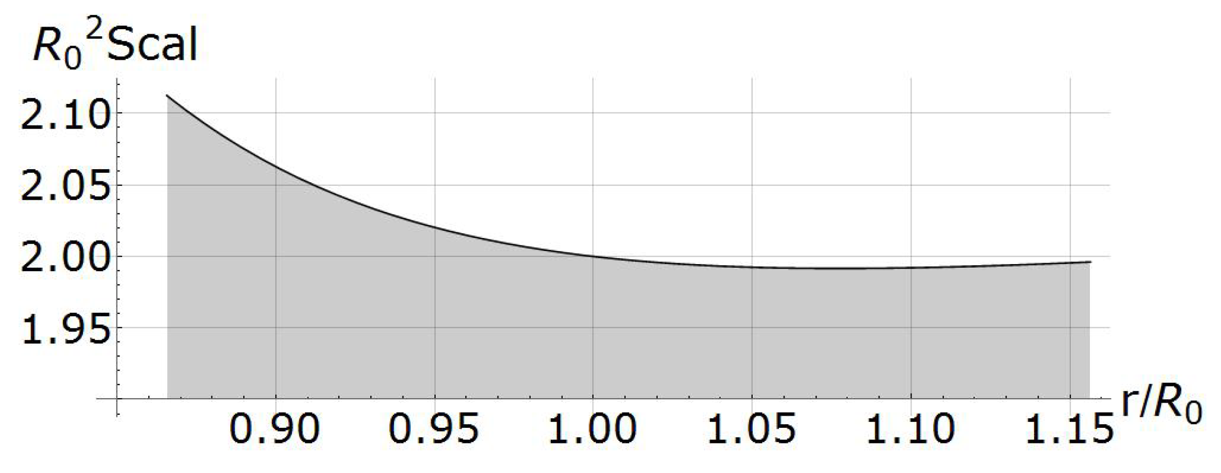
The first way for affine connection defining on $M_N$, lies in determining the Levi-Civita connection ${\nabla }^L$ obtained in the result of the synthesized material metric (34). For the problem in question the nonzero connection coefficients (26) with respect to $({\partial }_r,{\partial }_{\theta },{\partial }_{\phi })$ have the form:

$$\begin{array}{c}\mathrm{\Gamma }{}_{ 11}^1=-{\displaystyle \frac{A^{\prime }}{A}},\mathrm{\Gamma }{}_{ 22}^1={\displaystyle \frac{r{A}^2(r{a}^{\prime }-a)}{a^3}},\\ \mathrm{\Gamma }{}_{ 33}^1={\displaystyle \frac{r{A}^2{sin}^2\theta (r{a}^{\prime }-a)}{a^3}},\mathrm{\Gamma }{}_{ 12}^2=\mathrm{\Gamma }{}_{21}^2=\mathrm{\Gamma }{}_{ 13}^3=\mathrm{\Gamma }{}_{ 31}^3={\displaystyle \frac{1}{r}}-{\displaystyle \frac{a^{\prime }}{a}},\\ \mathrm{\Gamma }{}_{ 33}^2=-sin\theta cos\theta ,\mathrm{\Gamma }{}_{ 23}^3=\mathrm{\Gamma }{}_{ 32}^3=cot\theta .\end{array}$$

Corresponding scalar curvature (27) can be calculated as follows:

$$\mathrm{Scal}=2{\displaystyle \frac{-5r^2{A}^2{\left(a^{\prime }\right)}^2+2raA(rA{a}^{″}+a^{\prime }(r{A}^{\prime }+3A))-a^{2}A(2r{A}^{\prime }+A)+a^4}{r^2{a}^2}}.$$

(35)

The distribution for numerical values of scalar curvature (35), computed for data, used in Section 3, paragraph “Smoothing”, is shown on Figure 7.

As a result of such definition for peculiar (internal) geometry one can represent the reference non-Euclidean shape of the laminated body ${\tilde{\mathfrak{B}}}_N$ as Riemannian manifold ${\mathtt{S}}_R=(M_N,\mathsf{G},{\nabla }^L)$.

Another way for constructing connection on the manifold $M_N$ is related with the method of moving frame and Weitzenböck connection. Represent the field ${\mathsf{H}}^{-1}$, defined by (24), as ${\mathsf{H}}^{-1}=\left[{\mathsf{H}}^{-1}\right]{}_k^s{\partial }_s\otimes i^k$. Here $\left[{\mathsf{H}}^{-1}\right]{}_k^s$ are elements of the matrix defined as the product:

$$\left[{\mathsf{H}}^{-1}\right]=\mathrm{diag}(A,a,a).\left(\begin{array}{ccc}sin\theta cos\phi & sin\theta sin\phi & cos\theta \\ {\displaystyle \frac{1}{r}}cos\theta cos\phi & {\displaystyle \frac{1}{r}}cos\theta sin\phi & -{\displaystyle \frac{1}{r}}sin\theta \\ -{\displaystyle \frac{1}{rsin\theta }}sin\phi & {\displaystyle \frac{1}{rsin\theta }}cos\phi & 0\end{array}\right).$$

Introduce Weitzenböck connection ${\nabla }^W$ on $M_N$ as follows. According to (28), in the frame $({\partial }_r,{\partial }_{\theta },{\partial }_{\phi })$ one has:

$$\begin{array}{c}\mathrm{\Gamma }{}_{ 11}^1=-{\displaystyle \frac{A^{\prime }}{A}},\mathrm{\Gamma }{}_{ 22}^1=-{\displaystyle \frac{rA}{a}},\mathrm{\Gamma }{}_{ 33}^1=-{\displaystyle \frac{rA{sin}^2\theta }{a}},\\ \mathrm{\Gamma }{}_{ 12}^2=\mathrm{\Gamma }{}_{ 13}^3={\displaystyle \frac{1}{r}}-{\displaystyle \frac{a^{\prime }}{a}},\mathrm{\Gamma }{}_{ 21}^2=\mathrm{\Gamma }{}_{ 31}^3={\displaystyle \frac{a}{rA}},\\ \mathrm{\Gamma }{}_{ 33}^2=-sin\theta cos\theta ,\mathrm{\Gamma }{}_{ 23}^3=\mathrm{\Gamma }{}_{ 32}^3=cot\theta .\end{array}$$

With these connection coefficients one can construct non-Euclidean space ${\mathtt{S}}_R=(M_N,\mathsf{G},{\nabla }^W)$, which represents an alternative way for non-Euclidean stress-free shape definition. Torsion $\mathfrak{T}$ (29) of the connection ${\nabla }^W$ in coordinate frame is given below (only nonzero functions are shown):

$$\mathfrak{T}{}_{ 12}^2=\mathfrak{T}{}_{ 13}^3=-\mathfrak{T}{}_{ 21}^2=-\mathfrak{T}{}_{ 31}^3=-{\displaystyle \frac{a^{\prime }}{a}}-{\displaystyle \frac{a}{rA}}+{\displaystyle \frac{1}{r}}.$$

On Figure 8 the distribution of torsion tensor component $\mathfrak{T}{}_{ 12}^2$ is shown.

Interpretation of the dislocation density tensor. From the viewpoint of continual defects theory, Weitzenböck space $(M_N,\mathsf{G},{\nabla }^W)$ and Riemann space $(M_N,\mathsf{G},{\nabla }^L)$ represent solids with distributions of dislocations and disclinations, respectively, [30,34,67]. Torsion tensor $\mathfrak{T}$ is related with density of dislocations, while curvature tensor $\mathfrak{R}$ directly represents density of disclinations. For given torsion $\mathfrak{T}$ the dislocation density can be expressed equivalently as second rank tensor field $\aleph ={\aleph }^{ij}{\partial }_i\otimes {\partial }_j$, where [33]:

$${\aleph }^{ij}={\displaystyle \frac{1}{2}}\mathfrak{T}{}_m^{i}k{ϵ}^{jmk}.$$

(36)

Here $ϵ$ is Levi-Civita tensor with components

$${ϵ}^{ijk}={\displaystyle \frac{1}{\sqrt{\mathit{G}}}}{\mathit{e}}^{ijk},$$

where $\mathit{G}=det\left[{\mathit{G}}_{ij}\right]$ is determinant of material Riemannian metric $\mathsf{G}$ and ${\mathit{e}}^{ijk}$ is the alternator. The field ℵ defines Burgers vector $b=b^k{i}_k$,

$$b^i=\underset{\mathtt{S}}{\int }{\aleph }^{ij}{N}_{j}dA,$$

which complements contour in $\mathcal{E}$, formed by relaxed differential elements of $\partial \mathtt{S}$, into closed one. The integration is performed over two-dimensional submanifold $\mathtt{S}\subset {\mathtt{S}}_R$.

For the problem in question, the field ℵ (36) has the following dyadic decomposition:

$$\aleph =-{\displaystyle \frac{acsc\theta (a^2-Aa+rA{a}^{\prime })}{r^3}}\left\{{\partial }_{\theta }\otimes {\partial }_{\phi }-{\partial }_{\phi }\otimes {\partial }_{\theta }\right\}.$$

In order to give interpretation of the obtained field ℵ we recall that ${\tilde{\mathfrak{B}}}_N$ has laminated structure. This induces the laminated structure of the shape ${\mathtt{S}}_R$, that is,

$${\mathtt{S}}_R=\coprod _{\alpha \in \mathbb{I}}{\mathtt{L}}_{\alpha },$$

where ${\mathtt{L}}_{\alpha }={\varkappa }_R\left({\mathfrak{L}}_{\alpha }\right)$ are two-dimensional submanifolds of ${\mathtt{S}}_R$, the images of ${\mathfrak{L}}_{\alpha }$ under generalized reference configuration. The relaxation of each lamina ${\mathtt{L}}_{\alpha }$ to the stress-free state is governed by the field $\mathsf{H}$ (33).

To clarify the geometric meaning of the torsion on laminated structure consider one of laminae, say, ${\mathtt{L}}_{\alpha }$. For each its point $\mathtt{X}$ the tangent space ${\mathit{T}}_{\mathtt{X}}{\mathtt{L}}_{\alpha }$ is spanned over $({\partial }_{\theta }{|}_{\mathtt{X}},{\partial }_{\phi }{|}_{\mathtt{X}})$. The covector ${N|}_{\mathtt{X}}{=dr|}_{\mathtt{X}}$ annihilates this space, i.e., $N_{\mathtt{X}}\left({\mathit{T}}_{\mathtt{X}}{\mathtt{L}}_{\alpha }\right)=\left\{0\right\}$. Thus, $N=dr$ is field of annihilators for each vector space tangent to lamina. The direct consequence is that ${\aleph }^{mn}{N}_n={\aleph }^{m1}=0$. It means, that for each two-dimensional submanifold $\mathtt{S}$ that completely lies on some lamina ${\mathtt{L}}_{\alpha }$, the Burgers vector $b$ vanishes. This fact is the consequence of local compatibility: each lamina ${\mathtt{L}}_{\alpha }$ has stress-free shape. At the same time, if the manifold $\mathtt{S}$ passes through several laminae, the Burgers vector does not vanish. Indeed, there does not exist stress-free shape of $\mathtt{S}$. Note, that $\mathtt{S}$, in turn, is disjoint union of one-dimensional segments from laminae. Each such segment has stress-free shape.

5. Recovering of Local Deformation Field

Statement of the problem. It was shown in Section 4 that field of local deformations $\mathit{H}$ allows to synthesize non-Euclidean reference shape and, in particular, calculate geometric invariants of material connection ∇, which can be expressed in terms of incompatibility measures. If ∇ is Levi-Civita connection, then one can derive components of Ricci tensor, and if ∇ is Weitzenböck connection, then one can obtain components of dislocation density tensor. It is natural to consider the inverse problem, when one knows either curvature, or dislocation density tensor and is aimed at recovering of local deformation field.

To illustrate these derivations with application to central-symmetric laminated ball problem suppose that field $\mathit{H}$ is unknown, but the curvature or torsion for non-Euclidean stress-free shape are given. Keeping in mind the central antisymmetry one can take into account only scalar curvature and suppose that unknown family of locally stress-free shapes can be represented as continuous con-central family of balls. The reference shape (stressed intermediate shape) ${\mathcal{S}}_R$ can be one of them, or, perhaps, some other hollow ball with the same centre:

$${\mathcal{S}}_R=\{x\in \mathcal{E}|R^i<\parallel x-\mathcal{O}\parallel <R^{\mathit{e}}\},$$

where $R^i$ and $R^{\mathit{e}}$ are, respectively, internal and external radii, and $\mathcal{O}\in \mathcal{E}$ is the origin. Spherical coordinates $(r,\theta ,\phi )$ with origin at $\mathcal{O}$, related with Cartesian coordinates $(x^1,x^2,x^3)$ by formulae (3) are used. Values of spherical coordinates of points from ${\mathcal{S}}_R$ are denoted as $(R,\mathrm{\Theta },\mathrm{\Phi })$.

To obtain $\mathit{H}$ suppose that it is continuous and the following assumptions are valid:

(a)

For each value $\rho \in ]R^i,R^{\mathit{e}}[$ there exists a centrally-symmetric deformation ${\gamma }^{\left(\rho \right)}:{\mathcal{S}}_R\to {\mathcal{S}}^{\left(\rho \right)}$, such that the image ${\gamma }^{\left(\rho \right)}\left({\mathcal{L}}_{\rho }\right)$ of the sphere ${\mathcal{L}}_{\rho }=\{x\in \mathcal{E}|\parallel x-\mathcal{O}\parallel =\rho \}$ is stress-free (It means that the whole shape ${\mathcal{S}}^{\left(\rho \right)}={\gamma }^{\left(\rho \right)}\left({\mathcal{S}}_R\right)$ is globally self-stressed, while its subset, the sphere ${\gamma }^{\left(\rho \right)}\left({\mathcal{L}}_{\rho }\right)$, is stress-free, i.e., values of Cauchy stress-tensor vanish at its points).

(b)

In spherical coordinates $(R,\mathrm{\Theta },\mathrm{\Phi })$ the deformation ${\gamma }^{\left(\rho \right)}$ has the following representation (Note, that ${\gamma }^{\left(\rho \right)}$ is abstract map that transforms point of one shape to point of another shape, while ${\tilde{\gamma }}^{\left(\rho \right)}$ deals with tuples, i.e., it transforms triple of coordinates of point from reference shape to triple of coordinates of point from actual shape. If $\psi :\mathcal{E}\to {\mathbb{R}}^3$ denotes spherical coordinate map, then ${\tilde{\gamma }}^{\left(\rho \right)}=\psi \circ {\gamma }^{\left(\rho \right)}\circ {\psi }^{-1}{|}_{\psi \left({\mathcal{S}}_R\right)}$):

$${\tilde{\gamma }}^{\left(\rho \right)}(R,\mathrm{\Theta },\mathrm{\Phi })=\left(\omega \left(\rho \right)f_0\left(R\right),\mathrm{\Theta },\mathrm{\Phi }\right),$$

where $\omega :[R^i,R^{\mathit{e}}]\to {\mathbb{R}}_{>0}$ and $f_0:[R^i,R^{\mathit{e}}]\to {\mathbb{R}}_{>0}$ are smooth functions.

Function $\omega$ has to be determined from given curvature or torsion while function $f_0$ describes the deformation from reference to actual shapes embedded in Euclidean physical space. The latter can be obtained as the solution of conventional problem for hyperelastic solid.

Equations for $\omega$. Focus attention on the equations for $\omega$. For a fixed $\rho$ the deformation gradient (Recall that symbol D denotes derivative operation; see comment on page 8.) ${\mathit{K}}^{\left(\rho \right)}=D{\gamma }^{\left(\rho \right)}:{\mathcal{S}}_R\to \mathrm{Lin}(\mathcal{V};\mathcal{V})$ has the following dyadic representation:

$${\mathit{K}}^{\left(\rho \right)}{|}_{\mathcal{X}}=\omega \left(\rho \right)f_0^{\prime }\left(R\right){\mathit{e}}_r{|}_{{\gamma }^{\left(\rho \right)}\left(\mathcal{X}\right)}\otimes {\mathit{e}}^r{|}_{\mathcal{X}}+{\mathit{e}}_{\theta }{|}_{{\gamma }^{\left(\rho \right)}\left(\mathcal{X}\right)}\otimes {\mathit{e}}^{\theta }{|}_{\mathcal{X}}+{\mathit{e}}_{\phi }{{|}_{{\gamma }^{\left(\rho \right)}\left(\mathcal{X}\right)}\otimes {\mathit{e}}^{\phi }|}_{\mathcal{X}}.$$

Here $({\mathit{e}}_r,{\mathit{e}}_{\theta },{\mathit{e}}_{\phi })$ is field of local bases that corresponds to spherical coordinates $(r,\theta ,\phi )$ and $({\mathit{e}}^r,{\mathit{e}}^{\theta },{\mathit{e}}^{\phi })$ is field of dual bases. For every point $\mathcal{X}\in {\mathcal{L}}_{\rho }$ the linear mapping ${\mathit{K}}^{\left(\rho \right)}{|}_{\mathcal{X}}:\mathcal{V}\to \mathcal{V}$ transforms stressed infinitesimal neighborhood of $\mathcal{X}$ into infinitesimal stress-free neighborhood of point ${\gamma }^{\left(\rho \right)}\left(\mathcal{X}\right)$.

In the dyadic representation of ${\mathit{K}}^{\left(\rho \right)}{|}_{\mathcal{X}}$ the left “leg” of ${\mathit{e}}_i{{|}_{{\gamma }^{\left(\rho \right)}\left(\mathcal{X}\right)}\otimes {\mathit{e}}^j|}_{\mathcal{X}}$ is defined on point from intermediate shape, while the right “leg” is defined on point from reference one. Since both “legs” are vectors from one and the same translation space $\mathcal{V}$, one can use tilt [40] to define them on reference shape ${\mathcal{S}}_R$. Indeed, the following formulae hold:

$${\mathit{e}}_r{|}_{{\gamma }^{\left(\rho \right)}\left(\mathcal{X}\right)}={\mathit{e}}_r{|}_{\mathcal{X}},{\mathit{e}}_{\theta }{|}_{{\gamma }^{\left(\rho \right)}\left(\mathcal{X}\right)}=\omega \left(\rho \right)\frac{f_0\left(R\right)}{R}{\mathit{e}}_{\theta }{|}_{\mathcal{X}},{\mathit{e}}_{\phi }{{|}_{{\gamma }^{\left(\rho \right)}\left(\mathcal{X}\right)}=\omega \left(\rho \right)\frac{f_0\left(R\right)}{R}{\mathit{e}}_{\phi }|}_{\mathcal{X}}.$$

Then, it follows that:

$${\mathit{K}}^{\left(\rho \right)}{|}_{\mathcal{X}}=\omega \left(\rho \right)f_0^{\prime }\left(R\right){\mathit{e}}_r{{|}_{\mathcal{X}}\otimes {\mathit{e}}^r|}_{\mathcal{X}}+\omega \left(\rho \right){\displaystyle \frac{f_0\left(R\right)}{R}}\left({\mathit{e}}_{\theta }{|}_{\mathcal{X}}\otimes {\mathit{e}}^{\theta }{|}_{\mathcal{X}}+{\mathit{e}}_{\phi }{{|}_{\mathcal{X}}\otimes {\mathit{e}}^{\phi }|}_{\mathcal{X}}\right).$$

(37)

Thus, to each sphere ${\mathcal{L}}_{\rho }$ there corresponds local deformation ${\mathit{K}}^{\left(\rho \right)}$, generated by global deformation ${\gamma }^{\left(\rho \right)}$. The field of local deformations $\mathit{H}:{\mathcal{S}}_R\to \mathrm{Lin}(\mathcal{V};\mathcal{V})$ is synthesized upon family ${\left\{{\mathit{K}}^{\left(\rho \right)}\right\}}_{\rho \in ]R^i,R^{\mathit{e}}[}$ of deformation gradients (37) as follows:

$$\mathit{H}\left(\rho \right):={\mathit{K}}^{\left(\rho \right)}{|}_{R=\rho }.$$

Now, it is convenient to replace all occurrences of symbol $\rho$ by R. Since $f_0$ does not contain variable $\rho$, the functional dependence would not be changed. Thus, one arrives at the following dyadic decomposition:

$${\mathit{H}|}_{\mathcal{X}}=\omega \left(R\right)f_0^{\prime }\left(R\right){\mathit{e}}_r{{|}_{\mathcal{X}}\otimes {\mathit{e}}^r|}_{\mathcal{X}}+\omega \left(R\right){\displaystyle \frac{f_0\left(R\right)}{R}}\left({\mathit{e}}_{\theta }{|}_{\mathcal{X}}\otimes {\mathit{e}}^{\theta }{|}_{\mathcal{X}}+{\mathit{e}}_{\phi }{{|}_{\mathcal{X}}\otimes {\mathit{e}}^{\phi }|}_{\mathcal{X}}\right).$$

(38)

As it was discussed above, $M_R$ denotes underlying manifold of the shape ${\mathcal{S}}_R$, i.e., it is the structure, obtained upon the shape ${\mathcal{S}}_R$ by erasing Euclidean geometry from it.

Material metric $\mathsf{G}$ on $M_R$, that corresponds to tensor field (38), can be obtained via the general relation (25). Its dyadic representation has the form:

$$\begin{array}{c}\mathsf{G}={\left[\omega \left(R\right)f_0^{\prime }\left(R\right)\right]}^{2}dR\otimes dR+{\left[\omega \left(R\right)f_0\left(R\right)\right]}^{2}d\mathrm{\Theta }\otimes d\mathrm{\Theta }+\hfill \\ \hfill +{[\omega \left(R\right)f_0\left(R\right)sin\mathrm{\Theta }]}^{2}d\mathrm{\Phi }\otimes d\mathrm{\Phi }.\end{array}$$

(39)

Here $(dR,d\mathrm{\Theta },d\mathrm{\Phi })$ is coordinate coframe, dual to coordinate frame $({\partial }_R,{\partial }_{\mathrm{\Theta }},{\partial }_{\mathrm{\Phi }})$ generated by coordinates $(R,\mathrm{\Theta },\mathrm{\Phi })$.

Recall that $\omega$ is still unknown. To obtain equation with respect to $\omega$ one can use the expression for Levi-Civita connection ${\nabla }^L$ on manifold $M_R$ that is related with Riemannian metric (39). Nonzero connection coefficients (26) with respect to coordinates $(R,\mathrm{\Theta },\mathrm{\Phi })$ have the form:

$$\begin{array}{c}\mathrm{\Gamma }{}_{ 11}^1={\displaystyle \frac{f_0^{\prime \prime }}{f_0^{\prime }}}+{\displaystyle \frac{{\omega }^{\prime }}{\omega }},\mathrm{\Gamma }{}_{ 22}^1=-{\displaystyle \frac{f_0(\omega f_0^{\prime }+f_0{\omega }^{\prime })}{\omega {\left[f_0^{\prime }\right]}^2}},\\ \mathrm{\Gamma }{}_{ 33}^1=-{\displaystyle \frac{f_0{sin}^2\mathrm{\Theta }(\omega f_0^{\prime }+f_0{\omega }^{\prime })}{\omega {\left[f_0^{\prime }\right]}^2}},\mathrm{\Gamma }{}_{ 12}^2=\mathrm{\Gamma }{}_{ 21}^2=\mathrm{\Gamma }{}_{ 13}^3=\mathrm{\Gamma }{}_{ 31}^3={\displaystyle \frac{f_0^{\prime }}{f_0}}+{\displaystyle \frac{{\omega }^{\prime }}{\omega }},\\ \mathrm{\Gamma }{}_{ 33}^2=-sin\mathrm{\Theta }cos\mathrm{\Theta },\mathrm{\Gamma }{}_{ 23}^3=\mathrm{\Gamma }{}_{ 32}^3=cot\mathrm{\Theta }.\end{array}$$

Thus, one obtains the following expression for scalar curvature (27):

$$\mathrm{Scal}={\displaystyle \frac{2f_0{f}_0^{\prime }{\left[{\omega }^{\prime }\right]}^2-4\omega (f_0{f}_0^{\prime }{\omega }^{″}+{\omega }^{\prime }(2{\left[f_0^{\prime }\right]}^2-f_0{f}_0^{″}))}{f_0{\omega }^4{\left[f_0^{\prime }\right]}^3}}.$$

(40)

For given scalar curvature (or, equivalently, the density of disclinations) one can treat the (40) as the equation with respect to $\omega$. Together with the momentum equation with respect to $f_0$ one obtains complete system of equations, which solution determines $\mathit{H}$ with respect to arbitrary chosen intermediate shape and its deformation into actual shape, balanced with given external fields.

A slightly different equation arises if Weitzenböck connection ${\nabla }^W$ is introduced on $M_R$. According to (28), in the frame $({\partial }_R,{\partial }_{\mathrm{\Theta }},{\partial }_{\mathrm{\Phi }})$ one has:

$$\begin{array}{c}\mathrm{\Gamma }{}_{ 11}^{1}1={\displaystyle \frac{f_0^{″}}{f_0^{\prime }}}+{\displaystyle \frac{{\omega }^{\prime }}{\omega }},\mathrm{\Gamma }{}_{ 22}^1=-{\displaystyle \frac{f_0}{f_0^{\prime }}},\\ \mathrm{\Gamma }{}_{ 33}^1=-{\displaystyle \frac{f_0{sin}^2\mathrm{\Theta }}{f_0^{\prime }}},\mathrm{\Gamma }{}_{ 12}^2=\mathrm{\Gamma }{}_{ 13}^3={\displaystyle \frac{f_0^{\prime }}{f_0}}+{\displaystyle \frac{{\omega }^{\prime }}{\omega }},\mathrm{\Gamma }{}_{ 21}^2=\mathrm{\Gamma }{}_{ 31}^3={\displaystyle \frac{f_0^{\prime }}{f_0}},\\ \mathrm{\Gamma }{}_{ 33}^2=-sin\mathrm{\Theta }cos\mathrm{\Theta },\mathrm{\Gamma }{}_{ 23}^3=\mathrm{\Gamma }{}_{ 32}^3=cot\mathrm{\Theta }.\end{array}$$

Components (29) of torsion tensor $\mathfrak{T}$ of the connection ${\nabla }^W$ in coordinate frame are given below (only nonzero functions are shown):

$$\mathfrak{T}{}_{ 12}^2=\mathfrak{T}{}_{ 13}^3=-\mathfrak{T}{}_{ 21}^2=-\mathfrak{T}{}_{ 31}^3={\displaystyle \frac{{\omega }^{\prime }}{\omega }}.$$

It may seem desirable to use torsion tensor as field, upon which one can obtain the distribution of reference shapes expressed in terms of function $\omega$. Meanwhile, torsion tensor is not suitable for this purpose since it does not contain any metric information. By this reason, we use dislocation density tensor with components (36), that contains metric in its definition. Taking into account the expression (39) for metric, one gets:

$$\aleph ={\displaystyle \frac{{\omega }^{\prime }}{f_0^2{\omega }^4{f}_0^{\prime }sin\mathrm{\Theta }}}\left\{{\partial }_{\mathrm{\Theta }}\otimes {\partial }_{\mathrm{\Phi }}-{\partial }_{\mathrm{\Phi }}\otimes {\partial }_{\mathrm{\Theta }}\right\}.$$

(41)

Again, for the given ℵ (the density of dislocations) one can treat the relation (41) as the equation with respect to unknown $\omega$ and $f_0$. Complementing this equation with the impulse balance equation, one obtains two equations with respect to two unknowns. The solution of this system, corresponding to suitable boundary conditions, determines the field $\mathit{H}$ and compatible deformations that bring intermediate shape into actual one.

6. Conclusions

The above discussion makes it clear that the global stress-free shape of the body, produced with some additive process, can be found on a smooth manifold endowed with non-Euclidean affine connection, which turns it into non-Euclidean space, for instance, into Riemannian or Weitzenböck spaces. At the same time, the non-Euclidean geometry become a valid alternative to geometrical relations adopted nowadays in non-linear theory of distributed defects [32,33,34]. Although in the framework of this theory the density of defects, or, similarly, the explicit form of material connection, is considered to be predefined. In this regard, it seems to be natural to interpret the final body with non-Euclidean material connection, obtained by smoothing procedure, described above, as the elastic body with some predefined distribution of defects. It enables to encode specific mechanical features, related either with self-stressed structure of additively produced bodies, or, in other terms, with nonholonomy of local reference configuration, or, ultimately, with specific material connection in a manner, customary in non-linear theory of distributed defects.

References

- Gibson, I.; Rosen, D.; Stucker, B. Additive Manufacturing Technologies: 3D Printing, Rapid Prototyping, and Direct Digital Manufacturing; Springer: New York, NY, USA, 2015. [Google Scholar] [CrossRef]
- Gu, D. Laser Additive Manufacturing of High-Performance Materials; Springer: Berlin/Heidelberg, Germany, 2015. [Google Scholar] [CrossRef]
- Bártolo, P.J. (Ed.) Stereolithography: Materials, Processes and Applications; Springer: New York, NY, USA, 2011. [Google Scholar] [CrossRef]
- Devine, D.M. (Ed.) Polymer-Based Additive Manufacturing: Biomedical Applications; Springer International Publishing: Berlin/Heidelberg, Germany, 2019. [Google Scholar] [CrossRef]
- Kumar, S. Additive Manufacturing Processes; Springer International Publishing: Berlin/Heidelberg, Germany, 2020. [Google Scholar] [CrossRef]
- Bertini, L.; Bucchi, F.; Frendo, F.; Moda, M.; Monelli, B.D. Residual stress prediction in selective laser melting. Int. J. Adv. Manuf. Technol. 2019, 105, 609–636. [Google Scholar] [CrossRef]
- Huang, Q.; Zhang, J.; Sabbaghi, A.; Dasgupta, T. Optimal offline compensation of shape shrinkage for three-dimensional printing processes. IIE Trans. 2015, 47, 431–441. [Google Scholar] [CrossRef]
- Mughal, M.; Fawad, H.; Mufti, R. Finite element prediction of thermal stresses and deformations in layered manufacturing of metallic parts. Acta Mech. 2006, 183, 61–79. [Google Scholar] [CrossRef]
- Mukherjee, T.; Zhang, W.; DebRoy, T. An improved prediction of residual stresses and distortion in additive manufacturing. Comput. Mater. Sci. 2017, 126, 360–372. [Google Scholar] [CrossRef] [Green Version]
- Mishurova, T.; Artzt, K.; Haubrich, J.; Requena, G.; Bruno, G. New aspects about the search for the most relevant parameters optimizing SLM materials. Addit. Manuf. 2019, 25, 325–334. [Google Scholar] [CrossRef]
- Parry, L.; Ashcroft, I.; Wildman, R. Geometrical effects on residual stress in selective laser melting. Addit. Manuf. 2019, 25, 166–175. [Google Scholar] [CrossRef]
- Vastola, G.; Zhang, G.; Pei, Q.; Zhang, Y.W. Controlling of residual stress in additive manufacturing of Ti6Al4V by finite element modeling. Addit. Manuf. 2016, 12, 231–239. [Google Scholar] [CrossRef]
- Southwell, R. An Introduction to the Theory of Elasticity for Engineers and Physicists; Oxford Engineering Science Series; Oxford University Press: Oxford, UK, 1941. [Google Scholar]
- Brown, C.B.; Goodman, L.E.; Jeffreys, H. Gravitational stresses in accreted bodies. Proc. R. Soc. Lond. Ser. A Math. Phys. Sci. 1963, 276, 571–576. [Google Scholar] [CrossRef]
- Arutyunyan, N.; Drozdov, A.; Naumov, V. Mechanics of Growing Viscoelastoplastic Solids; Nauka Press: Moscow, Russia, 1987. (In Russian) [Google Scholar]
- Metlov, V.V. On the accretion of inhomogeneous viscoelastic bodies at finite strains. Appl. Math. Mech. 1985, 49, 637–647. [Google Scholar]
- Zurlo, G.; Truskinovsky, L. Printing Non-Euclidean Solids. Phys. Rev. Lett. 2017, 119, 048001. [Google Scholar] [CrossRef] [Green Version]
- Zurlo, G.; Truskinovsky, L. Inelastic surface growth. Mech. Res. Commun. 2018, 93, 174–179. [Google Scholar] [CrossRef] [Green Version]
- Lychev, S.; Manzhirov, A. The mathematical theory of growing bodies. Finite deformations. J. Appl. Math. Mech. 2013, 77, 421–432. [Google Scholar] [CrossRef]
- Truskinovsky, L.; Zurlo, G. Nonlinear elasticity of incompatible surface growth. Phys. Rev. E 2019, 99, 053001. [Google Scholar] [CrossRef] [Green Version]
- Sozio, F.; Yavari, A. Nonlinear mechanics of accretion. J. Nonlinear Sci. 2019, 29, 1813–1863. [Google Scholar] [CrossRef]
- Sozio, F.; Yavari, A. Nonlinear mechanics of surface growth for cylindrical and spherical elastic bodies. J. Mech. Phys. Solids 2017, 98, 12–48. [Google Scholar] [CrossRef] [Green Version]
- Lychev, S.; Koifman, K. Nonlinear evolutionary problem for a laminated inhomogeneous spherical shell. Acta Mech. 2019, 230, 3989–4020. [Google Scholar] [CrossRef]
- Lychev, S.A.; Kostin, G.V.; Lycheva, T.N.; Koifman, K.G. Non-Euclidean Geometry and Defected Structure for Bodies with Variable Material Composition. J. Phys. Conf. Ser. 2019, 1250, 012035. [Google Scholar] [CrossRef]
- Epstein, M.; Elzanowski, M. Material Inhomogeneities and Their Evolution: A Geometric Approach; Springer Science & Business Media: Berlin/Heidelberg, Germany, 2007. [Google Scholar]
- Epstein, M. The Geometrical Language of Continuum Mechanics; Cambridge University Press: Cambridge, UK, 2010. [Google Scholar]
- Lychev, S.; Koifman, K. Geometry of Incompatible Deformations: Differential Geometry in Continuum Mechanics; De Gruyter: Berlin, Germany, 2018. [Google Scholar]
- Kupferman, R.; Olami, E.; Segev, R. Continuum Dynamics on Manifolds: Application to Elasticity of Residually-Stressed Bodies. J. Elast. 2017, 128, 61–84. [Google Scholar] [CrossRef] [Green Version]
- Segev, R.; Epstein, M. (Eds.) Geometric Continuum Mechanics; Birkhäuser: Basel, Switzerland, 2020. [Google Scholar] [CrossRef]
- Kröner, E. Allgemeine Kontinuumstheorie der Versetzungen und Eigenspannungen. Arch. Ration. Mech. Anal. 1959, 4, 18–334. [Google Scholar] [CrossRef]
- De Wit, R. Fundamental Aspects of Dislocation Theory; Chapter Linear theory of Static Disclinations; National Bureau of Standards (U.S.): Gaithersburg, MD, USA, 1970; Volume I, pp. 651–673. [Google Scholar]
- Yavari, A.; Goriely, A. Weyl geometry and the nonlinear mechanics of distributed point defects. Proc. R. Soc. A 2012, 468, 3902–3922. [Google Scholar] [CrossRef] [Green Version]
- Yavari, A.; Goriely, A. Riemann–Cartan Geometry of Nonlinear Dislocation Mechanics. Arch. Ration. Mech. Anal. 2012, 205, 59–118. [Google Scholar] [CrossRef]
- Miri, M.; Rivier, N. Continuum elasticity with topological defects, including dislocations and extra-matter. J. Phys. Math. Gen. 2002, 35, 1727–1739. [Google Scholar] [CrossRef]
- Epstein, M.; Segev, R. On the Geometry and Kinematics of Smoothly Distributed and Singular Defects. In Differential Geometry and Continuum Mechanics; Chen, G.Q.G., Grinfeld, M., Knops, R.J., Eds.; Springer International Publishing: Berlin/Heidelberg, Germany, 2015; pp. 203–234. [Google Scholar] [CrossRef] [Green Version]
- Abraham, R.; Marsden, J.E.; Ratiu, T. Manifolds, Tensor Analysis, and Applications; Springer Science & Business Media: Berlin/Heidelberg, Germany, 2012; Volume 75. [Google Scholar]
- Lee, J.M. Introduction to Smooth Manifolds; Springer: New York, NY, USA, 2012. [Google Scholar] [CrossRef]
- Noll, W. Materially uniform simple bodies with inhomogeneities. Arch. Ration. Mech. Anal. 1967, 27, 1–32. [Google Scholar] [CrossRef]
- Wang, C.C. On the geometric structures of simple bodies, a mathematical foundation for the theory of continuous distributions of dislocations. Arch. Ration. Mech. Anal. 1967, 27, 33–94. [Google Scholar] [CrossRef]
- Marsden, J.E.; Hughes, T.J. Mathematical Foundations of Elasticity; Courier Corporation: Chelmsford, MA, USA, 1994. [Google Scholar]
- Segev, R.; Rodnay, G. Cauchy’s Theorem on Manifolds. J. Elast. 1999, 56, 129–144. [Google Scholar] [CrossRef]
- Kanso, E.; Arroyo, M.; Tong, Y.; Yavari, A.; Marsden, J.G.; Desbrun, M. On the geometric character of stress in continuum mechanics. Z. Angew. Math. Phys. 2007, 58, 843–856. [Google Scholar] [CrossRef] [Green Version]
- Segev, R.; Falach, L. Velocities, Stresses and Vector Bundle Valued Chains. J. Elast. 2011, 105, 187–206. [Google Scholar] [CrossRef]
- Romano, G.; Barretta, R.; Diaco, M. Geometric continuum mechanics. Meccanica 2014, 49, 111–133. [Google Scholar] [CrossRef]
- Segev, R. Continuum mechanics, stresses, currents and electrodynamics. Philos. Trans. R. Soc. A Math. Phys. Eng. Sci. 2016, 374, 20150174. [Google Scholar] [CrossRef]
- Roychowdhury, A.; Gupta, A. Non-metric connection and metric anomalies in materially uniform elastic solids. arXiv 2016, arXiv:1601.06905. [Google Scholar] [CrossRef] [Green Version]
- Burger, D. Sphereland: A Fantasy About Curved Spaces and an Expanding Universe; Barnes & Noble: Wheaton, IL, USA, 1983. [Google Scholar]
- Wang, C.C. Universal solutions for incompressible laminated bodies. Arch. Ration. Mech. Anal. 1968, 29, 161–192. [Google Scholar] [CrossRef]
- Polyanin, A.D. Generalized traveling-wave solutions of nonlinear reaction–diffusion equations with delay and variable coefficients. Appl. Math. Lett. 2019, 90, 49–53. [Google Scholar] [CrossRef]
- Sorokin, V.G.; Polyanin, A.D. Nonlinear partial differential equations with delay: Linear stability/instability of solutions, numerical integration. J. Phys. Conf. Ser. 2019, 1205, 012053. [Google Scholar] [CrossRef]
- Weyl, H. Space, Time, Matter; Dover Publications Inc.: Mignola, NY, USA, 1952. [Google Scholar]
- Truesdell, C.; Noll, W. The Non-Linear Field Theories of Mechanics/Die Nicht-Linearen Feldtheorien der Mechanik; Springer Science & Business Media: Berlin/Heidelberg, Germany, 2013; Volume 2. [Google Scholar]
- Rivlin, R. Large elastic deformations of isotropic materials, I Fundamental concepts. Philos. Trans. R. Soc. Lond. Ser. A Math. Phys. Sci. 1948, 240, 459–490. [Google Scholar]
- Kukudzhanov, V. Numerical Continuum Mechanics; De Gruyter: Berlin, Germany, 2013. [Google Scholar]
- Hardy, G.H. Weierstrass’s nondifferentiable function. Trans. Am. Math. Soc. 1916, 17, 301–325. [Google Scholar] [CrossRef]
- Husemoller, D. Fibre Bundles; Springer: New York, NY, USA, 1994. [Google Scholar] [CrossRef]
- Lee, J.M. Introduction to Topological Manifolds; Springer: New York, NY, USA, 2011. [Google Scholar] [CrossRef]
- Lychev, S.; Koifman, K. Material Affine Connections for Growing Solids. Lobachevskii J. Math. 2020, 41, 2034–2052. [Google Scholar] [CrossRef]
- Lychev, S.; Koifman, K. Contorsion of Material Connection in Growing Solids. Lobachevskii J. Math. 2021, 42, 1852–1875. [Google Scholar] [CrossRef]
- Lee, J.M. Introduction to Riemannian Manifolds; Springer: Cham, Switzerland, 2018. [Google Scholar] [CrossRef]
- Lurie, A.I. Non-Linear Theory of Elasticity; Elsevier: Amsterdam, The Netherlands, 2012. [Google Scholar]
- Cartan, E.J. Sur les variétés á connexion affine et la théorie de la relativité généralisée. Annales Scientifiques de l’Ecole Normale Supérieure 1923, 40, 325–412. [Google Scholar] [CrossRef]
- Goldberg, V.; Chern, S.S. Riemannian Geometry in an Orthogonal Frame; World Scientific Publishing Company: Singapore, 2001. [Google Scholar]
- Fernandez, O.E.; Bloch, A.M. The Weitzenböck Connection and Time Reparameterization in Nonholonomic Mechanics. J. Math. Phys. 2011, 52, 012901. [Google Scholar] [CrossRef] [Green Version]
- Maugin, G.A. Material Inhomogeneities in Elasticity; CRC Press: Boca Raton, FL, USA, 1993; Volume 3. [Google Scholar]
- Lee, E.H. Elastic-Plastic Deformation at Finite Strains. J. Appl. Mech. 1969, 36, 1–6. [Google Scholar] [CrossRef]
- Grachev, A.; Nesterov, A.; Ovchinnikov, S. The Gauge Theory of Point Defects. Phys. Status Solidi B Basic Solid State Phys. 1989, 156, 403–410. [Google Scholar] [CrossRef]
Figure 1.
Layers and Assemblies.
Figure 2.
Locally stress-free shapes.
Figure 3.
Stress distributions for an assembly of 5 layers.
Figure 4.
Stress distributions for an assembly of 20 layers.
Figure 5.
Rendering self-intersecting reference shapes.
Figure 6.
Distortion parameters for continuous and discrete assemblies.
Figure 7.
Scalar curvature for data, given in Section 3.
Figure 8.
Torsion tensor component for data, given in Section 3.
Publisher’s Note: MDPI stays neutral with regard to jurisdictional claims in published maps and institutional affiliations. |
© 2021 by the authors. Licensee MDPI, Basel, Switzerland. This article is an open access article distributed under the terms and conditions of the Creative Commons Attribution (CC BY) license (https://creativecommons.org/licenses/by/4.0/).
Share and Cite
MDPI and ACS Style
Lychev, S.; Koifman, K.; Djuzhev, N. Incompatible Deformations in Additively Fabricated Solids: Discrete and Continuous Approaches. Symmetry 2021, 13, 2331. https://doi.org/10.3390/sym13122331
AMA Style
Lychev S, Koifman K, Djuzhev N. Incompatible Deformations in Additively Fabricated Solids: Discrete and Continuous Approaches. Symmetry. 2021; 13(12):2331. https://doi.org/10.3390/sym13122331
Chicago/Turabian StyleLychev, Sergey, Konstantin Koifman, and Nikolay Djuzhev. 2021. "Incompatible Deformations in Additively Fabricated Solids: Discrete and Continuous Approaches" Symmetry 13, no. 12: 2331. https://doi.org/10.3390/sym13122331
Note that from the first issue of 2016, this journal uses article numbers instead of page numbers. See further details here.