A Fractional Approach to a Computational Eco-Epidemiological Model with Holling Type-II Functional Response

Abstract

Eco-epidemiological can be considered as a significant combination of two research fields of computational biology and epidemiology. These problems mainly take ecological systems into account of the impact of epidemiological factors. In this paper, we examine the chaotic nature of a computational system related to the spread of disease into a specific environment involving a novel differential operator called the Atangana–Baleanu fractional derivative. To approximate the solutions of this fractional system, an efficient numerical method is adopted. The numerical method is an implicit approximate method that can provide very suitable numerical approximations for fractional problems due to symmetry. Symmetry is one of the distinguishing features of this technique compared to other methods in the literature. Through considering different choices of parameters in the model, several meaningful numerical simulations are presented. It is clear that hiring a new derivative operator greatly increases the flexibility of the model in describing the different scenarios in the model. The results of this paper can be very useful help for decision-makers to describe the situation related to the problem, in a more efficient way, and control the epidemic.

1. Introduction

Nature is full of interactions between different species of living beings to provide food, shelter, and other essential needs. In many cases, it is necessary to gain a better understanding of these interactions to preserve different species of living organisms in nature. In recent years, the use of mathematical modeling in the study of problems in computational biology has attracted the attention of many experts in the fields of mathematics and biology [1,2,3,4,5,6,7,8,9,10,11,12,13]. As a result, and based on these important applications, many effective techniques have been proposed in solving mathematical models arising from such problems [14,15,16,17,18,19,20,21,22,23,24,25,26,27,28,29,30,31,32,33,34,35,36,37,38,39]. One of the most interesting aspects of such problems is examining cases where the environment has been affected by an infectious disease. Such models are referred to as eco-epidemiological models and have also been explored with an aim of disease control. Certainly, in this case, the spread of disease among the populations considered in the model can have a direct impact on the survival or extinction of species in the problem.

Nowadays, with the spread of infectious and contagious diseases throughout the natural world and their direct impact on food interactions in ecosystems, many models have been presented and studied. For example, taking the weak Allee effect and harvesting in prey population into account, the following nonlinear delay system of equations has been proposed [40]:

$$\begin{array}{c}\frac{d\mathsf{S}\left(t\right)}{dt}=\mathsf{S}\left(t\right)\left[(1-\mathsf{S}\left(t\right)-\mathsf{I}\left(t\right))\frac{\mathsf{S}\left(t\right)}{\mathsf{S}\left(t\right)+\theta }-\beta \mathsf{I}\left(t\right)-q_{1}E\right],\hfill \\ \frac{d\mathsf{I}\left(t\right)}{dt}=\mathsf{I}\left(t\right)[\beta \mathsf{S}\left(t\right)-a\mathsf{P}\left(t\right)-\mu -q_{2}E,\hfill \\ \frac{d\mathsf{P}\left(t\right)}{dt}=\alpha \mathsf{P}(t-\tau )\mathsf{I}(t-\tau )-d\mathsf{P}\left(t\right),\hfill \end{array}$$

(1)

where existing parameters in the model are introduced in Reference [40].

Furthermore, an eco-epidemiological model has been investigated in [41] under the combined influence of strong-Allee parameter and competition coefficients, given by

$$\begin{array}{c}\frac{d\mathsf{S}\left(t\right)}{dt}=\left[r-b\mathsf{S}\left(t\right)-c\mathsf{I}\left(t\right)\right]\mathsf{S}\left(t\right)\left(1-\frac{\theta +f}{\mathsf{S}\left(t\right)+f}\right)-\frac{\beta \mathsf{I}\left(t\right)\mathsf{S}\left(t\right)}{a+\mathsf{S}\left(t\right)},\hfill \\ \frac{d\mathsf{I}\left(t\right)}{dt}=\frac{\beta \mathsf{I}\left(t\right)\mathsf{S}\left(t\right)}{a+\mathsf{S}\left(t\right)}-\frac{{\alpha }_1\mathsf{I}\left(t\right)\mathsf{P}\left(t\right)}{d+\mathsf{I}\left(t\right)}-\mu \mathsf{I}\left(t\right),\hfill \\ \frac{d\mathsf{P}\left(t\right)}{dt}=\frac{{\gamma }_1\mathsf{I}\left(t\right)\mathsf{P}\left(t\right)}{d+\mathsf{I}\left(t\right)}-m\mathsf{P}\left(t\right).\hfill \end{array}$$

(2)

To get some more information about existing parameters in Model (2), please refer to the work in [41].

The authors of [42] have considered that an infectious disease has spread to the prey and predator populations in the environment. In their work, they have used the following nonlinear system to describe these interactions:

$$\begin{array}{c}\frac{d\mathsf{S}\left(t\right)}{dt}=\left[r-b\mathsf{S}\left(t\right)-c\mathsf{I}\left(t\right)-\frac{\beta \mathsf{I}\left(t\right)}{a+\mathsf{S}\left(t\right)}-\frac{{\alpha }_1\mathsf{P}\left(t\right)}{e+\mathsf{S}\left(t\right)}\right]\mathsf{S}\left(t\right),\hfill \\ \frac{d\mathsf{I}\left(t\right)}{dt}=\left[\frac{\beta \mathsf{S}\left(t\right)}{a+\mathsf{S}\left(t\right)}-\frac{{\alpha }_2\mathsf{P}\left(t\right)}{d+\mathsf{I}\left(t\right)}-\mu \right]\mathsf{I}\left(t\right),\hfill \\ \frac{d\mathsf{P}\left(t\right)}{dt}=\left[\left(\frac{c_1{\alpha }_1\mathsf{S}\left(t\right)}{e+\mathsf{S}\left(t\right)}+\frac{c_2{\alpha }_2\mathsf{I}\left(t\right)}{d+\mathsf{I}\left(t\right)}\right)\frac{\mathsf{P}\left(t\right)}{\theta +\mathsf{P}\left(t\right)}-m\right]\mathsf{P}\left(t\right).\hfill \end{array}$$

(3)

In all these models, $\mathsf{S}\left(t\right)$ and $\mathsf{I}\left(t\right)$ denote the susceptible and the diseased prey, respectively. Further, $\mathsf{P}\left(t\right)$ has been employed to describe the predator population. More explanations about existing parameters in Model (3) can be found in [42].

In recent years, the use of fractional derivative operators in the modeling various problems in mathematics, physics, and engineering has increased significantly. For example, In [43], a SIR epidemic model with Crowley–Martin type functional response and Holling type-II treatment rate is investigated. Moreover, a comparison based on newly defined fractional derivative operators which are called as Caputo–Fabrizio (CF) and Atangana–Baleanu (AB) has been presented in [44]. A model for HIV-1 primary infection with treatment in fractional order along with its Global dynamics is considered in [45]. The FitzHugh–Nagumo (F–N) model has been studied in [46] using the nerve impulses process. In [47], several chaotic systems, involving Atangana–Baleanu fractional derivative operator with interesting behaviors are presented. In [48], a fractal-fractional differentiation for the modeling and mathematical analysis of nonlinear diarrhea transmission dynamics under the use of real data has been investigated. In [49], hybrid mathematical models of new strains and co-infection in Caputo, Caputo–Fabrizio, and Atangana–Baleanu are studied. Further, a mathematical model in describing the transmission of Nipah virus within a targeted population has been proposed in [50], More examples can be found in [13,23,51,52,53,54,55,56,57,58,59,60,61,62,63,64,65].

One of the main reasons for this increase in popularity is perhaps the fact that these operators are equipped with the concept of memory. In fact, to determine the value of the derivative in these fractional operators, it is necessary to collect all the previous information of those phenomena in the calculations from the beginning to that specific time situation. This valuable feature of operators plays a very vital and influential role in biological modeling, where the current behavior of the variables in the models is very much influenced by their overall behavior in the past. Perhaps it is for these reasons that many research activities in this field have been carried out with the help of these fractional operators [66,67,68,69]. One of the most prominent applications that has received much attention recently is the use of this tool in the mathematical modeling of problems related to Covid-19 disease [70,71,72,73,74,75,76]. As this disease has had a devastating effect on the lives of many of us around the world, we still need to study some more related models.

Motivated by the above contribution, this paper considers a newly proposed eco-epidemiological system. The key point in this model is to use the Atangana–Baleanu fractional derivative [77,78,79,80]. Similar to the works in [81,82,83,84,85,86,87,88,89], in some special situations, in this model chaotic behaviors [90,91,92,93,94,95,96,97,98,99] occur. This property indicates the high sensitivity of the model with respect to some values for its parameters. The study of these conditions has wide applications in the study of natural ecosystems.

The rest parts of this contribution are managed as follows. First, some necessary prerequisites, including definitions and properties related to fractional operators are presented in Section 2. The main proposed system of the article is proposed then investigated in Section 3. In Section 4, some theoretical aspects of the model, such as the calculation of equilibrium points of the model along with their stability, and the existence and uniqueness of the solution for the model are studied. Then, we present an efficient numerical algorithm to solve the problem in Section 5. Moreover, simulation results and discussion corresponding to the employed numerical technique are outlined in Section 6. Finally, some of the achievements and conclusions related to the results are drawn in Section 7.

2. An Overview of Fractional Calculus

In what follows, we outline some important and essential prerequisites in fractional calculus.

Definition 1. 

For a given function $\omega \left(t\right)$, calculus operators of the Caputo type are, respectively, defined as [100]

$${}^{\mathsf{C}}{\mathcal{D}}^{ϵ}\omega \left(t\right)=\frac{1}{\mathsf{\Gamma }(k-ϵ)}{\int }_0^t{(t-\rho )}^{m-ϵ-1}{\omega }^{\left(k\right)}\left(\rho \right)d\rho ,k-1<ϵ\le k,k\in \mathbb{N},$$

(4)

and

$$\begin{array}{cc}\hfill {}^{\mathsf{C}}{\mathcal{I}}^{ϵ}\omega \left(t\right)& =\frac{1}{\mathsf{\Gamma }\left(ϵ\right)}{\int }_0^t{(t-\rho )}^{ϵ-1}\omega \left(\rho \right)d\rho .0<ϵ<1.\hfill \end{array}$$

(5)

Definition 2. 

For a given function $\omega \left(t\right)$, calculus operators of the Caputo–Fabrizio ($\mathsf{CF}$) type are, respectively, defined as [101]

$${}^{\mathsf{CF}}{\mathcal{D}}^{ϵ}\omega \left(t\right)=\frac{\mathsf{M}\left(ϵ\right)}{k-ϵ}{\int }_0^t\frac{d^k\omega \left(\rho \right)}{d{\rho }^k}exp\left[-\frac{ϵ}{n-ϵ}(t-\rho )\right]d\rho ,k-1<ϵ\le k$$

(6)

$${}^{\mathsf{CF}}{\mathcal{I}}^{ϵ}\omega \left(t\right)=\frac{2(1-ϵ)}{(2-ϵ)\mathsf{M}\left(ϵ\right)}\omega \left(t\right)+\frac{2ϵ}{(2-ϵ)\mathsf{M}\left(ϵ\right)}{\int }_0^t\omega \left(\rho \right)d\rho ,$$

(7)

where

$$\mathsf{M}\left(ϵ\right)=\frac{2}{2-ϵ}.$$

(8)

Definition 3. 

For a given function $\omega \left(t\right)$, calculus operators of the Atangana–Baleanu ($\mathsf{AB}$) type are, respectively, defined as [78]

$${}^{\mathsf{AB}}{\mathcal{D}}^{ϵ}\omega \left(t\right)=\frac{\mathsf{\Theta }\left(ϵ\right)}{1-ϵ}{\int }_0^t{\mathcal{E}}_{ϵ}\left[-\frac{ϵ}{1-ϵ}(t-\rho )\right]{\omega }^{\prime }\left(\rho \right)d\rho ,ϵ\in (0,1),$$

(9)

$${}^{\mathsf{AB}}{\mathcal{I}}^{ϵ}\omega \left(t\right)=\frac{1-ϵ}{\mathsf{\Theta }\left(ϵ\right)}\omega \left(t\right)+\frac{ϵ}{\mathsf{\Theta }\left(ϵ\right)\mathsf{\Gamma }\left(ϵ\right)}{\int }_{t_0}^t{(t-\mu )}^{ϵ-1}\omega \left(\rho \right)d\rho ,$$

(10)

where $\mathsf{\Theta }\left(ϵ\right)=1-ϵ+\frac{ϵ}{\mathsf{\Gamma }\left(ϵ\right)}$, and ${\mathcal{E}}_{ϵ}\left(\rho \right)$ is the Mittag–Leffler function given by [102]

$${\mathcal{E}}_{ϵ}\left(t\right)=\sum _{j=0}^{\infty }\frac{t^j}{\mathsf{\Gamma }(1+jϵ)}.$$

(11)

Moreover, the combination of the $\mathsf{AB}$ derivative and differential operators yields

$$\begin{array}{c}\hfill {}^{\mathsf{AB}}{\mathcal{I}}^{ϵ}\left({}^{\mathsf{AB}}{\mathcal{D}}^{ϵ}\omega \left(t\right)\right)=\omega \left(t\right)-\omega \left(0\right).\end{array}$$

(12)

3. The Model Formulation

In this paper, we consider a eco-epidemiological system that models the interaction between three species: ${\mathcal{X}}_1\left(t\right),{\mathcal{X}}_2\left(t\right)$, and ${\mathcal{X}}_3\left(t\right)$. The description of the interactions between the variables in this system is done using the following nonlinear system [103]:

$$\begin{array}{c}\hfill \begin{array}{cc}\frac{d{\mathcal{X}}_1\left(t\right)}{dt}\hfill & =r{\mathcal{X}}_1\left(t\right)-b{\mathcal{X}}_1^2\left(t\right)-c{\mathcal{X}}_1\left(t\right){\mathcal{X}}_2\left(t\right)-\frac{{\alpha }_1{\mathcal{X}}_1\left(t\right){\mathcal{X}}_3\left(t\right)}{e+{\mathcal{X}}_1\left(t\right)}-\frac{\beta {\mathcal{X}}_1\left(t\right){\mathcal{X}}_2\left(t\right)}{a+{\mathcal{X}}_1\left(t\right)},\hfill \\ \frac{d{\mathcal{X}}_2\left(t\right)}{dt}\hfill & =\frac{\beta {\mathcal{X}}_1\left(t\right){\mathcal{X}}_2\left(t\right)}{a+{\mathcal{X}}_1\left(t\right)}-\frac{{\alpha }_2{\mathcal{X}}_3\left(t\right){\mathcal{X}}_2\left(t\right)}{d+{\mathcal{X}}_2\left(t\right)}-\mu {\mathcal{X}}_2\left(t\right),\hfill \\ \frac{d{\mathcal{X}}_3\left(t\right)}{dt}\hfill & =\frac{{\alpha }_1{c}_1{\mathcal{X}}_1\left(t\right){\mathcal{X}}_3\left(t\right)}{e+{\mathcal{X}}_1\left(t\right)}+\frac{c_2{\alpha }_2{\mathcal{X}}_3\left(t\right){\mathcal{X}}_2\left(t\right)}{d+{\mathcal{X}}_2\left(t\right)}-m{\mathcal{X}}_3\left(t\right).\hfill \end{array}\end{array}$$

(13)

Three state variables exist in this model, including susceptible prey ${\mathcal{X}}_1\left(t\right)$ and infected prey ${\mathcal{X}}_2\left(t\right)$, and predator population ${\mathcal{X}}_2\left(t\right)$. These variables have considered the saturated incidence $\frac{\beta {\mathcal{X}}_1\left(t\right){\mathcal{X}}_2\left(t\right)}{a+{\mathcal{X}}_1\left(t\right)}$, where $\beta$ is the force of infection and a is saturation constant. Furthermore, r represents the growth rate of ${\mathcal{X}}_1\left(t\right)$, and b and c are the intra-class and inter-class competition coefficients, respectively. The predation rate of a susceptible prey and infected prey are respectively denoted by ${\alpha }_1$ and ${\alpha }_2$. Both $e,d$ are the half-saturation constants, and $c_1$ and $c_2$ are the conversion efficiency of the predator on susceptible and infected prey, respectively. Moreover, $\mu$ is the death rate of infected prey. Finally, m is used to explain the natural mortality rate of the predator population. More details about the model can be found in [103].

In order to benefit from the valuable features of fractional differential calculus in the studied model (13), let us replace the normal derivative in the model with the $\mathsf{AB}$ fractional derivative ${}^{\mathsf{AB}}{\mathcal{D}}^{ϵ}$. Subsequently, the new structure for the model (13) is considered as follows:

$$\begin{array}{c}\hfill \begin{array}{cc}{}^{\mathsf{AB}}{\mathcal{D}}^{ϵ}{\mathcal{X}}_1\left(t\right)\hfill & =r{\mathcal{X}}_1\left(t\right)-b{{\mathcal{X}}_1}^2\left(t\right)-c{\mathcal{X}}_1\left(t\right){\mathcal{X}}_2\left(t\right)-\frac{{\alpha }_1{\mathcal{X}}_1\left(t\right){\mathcal{X}}_3\left(t\right)}{e+{\mathcal{X}}_1\left(t\right)}-\frac{\beta {\mathcal{X}}_1\left(t\right){\mathcal{X}}_2\left(t\right)}{a+{\mathcal{X}}_1\left(t\right)},\hfill \\ {}^{\mathsf{AB}}{\mathcal{D}}^{ϵ}{\mathcal{X}}_2\left(t\right)\hfill & =\frac{\beta {\mathcal{X}}_1\left(t\right){\mathcal{X}}_2\left(t\right)}{a+{\mathcal{X}}_1\left(t\right)}-\frac{{\alpha }_2{\mathcal{X}}_3\left(t\right){\mathcal{X}}_2\left(t\right)}{d+{\mathcal{X}}_2\left(t\right)}-\mu {\mathcal{X}}_2\left(t\right),\hfill \\ {}^{\mathsf{AB}}{\mathcal{D}}^{ϵ}{\mathcal{X}}_3\left(t\right)\hfill & =\frac{{\alpha }_1{c}_1{\mathcal{X}}_1\left(t\right){\mathcal{X}}_3\left(t\right)}{e+{\mathcal{X}}_1\left(t\right)}+\frac{c_2{\alpha }_2{\mathcal{X}}_3\left(t\right){\mathcal{X}}_2\left(t\right)}{d+{\mathcal{X}}_2\left(t\right)}-m{\mathcal{X}}_3\left(t\right),\hfill \end{array}\end{array}$$

(14)

subject to initial conditions $({\mathcal{X}}_1\left(t\right),{\mathcal{X}}_2\left(t\right),{\mathcal{X}}_3\left(t\right)){|}_{t=0}=({\mathcal{X}}_{1,0},{\mathcal{X}}_{2,0},{\mathcal{X}}_{3,0})\ge 0$.

4. Mathematical Analysis for Model

In this section, some theoretical features corresponding to the model (14) are explored.

4.1. The Equilibrium Points

The model considered in (14) includes the following equilibrium points:

• ${\mathcal{W}}_1=\left(0,0,0\right),$ that explains the trivial equilibrium point.
• ${\mathcal{W}}_2=\left(0,\frac{dm}{{\alpha }_2{c}_2-m},\frac{-\mu d{c}_2}{{\alpha }_2{c}_2-m}\right),$ which is meaningless from a biological point of view.
• ${\mathcal{W}}_3=\left(\frac{r}{b},0,0\right)$ that explains the existence of susceptible prey-only situation.
• ${\mathcal{W}}_4=\left(\frac{em}{{\alpha }_1{c}_1-m},0,\frac{e{c}_1({\alpha }_1{c}_{1}r-bem-mr)}{{\left({\alpha }_1{c}_1-m\right)}^2}\right),$ that explains the coexistence of suspected prey and predator populations situation. A sufficient condition for the existence of these points is that we have

  $${\alpha }_1{c}_1>m,\frac{{\alpha }_1{c}_{1}r}{be+r}>m.$$
• ${\mathcal{W}}_5=\left(\frac{a\mu }{\beta -\mu },-\frac{a(ab\mu -\beta r+\mu r)}{(\beta -\mu )(ac+\beta -\mu )},0\right),$ that implies the coexistence of suspected and infected prey populations in the model. A sufficient condition for the existence of these points is that we have

  $$\mu <\beta ,\frac{b\mu a}{\beta -\mu }<r.$$

The local stability for the equilibrium points of the model (14) at ${\mathcal{W}}_i=({\mathcal{X}}_1^{*},{\mathcal{X}}_2^{*},{\mathcal{X}}_3^{*})$ can be investigated using the following Jacobian matrix

$$\left[\begin{array}{ccc}-c{\mathcal{X}}_2^{*}-2b{\mathcal{X}}_1^{*}+r-\frac{\beta {\mathcal{X}}_2^{*}}{a+{\mathcal{X}}_1^{*}}+\frac{\beta {\mathcal{X}}_1^{*}{\mathcal{X}}_2^{*}}{{\left(a+{\mathcal{X}}_1^{*}\right)}^2}-\frac{{\alpha }_1{\mathcal{X}}_3^{*}}{e+{\mathcal{X}}_1^{*}}+\frac{{\alpha }_1{\mathcal{X}}_1^{*}{\mathcal{X}}_3^{*}}{{\left(e+{\mathcal{X}}_1^{*}\right)}^2}& -c{\mathcal{X}}_1^{*}-\frac{\beta {\mathcal{X}}_1^{*}}{a+{\mathcal{X}}_1^{*}}& -\frac{{\alpha }_1{\mathcal{X}}_1^{*}}{e+{\mathcal{X}}_1^{*}}\\ \frac{\beta {\mathcal{X}}_2^{*}}{a+{\mathcal{X}}_1^{*}}-\frac{\beta {\mathcal{X}}_1^{*}{\mathcal{X}}_2^{*}}{{\left(a+{\mathcal{X}}_1^{*}\right)}^2}& \frac{\beta {\mathcal{X}}_1^{*}}{a+{\mathcal{X}}_1^{*}}-\frac{{\alpha }_2{\mathcal{X}}_3^{*}}{d+{\mathcal{X}}_2^{*}}+\frac{{\alpha }_2{\mathcal{X}}_2^{*}{\mathcal{X}}_3^{*}}{{\left(d+{\mathcal{X}}_2^{*}\right)}^2}-\mu & -\frac{{\alpha }_2{\mathcal{X}}_2^{*}}{d+{\mathcal{X}}_2^{*}}\\ \frac{{\alpha }_1{c}_1{\mathcal{X}}_3^{*}}{e+{\mathcal{X}}_1^{*}}-\frac{c_1{\alpha }_1{\mathcal{X}}_1^{*}{\mathcal{X}}_3^{*}}{{\left(e+{\mathcal{X}}_1^{*}\right)}^2}& \frac{{\alpha }_2{c}_2{\mathcal{X}}_3^{*}}{d+{\mathcal{X}}_2^{*}}-\frac{{\alpha }_2{c}_2{\mathcal{X}}_2^{*}{\mathcal{X}}_3^{*}}{{\left(d+{\mathcal{X}}_2^{*}\right)}^2}& \frac{c_1{\alpha }_1{\mathcal{X}}_1^{*}}{e+{\mathcal{X}}_1^{*}}+\frac{{\alpha }_2{c}_2{\mathcal{X}}_2^{*}}{d+{\mathcal{X}}_2^{*}}-m\end{array}\right].$$

(15)

4.2. The Existence of the Solution

Here, we aim to confirm that the fractional model always possesses a solution. To this end, after incorporating the $\mathsf{AB}$ integral operator (10) on both sides of equations of the system (14) one gets

$$\begin{array}{c}\hfill {\mathcal{X}}_1\left(t\right)-{\mathcal{X}}_1\left(0\right)=\frac{1-ϵ}{\mathsf{\Theta }\left(ϵ\right)}{\mathcal{Q}}_1\left(\mathbf{Y}\left(\mathbf{t}\right)\right)+\frac{ϵ}{\mathsf{\Theta }\left(ϵ\right)\mathsf{\Gamma }\left(ϵ\right)}{\int }_0^t{(t-\rho )}^{ϵ-1}{\mathcal{Q}}_1\left(\mathbf{Y}\left(\rho \right)\right)d\rho ,\\ \hfill {\mathcal{X}}_2\left(t\right)-{\mathcal{X}}_2\left(0\right)=\frac{1-ϵ}{\mathsf{\Theta }\left(ϵ\right)}{\mathcal{Q}}_2\left(\mathbf{Y}\left(\mathbf{t}\right)\right)+\frac{ϵ}{\mathsf{\Theta }\left(ϵ\right)\mathsf{\Gamma }\left(ϵ\right)}{\int }_0^t{(t-\rho )}^{ϵ-1}{\mathcal{Q}}_2\left(\mathbf{Y}\left(\rho \right)\right)d\rho ,\\ \hfill {\mathcal{X}}_3\left(t\right)-{\mathcal{X}}_3\left(0\right)=\frac{1-ϵ}{\mathsf{\Theta }\left(ϵ\right)}{\mathcal{Q}}_3\left(\mathbf{Y}\left(\mathbf{t}\right)\right)+\frac{ϵ}{\mathsf{\Theta }\left(ϵ\right)\mathsf{\Gamma }\left(ϵ\right)}{\int }_0^t{(t-\rho )}^{ϵ-1}{\mathcal{Q}}_3\left(\mathbf{Y}\left(\rho \right)\right)d\rho ,\end{array}$$

(16)

where $\mathbf{Y}\left(\mathbf{t}\right)=\left[{\mathcal{X}}_1\left(t\right),{\mathcal{X}}_2\left(t\right),{\mathcal{X}}_3\left(t\right)\right]$, and also we define

$$\begin{array}{c}\hfill \begin{array}{cc}{\mathcal{Q}}_1\left(\mathbf{Y}\left(\mathbf{t}\right)\right)\hfill & =r{\mathcal{X}}_1\left(t\right)-b{{\mathcal{X}}_1}^2\left(t\right)-c{\mathcal{X}}_1\left(t\right){\mathcal{X}}_2\left(t\right)-\frac{{\alpha }_1{\mathcal{X}}_1\left(t\right){\mathcal{X}}_3\left(t\right)}{e+{\mathcal{X}}_1\left(t\right)}-\frac{\beta {\mathcal{X}}_1\left(t\right){\mathcal{X}}_2\left(t\right)}{a+{\mathcal{X}}_1\left(t\right)},\hfill \\ {\mathcal{Q}}_2\left(\mathbf{Y}\left(\mathbf{t}\right)\right)\hfill & =\frac{\beta {\mathcal{X}}_1\left(t\right){\mathcal{X}}_2\left(t\right)}{a+{\mathcal{X}}_1\left(t\right)}-\frac{{\alpha }_2{\mathcal{X}}_3\left(t\right){\mathcal{X}}_2\left(t\right)}{d+{\mathcal{X}}_2\left(t\right)}-\mu {\mathcal{X}}_2\left(t\right),\hfill \\ {\mathcal{Q}}_3\left(\mathbf{Y}\left(\mathbf{t}\right)\right)\hfill & =\frac{{\alpha }_1{c}_1{\mathcal{X}}_1\left(t\right){\mathcal{X}}_3\left(t\right)}{e+{\mathcal{X}}_1\left(t\right)}+\frac{c_2{\alpha }_2{\mathcal{X}}_3\left(t\right){\mathcal{X}}_2\left(t\right)}{d+{\mathcal{X}}_2\left(t\right)}-m{\mathcal{X}}_3\left(t\right).\hfill \end{array}\end{array}$$

(17)

Defining $\mathbf{N}\left(\mathbf{Y}\left(\mathbf{t}\right)\right)=\left[{\mathcal{Q}}_1\left(\mathbf{Y}\left(\mathbf{t}\right)\right),{\mathcal{Q}}_2\left(\mathbf{Y}\left(\mathbf{t}\right)\right),{\mathcal{Q}}_3\left(\mathbf{Y}\left(\mathbf{t}\right)\right)\right]$, and moreover ${\mathbf{Y}}_0=$$\left[{\mathcal{X}}_1\left(0\right),{\mathcal{X}}_2\left(0\right),{\mathcal{X}}_3\left(0\right)\right].$ Using these assumptions, Equation (16) can be rewritten as

$$\mathbf{Y}\left(\mathbf{t}\right)-{\mathbf{Y}}_0=\frac{1-ϵ}{\mathsf{\Theta }\left(ϵ\right)}\mathbf{N}\left(\mathbf{Y}\left(\mathbf{t}\right)\right)+\frac{ϵ}{\mathsf{\Theta }\left(ϵ\right)\mathsf{\Gamma }\left(ϵ\right)}{\int }_0^t{(t-\rho )}^{ϵ-1}\mathbf{N}\left(\mathbf{Y}\left(\rho \right)\right)d\rho .$$

(18)

Now, inspired by the (18) and starting from ${\mathbf{Y}}_0\left(t\right)={\mathbf{Y}}_0$, we define the following iterative scheme

$${\mathbf{Y}}_n\left(t\right)-{\mathbf{Y}}_0=\frac{1-ϵ}{\mathsf{\Theta }\left(ϵ\right)}\mathbf{N}\left({\mathbf{Y}}_{n-1}\left(t\right)\right)+\frac{ϵ}{\mathsf{\Theta }\left(ϵ\right)\mathsf{\Gamma }\left(ϵ\right)}{\int }_0^t{(t-\rho )}^{ϵ-1}\mathbf{N}\left({\mathbf{Y}}_{n-1}\left(\rho \right)\right)d\rho .$$

(19)

Considering Equation (19), we have

$${\mathbf{Y}}_n\left(t\right)-{\mathbf{Y}}_{n-1}\left(t\right)=\frac{1-ϵ}{\mathsf{\Theta }\left(ϵ\right)}\left[\mathbf{N}\left({\mathbf{Y}}_{n-1}\left(t\right)\right)-\mathbf{N}\left({\mathbf{Y}}_{n-2}\left(t\right)\right)\right]+\frac{ϵ}{\mathsf{\Theta }\left(ϵ\right)\mathsf{\Gamma }\left(ϵ\right)}{\int }_0^t{(t-\rho )}^{ϵ-1}\left[\mathbf{N}\left({\mathbf{Y}}_{n-1}\left(\rho \right)\right)-\mathbf{N}\left({\mathbf{Y}}_{n-2}\left(\rho \right)\right)\right]d\rho .$$

(20)

In this position, we define ${\varsigma }_n\left(t\right)={\mathbf{Y}}_n\left(t\right)-{\mathbf{Y}}_{n-1}\left(t\right)$. Then, it follows that

$${\mathbf{Y}}_n\left(t\right)=\sum _{i=0}^n{\varsigma }_i\left(t\right).$$

(21)

As a result, one gets

$$\begin{array}{ccc}\hfill \parallel {\varsigma }_n\left(t\right)\parallel & =& \parallel {\mathbf{Y}}_n\left(t\right)-{\mathbf{Y}}_{n-1}\left(t\right)\parallel \hfill \\ \hfill \parallel {\varsigma }_n\left(t\right)\parallel & =& \parallel \frac{1-ϵ}{\mathsf{\Theta }\left(ϵ\right)}\left[\mathbf{N}\left({\mathbf{Y}}_{n-1}\left(t\right)\right)-\mathbf{N}\left({\mathbf{Y}}_{n-2}\left(t\right)\right)\right]+\frac{ϵ}{\mathsf{\Theta }\left(ϵ\right)\mathsf{\Gamma }\left(ϵ\right)}{\int }_0^t{(t-\rho )}^{ϵ-1}\left[\mathbf{N}\left({\mathbf{Y}}_{n-1}\left(\rho \right)\right)-\mathbf{N}\left({\mathbf{Y}}_{n-2}\left(\rho \right)\right)\right]d\rho \parallel .\hfill \end{array}$$

Therefore, we have

$$\begin{array}{c}\hfill \parallel {\varsigma }_n\left(t\right)\parallel \le \frac{1-ϵ}{\mathsf{\Theta }\left(ϵ\right)}\parallel \mathbf{N}\left({\mathbf{Y}}_{n-1}\left(t\right)\right)-\mathbf{N}\left({\mathbf{Y}}_{n-2}\left(t\right)\right)\parallel +\frac{ϵ}{\mathsf{\Theta }\left(ϵ\right)\mathsf{\Gamma }\left(ϵ\right)}{\int }_0^t{(t-\rho )}^{ϵ-1}\parallel \mathbf{N}\left({\mathbf{Y}}_{n-1}\left(\rho \right)\right)-\mathbf{N}\left({\mathbf{Y}}_{n-2}\left(\rho \right)\right)\parallel d\rho .\end{array}$$

Now, if nonlinear operator $\mathbf{N}$ satisfies the Lipshitz condition, then one obtains

$$\begin{array}{c}\hfill \parallel {\varsigma }_n\left(t\right)\parallel \le \frac{1-ϵ}{\mathsf{\Theta }\left(ϵ\right)}\mathbf{L}\parallel {\mathbf{Y}}_{n-1}\left(t\right)-{\mathbf{Y}}_{n-2}\left(t\right)\parallel +\frac{ϵ\mathbf{L}}{\mathsf{\Theta }\left(ϵ\right)\mathsf{\Gamma }\left(ϵ\right)}{\int }_0^t{(t-\rho )}^{ϵ-1}\parallel {\mathbf{Y}}_{n-1}\left(t\right)-{\mathbf{Y}}_{n-2}\left(t\right)\parallel d\rho .\end{array}$$

Consequently, we derive the following inequality:

$$\begin{array}{c}\hfill \parallel {\varsigma }_n\left(t\right)\parallel \le \frac{1-ϵ}{\mathsf{\Theta }\left(ϵ\right)}\mathbf{L}\parallel {\varsigma }_{n-1}\left(t\right)\parallel +\frac{ϵ\mathbf{L}}{\mathsf{\Theta }\left(ϵ\right)\mathsf{\Gamma }\left(ϵ\right)}{\int }_0^t{(t-\rho )}^{ϵ-1}\parallel {\varsigma }_{n-1}\left(t\right)\parallel d\rho .\end{array}$$

Further, replacing $\parallel {\varsigma }_{n-1}\left(t\right)\parallel$ by its value, it reads

$$\begin{array}{c}\hfill \parallel {\varsigma }_n\left(t\right)\parallel \le {\left(\frac{1-ϵ}{\mathsf{\Theta }\left(ϵ\right)}\mathbf{L}+\frac{ϵ\mathbf{L}{t}^{ϵ}}{\mathsf{\Theta }\left(ϵ\right)\mathsf{\Gamma }(ϵ+1)}\right)}^2\parallel {\varsigma }_{n-2}\left(t\right)\parallel .\end{array}$$

Furthermore, it reads

$$\begin{array}{c}\hfill \parallel {\varsigma }_n\left(t\right)\parallel \le {\left(\frac{1-ϵ}{\mathsf{\Theta }\left(ϵ\right)}\mathbf{L}+\frac{ϵ\mathbf{L}{t}^{ϵ}}{\mathsf{\Theta }\left(ϵ\right)\mathsf{\Gamma }(ϵ+1)}\right)}^3\parallel {\varsigma }_{n-3}\left(t\right)\parallel .\end{array}$$

Moreover, finally, we obtain

$$\begin{array}{ccc}\hfill \parallel {\varsigma }_n\left(t\right)\parallel & \le & {\left(\frac{1-ϵ}{\mathsf{\Theta }\left(ϵ\right)}\mathbf{L}+\frac{ϵ\mathbf{L}{t}^{ϵ}}{\mathsf{\Theta }\left(ϵ\right)\mathsf{\Gamma }(ϵ+1)}\right)}^n\parallel {\varsigma }_0\left(t\right)\parallel ,\hfill \\ & \le & {\left(\frac{1-ϵ}{\mathsf{\Theta }\left(ϵ\right)}+\frac{ϵt^{ϵ}}{\mathsf{\Theta }\left(ϵ\right)\mathsf{\Gamma }(ϵ+1)}\right)}^n{\mathbf{L}}^n{max}_{t\in [0,T]}{\mathbf{Y}}_0\left(t\right).\hfill \end{array}$$

(22)

In this case, we examine the following definition:

$$\begin{array}{c}\hfill \mathbf{Y}\left(t\right)=\sum _{i=0}^n{\varsigma }_i\left(t\right).\end{array}$$

(23)

The general structure for $\mathbf{Y}\left(t\right)$ is then suggested as

$$\begin{array}{c}\hfill \mathbf{Y}\left(t\right)={\mathbf{Y}}_n\left(t\right)+{\mu }_n\left(t\right),\end{array}$$

(24)

where ${\mu }_n\left(t\right)\to 0$ when $n\left(t\right)\to \infty$. Thus,

$$\begin{array}{c}\hfill \mathbf{Y}\left(t\right)-{\mathbf{Y}}_n\left(t\right)=\frac{1-ϵ}{\mathsf{\Theta }\left(ϵ\right)}\mathbf{N}(\mathbf{Y}\left(t\right)-{\mu }_n\left(t\right))+\frac{ϵ}{\mathsf{\Theta }\left(ϵ\right)\mathsf{\Gamma }\left(ϵ\right)}{\int }_0^t{(t-\rho )}^{ϵ-1}\mathbf{N}(\mathbf{Y}\left(\rho \right)-{\mu }_n\left(\rho \right))d\rho .\end{array}$$

(25)

Now, we can write

$$\begin{array}{ccc}\hfill & & \mathbf{Y}\left(t\right)-{\mathbf{Y}}_0-\frac{1-ϵ}{\mathsf{\Theta }\left(ϵ\right)}\mathbf{N}(\mathbf{Y}\left(t\right)-{\mu }_n\left(t\right))-\frac{ϵ}{\mathsf{\Theta }\left(ϵ\right)\mathsf{\Gamma }\left(ϵ\right)}{\int }_0^t{(t-\rho )}^{ϵ-1}\mathbf{N}(\mathbf{Y}\left(\rho \right)-{\mu }_n\left(\rho \right))d\rho \hfill \\ & =& {\mu }_n\left(t\right)+\frac{1-ϵ}{\mathsf{\Theta }\left(ϵ\right)}\left[\mathbf{N}(\mathbf{Y}\left(t\right)-{\mu }_n\left(t\right))-\mathbf{N}\left(\mathbf{Y}\left(t\right)\right)\right]-\frac{ϵ}{\mathsf{\Theta }\left(ϵ\right)\mathsf{\Gamma }\left(ϵ\right)}{\int }_0^t{(t-\rho )}^{ϵ-1}\left[\mathbf{N}(\mathbf{Y}\left(\rho \right)-{\mu }_n\left(\rho \right))-\mathbf{N}\left(\mathbf{Y}\left(\rho \right)\right)\right]d\rho .\hfill \end{array}$$

Taking norm on both sides of the latter result, one gets

$$\begin{array}{ccc}\hfill & \parallel & \mathbf{Y}\left(t\right)-{\mathbf{Y}}_0\left(t\right)-\frac{1-ϵ}{\mathsf{\Theta }\left(ϵ\right)}\mathbf{N}\left(\mathbf{Y}\left(t\right)\right)+\frac{ϵ}{\mathsf{\Theta }\left(ϵ\right)\mathsf{\Gamma }\left(ϵ\right)}{\int }_0^t{(t-\rho )}^{ϵ-1}\mathbf{N}(\mathbf{Y}\left(\rho \right)d\rho \parallel \hfill \\ \hfill & \le & \parallel {\mu }_n\left(t\right)\parallel +\frac{1-ϵ}{\mathsf{\Theta }\left(ϵ\right)}\parallel \mathbf{N}(\mathbf{Y}\left(\rho \right)-{\mu }_n\left(\rho \right))-\mathbf{N}\left(\mathbf{Y}\left(\rho \right)\right)\parallel \hfill \\ \hfill & & +\frac{ϵ}{\mathsf{\Theta }\left(ϵ\right)\mathsf{\Gamma }\left(ϵ\right)}{\int }_0^t{(t-\rho )}^{ϵ-1}\parallel \mathbf{N}(\mathbf{Y}\left(\rho \right)-{\mu }_n\left(\rho \right))-\mathbf{N}\left(\mathbf{Y}\left(\rho \right)\right)\parallel d\rho ,\hfill \\ \hfill & \le & \parallel {\mu }_n\left(t\right)\parallel +\frac{1-ϵ}{\mathsf{\Theta }\left(ϵ\right)}\mathbf{L}\parallel {\mu }_{n-1}\left(t\right)\parallel ,+\frac{ϵt^{ϵ}}{\mathsf{\Theta }\left(ϵ\right)\mathsf{\Gamma }(ϵ+1)}\mathbf{L}\parallel {\mu }_{n-1}\left(t\right)\parallel .\hfill \end{array}$$

For large values n, the right side of the equation becomes zero, so one gets

$$\mathbf{Y}\left(\mathbf{t}\right)-{\mathbf{Y}}_0=\frac{1-ϵ}{\mathsf{\Theta }\left(ϵ\right)}\mathbf{N}\left(\mathbf{Y}\left(\mathbf{t}\right)\right)+\frac{ϵ}{\mathsf{\Theta }\left(ϵ\right)\mathsf{\Gamma }\left(ϵ\right)}{\int }_0^t{(t-\rho )}^{ϵ-1}\mathbf{N}\left(\mathbf{Y}\left(\rho \right)\right)d\rho .$$

(26)

Moreover, this result provides clear proof of the uniqueness for the solution for the system.

4.3. The Uniqueness of the Solution

At this point in the article, we assume that the system has two solutions ${\mathbf{Y}}_1\left(t\right)$ and ${\mathbf{Y}}_2\left(t\right)$. Now, we obtain

$$\begin{array}{ccc}\hfill \parallel {\mathbf{Y}}_1\left(t\right)-{\mathbf{Y}}_2\left(t\right)\parallel & \le & \frac{1-ϵ}{\mathsf{\Theta }\left(ϵ\right)}\mathbf{L}\parallel {\mathbf{Y}}_1\left(t\right)-{\mathbf{Y}}_2\left(t\right)\parallel +\frac{ϵ\mathbf{L}{t}^{ϵ}}{\mathsf{\Theta }\left(ϵ\right)\mathsf{\Gamma }(ϵ+1)}\parallel {\mathbf{Y}}_1\left(t\right)-{\mathbf{Y}}_2\left(t\right)\parallel ,\hfill \\ & \le & \left(\frac{1-ϵ}{\mathsf{\Theta }\left(ϵ\right)}\mathbf{L}+\frac{ϵ\mathbf{L}{t}^{ϵ}}{\mathsf{\Theta }(1+ϵ)\mathsf{\Gamma }\left(ϵ\right)}\right)\parallel {\mathbf{Y}}_1\left(t\right)-{\mathbf{Y}}_2\left(t\right)\parallel ,\hfill \\ & ⋮& \\ & \le & {\left(\frac{1-ϵ}{\mathsf{\Theta }\left(ϵ\right)}\mathbf{L}+\frac{ϵ\mathbf{L}{t}^{ϵ}}{\mathsf{\Theta }(1+ϵ)\mathsf{\Gamma }\left(ϵ\right)}\right)}^n\parallel {\mathbf{Y}}_1\left(t\right)-{\mathbf{Y}}_2\left(t\right)\parallel .\hfill \end{array}$$

Then, if $\frac{1-ϵ}{\mathsf{\Theta }\left(ϵ\right)}\mathbf{L}+\frac{ϵ\mathbf{L}{t}^{ϵ}}{\mathsf{\Theta }(1+ϵ)\mathsf{\Gamma }\left(ϵ\right)}<1$ holds then for $n\to \infty$, one obtains

$${\left(\frac{1-ϵ}{\mathsf{\Theta }\left(ϵ\right)}\mathbf{L}+\frac{ϵ\mathbf{L}{t}^{ϵ}}{\mathsf{\Theta }(1+ϵ)\mathsf{\Gamma }\left(ϵ\right)}\right)}^n\to 0.$$

Consequently, $\parallel {\mathbf{Y}}_1\left(t\right)-{\mathbf{Y}}_2\left(t\right)\parallel =0$ holds. Therefore, ${\mathbf{Y}}_1\left(t\right)={\mathbf{Y}}_2\left(t\right)$ is resulted.

5. An Approximate Approach to the Solution

The introduction of numerical methods has always been one of the consequences of presenting new definitions in the field of fractional differential calculus. In other words, each new definition for operators requires its numerical method. Each of these numerical methods has its own advantages, limitations, and requirements. In this article, we follow the numerical idea of the product integration (PI) rule [104].

To develop the numerical method, first, consider the following fractional system:

$${}^{\mathsf{AB}}{\mathcal{D}}^{ϵ}\mathsf{\Omega }\left(t\right)=\mathcal{N}(t,\mathsf{\Omega }).$$

(27)

The use of the integral operator introduced in (10) on both sides of (27) results in the following Volterra integral equation:

$$\mathsf{\Omega }\left(t\right)-\mathsf{\Omega }\left(t_0\right)=\frac{1-ϵ}{\mathsf{\Theta }\left(ϵ\right)}\mathcal{N}(t,\mathsf{\Omega }\left(t\right))+\frac{ϵ}{\mathsf{\Theta }\left(ϵ\right)\mathsf{\Gamma }\left(ϵ\right)}{\int }_{t_0}^t{(t-\rho )}^{ϵ-1}\mathcal{N}(\rho ,\mathsf{\Omega }\left(\rho \right))d\rho .$$

(28)

Considering the time discretization of $t=t_n=t_0+n\hslash$ in (28) suggests

$$\mathsf{\Omega }\left(t_n\right)=\mathsf{\Omega }\left(t_0\right)+\frac{1-ϵ}{\mathsf{\Theta }\left(ϵ\right)}\mathcal{N}(t_n,\mathsf{\Omega }\left(t_n\right))+\frac{ϵ}{\mathsf{\Theta }\left(ϵ\right)\mathsf{\Gamma }\left(ϵ\right)}\sum _{i=0}^{n-1}{\int }_{t_i}^{t_{i+1}}{(t_n-\rho )}^{ϵ-1}\mathcal{N}(\rho ,\mathsf{\Omega }\left(\rho \right))d\rho .$$

(29)

Using the idea of linear interpolation, the function $\mathcal{N}(\rho ,\mathsf{\Omega }(\rho \left)\right)$ can be expanded as follows:

$$\mathcal{N}(\rho ,\mathsf{\Omega }\left(\rho \right))\approx \mathcal{N}(t_{i+1},{\mathsf{\Omega }}_{i+1})+\frac{\rho -t_{i+1}}{\hslash }\left(\mathcal{N}(t_{i+1},{\mathsf{\Omega }}_{i+1})-\mathcal{N}(t_i,{\mathsf{\Omega }}_i)\right),\rho \in [t_i,t_{i+1}],$$

(30)

where ${\mathsf{\Omega }}_i=\mathsf{\Omega }\left(t_i\right)$.

Taking the linear function (30) into account in the integrand in (29), and also by performing some required algebraic calculations, the following iterative scheme is obtained to approximate the $\mathsf{AB}$ fractional problem (27) as [79,105,106]

$$\begin{array}{cc}\hfill {\mathsf{\Omega }}_n& ={\mathsf{\Omega }}_0+\frac{ϵ\hslash }{\mathsf{\Theta }\left(ϵ\right)}\left({\nu }_n\mathcal{N}(t_0,{\mathsf{\Omega }}_0)+\sum _{i=1}^n{\zeta }_{n-i}\mathcal{N}(t_i,{\mathsf{\Omega }}_i)\right),n\ge 1,\hfill \end{array}$$

(31)

where

$$\begin{array}{cc}\hfill {\nu }_n& =\frac{{(-1+n)}^{ϵ+1}-n(-1+n-ϵ)}{\mathsf{\Gamma }(ϵ+2)},\hfill \\ \hfill {\zeta }_i& =\{\begin{array}{c}\frac{1-ϵ}{ϵ\hslash }+\frac{1}{\mathsf{\Gamma }(ϵ+2)},i=0,\hfill \\ \frac{{(i-1)}^{ϵ+1}-2i^{ϵ+1}+{(i+1)}^{ϵ+1}}{\mathsf{\Gamma }(ϵ+2)},i=1,2,\dots ,n-1.\hfill \end{array}\hfill \end{array}$$

(32)

The approximate method obtained in (31) and (32) can be efficiently employed to characterize the approximate solution to the model (14). In this case, it is obtained as

$$\begin{array}{cc}\hfill {{\mathcal{X}}_1}_n={{\mathcal{X}}_1}_0& +\frac{ϵ\hslash }{\mathsf{\Theta }\left(ϵ\right)}[{\nu }_n\left(r{\mathcal{X}}_{1,0}-b{\mathcal{X}}_{1,0}^2-c{\mathcal{X}}_{1,0}{\mathcal{X}}_{2,0}-\frac{{\alpha }_1{\mathcal{X}}_{1,0}{\mathcal{X}}_{3,0}}{e+{\mathcal{X}}_{1,0}}-\frac{\beta {\mathcal{X}}_{1,0}{\mathcal{X}}_{2,0}}{a+{\mathcal{X}}_{1,0}}\right)\hfill \\ & +\sum _{i=0}^n{\zeta }_{n-i}\left(r{\mathcal{X}}_{1,i}-b{\mathcal{X}}_{1,i}^2-c{\mathcal{X}}_{1,i}{\mathcal{X}}_{2,i}-\frac{{\alpha }_1{\mathcal{X}}_{1,i}{\mathcal{X}}_{3,i}}{e+{\mathcal{X}}_{1,i}}-\frac{\beta {\mathcal{X}}_{1,i}{\mathcal{X}}_{2,i}}{a+{\mathcal{X}}_{1,i}}\right)],\hfill \\ \hfill {{\mathcal{X}}_2}_n={{\mathcal{X}}_2}_0& +\frac{ϵ\hslash }{\mathsf{\Theta }\left(ϵ\right)}[{\nu }_n\left(\frac{\beta {\mathcal{X}}_{1,0}{\mathcal{X}}_{2,0}}{a+{\mathcal{X}}_{1,0}}-\frac{{\alpha }_2{\mathcal{X}}_{3,0}{\mathcal{X}}_{2,0}}{d+{\mathcal{X}}_{2,0}}-\mu {\mathcal{X}}_{2,0}\right)\hfill \\ & +\sum _{i=0}^n{\zeta }_{n-i}\left(\frac{\beta {\mathcal{X}}_{1,i}{\mathcal{X}}_{2,i}}{a+{\mathcal{X}}_{1,i}}-\frac{{\alpha }_2{\mathcal{X}}_{3,i}{\mathcal{X}}_{2,i}}{d+{\mathcal{X}}_{2,i}}-\mu {\mathcal{X}}_{2,i}\right)],\hfill \\ \hfill {{\mathcal{X}}_3}_n={{\mathcal{X}}_3}_0+& \frac{ϵ\hslash }{\mathsf{\Theta }\left(ϵ\right)}[{\nu }_n\left(\frac{{\alpha }_1{c}_1{\mathcal{X}}_{1,0}{\mathcal{X}}_{3,0}}{e+{\mathcal{X}}_{1,0}}+\frac{c_2{\alpha }_2{\mathcal{X}}_{3,0}{\mathcal{X}}_{2,0}}{d+{\mathcal{X}}_{2,0}}-m{\mathcal{X}}_{3,0}\right)\hfill \\ & +\sum _{i=0}^n{\zeta }_{n-i}\left(\frac{{\alpha }_1{c}_1{\mathcal{X}}_{1,i}{\mathcal{X}}_{3i}}{e+{\mathcal{X}}_{1,i}}+\frac{c_2{\alpha }_2{\mathcal{X}}_{3,i}{\mathcal{X}}_{2,i}}{d+{\mathcal{X}}_{2,i}}-m{\mathcal{X}}_{3,i}\right)].\hfill \end{array}$$

(33)

Applying these iterative forms will result in approximate solutions to the fractional problem we are considering in this paper. It is clear that these schemes are implicit forms and can be solved via existing efficient techniques, such as Newton’s method.

6. Discussion of Simulation Results

To solve the fractional system fractional, the iterative scheme introduced in (33) is used. The values for $ϵ$ that have been taken in the model are $0.85,0.874,0.898,0.922,0.946$, and $0.97$. Further, corresponding numerical simulations in the model are generated by taking

$$\begin{array}{c}\hfill c=0.01,b=1,r=1,\beta =0.6,a=0.363,{\alpha }_1=0.01,e=15,{\alpha }_2=0.05,d=0.5,\mu =0.4,c1=2,c2=1,m=0.01.\end{array}$$

(34)

Note that in all simulations, we have used the initial condition $\left({\mathcal{X}}_1\left(0\right),{\mathcal{X}}_2\left(0\right),{\mathcal{X}}_3\left(0\right)\right)=\left(0.93,0.25,1.2\right)$.

In Figure 1 and Figure 2, we have selected the value of $ϵ$ as $0.85,0.874,0.898,0.922,0.946$, and $0.97$ in the system (14). In these plots, it is clear that any value for the $ϵ$ causes a certain effect on the system, but eventually, the system tends to a single equilibrium point.

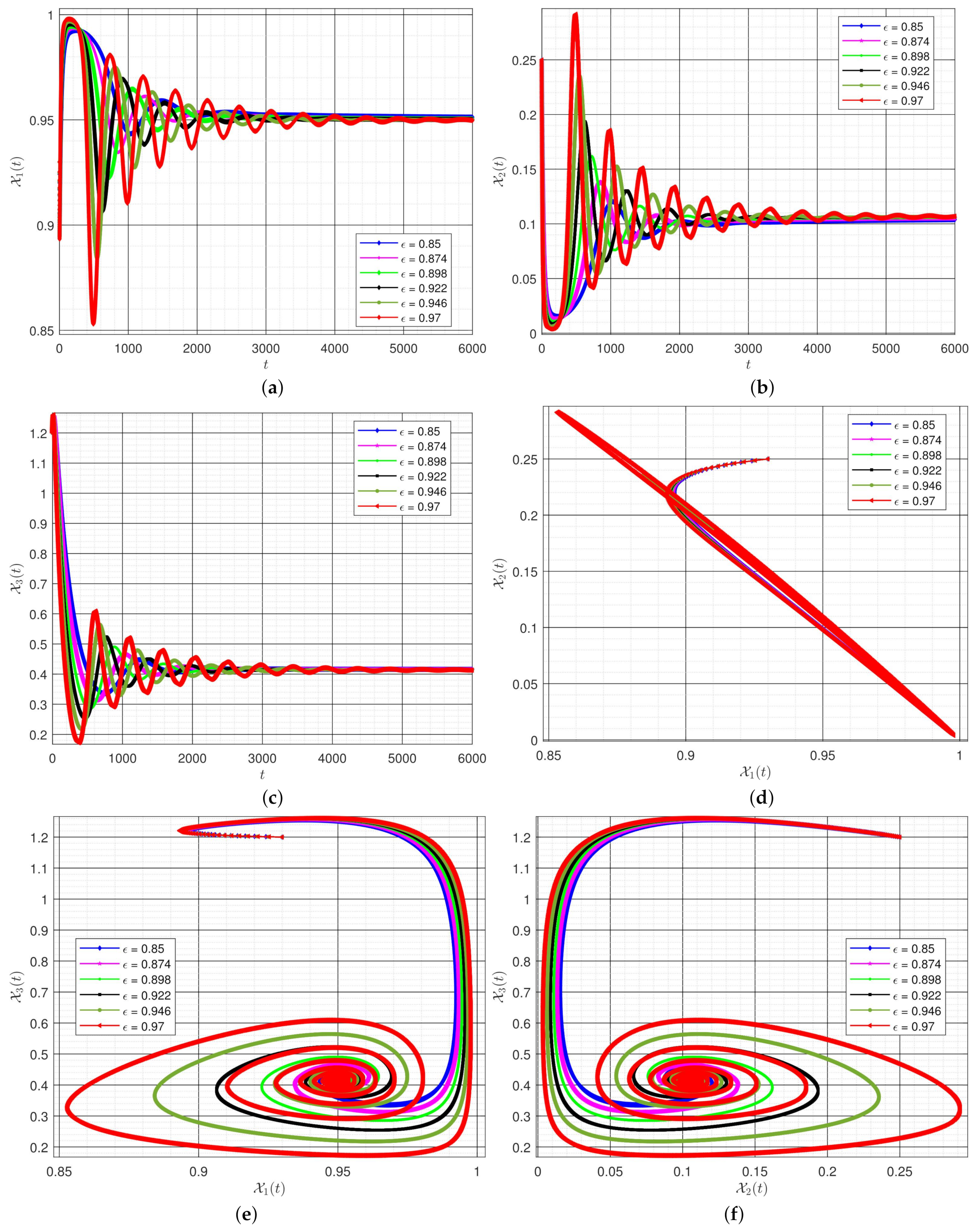
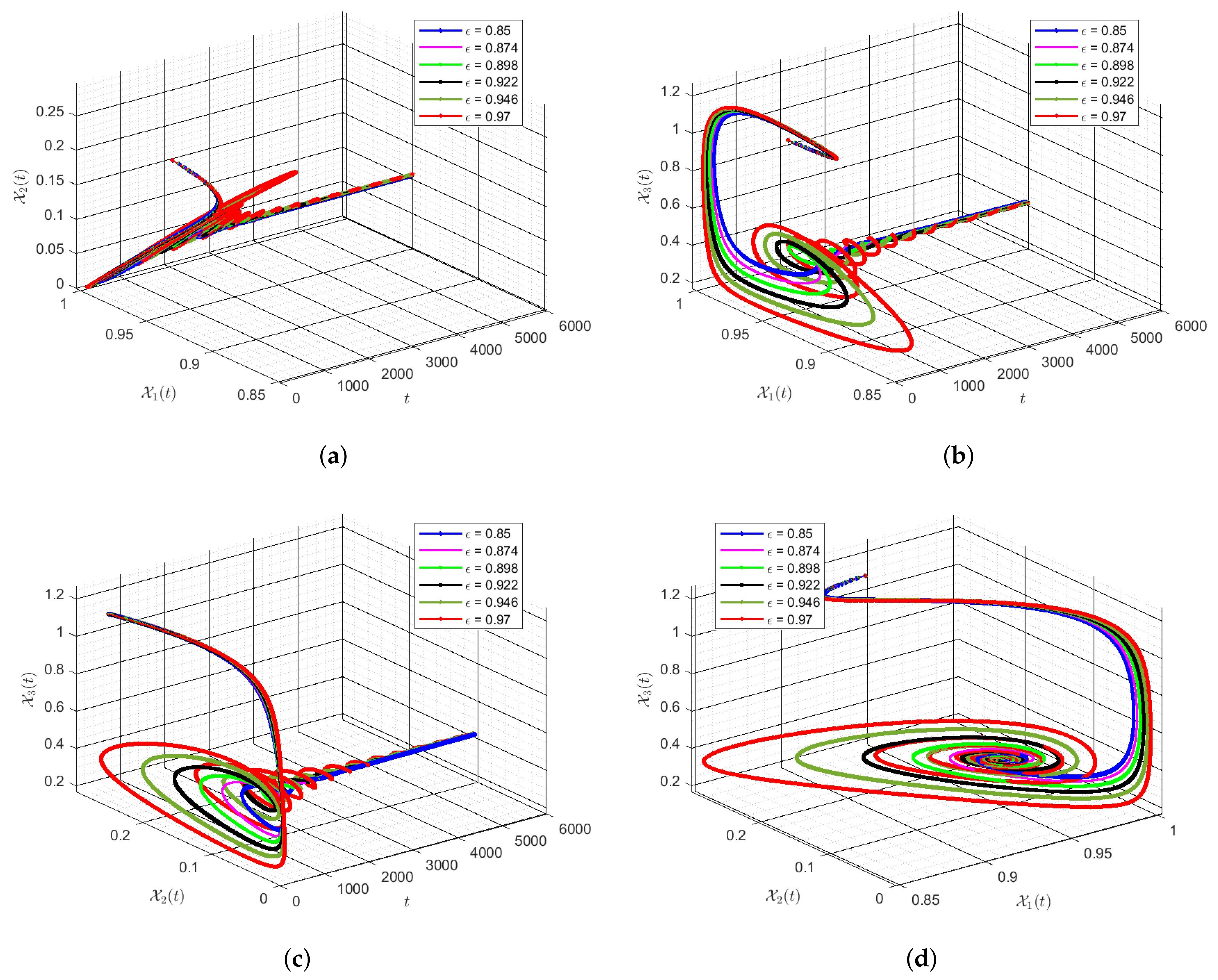
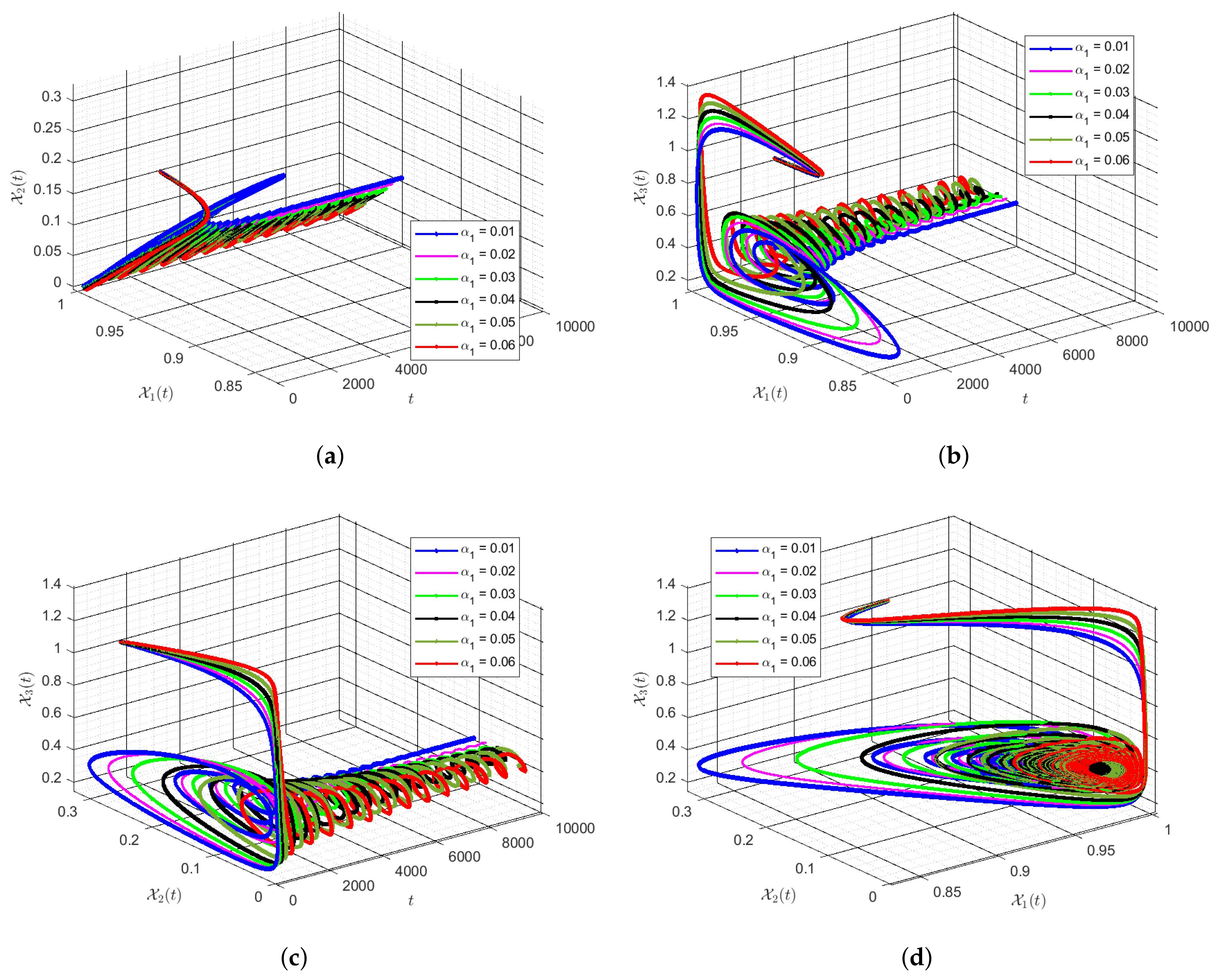
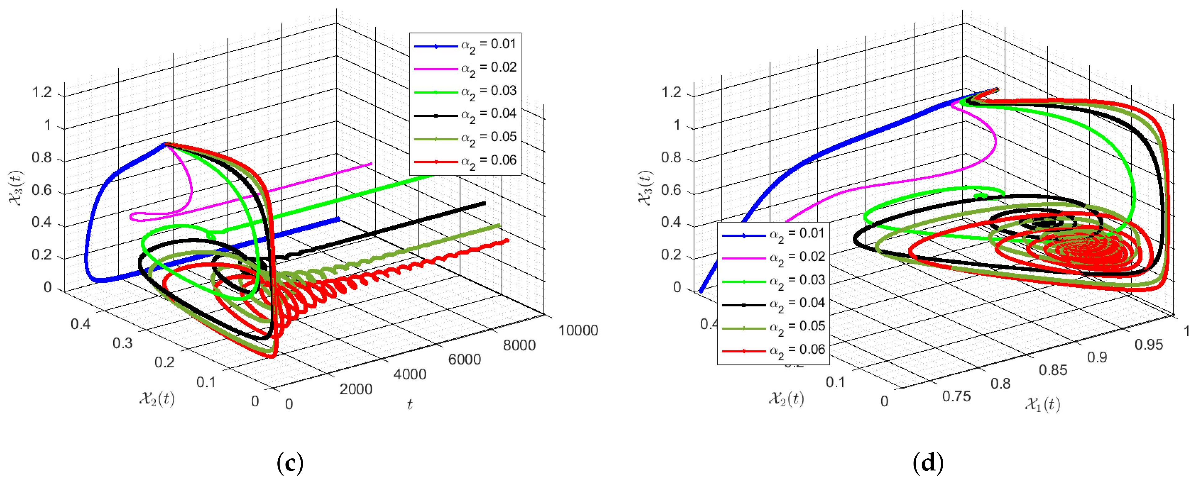
Now, we investigate the sensitivity of the model with respect to some of the parameters in the formulation presented in the system (14). First, we consider the values defined in (34) with $ϵ=0.95$ and examine the effect of $\beta$ on results via taking $0.57,0.58,0.59,0.6,0.61$, and $0.62$. Approximate solutions corresponding to these assumptions are shown in Figure 3 and Figure 4. In these plots, it is clear that as the amount of $\beta$ increased, the system tends to exhibit more malicious behavior. However, for smaller values, the system is stable and tends towards a certain equilibrium point.

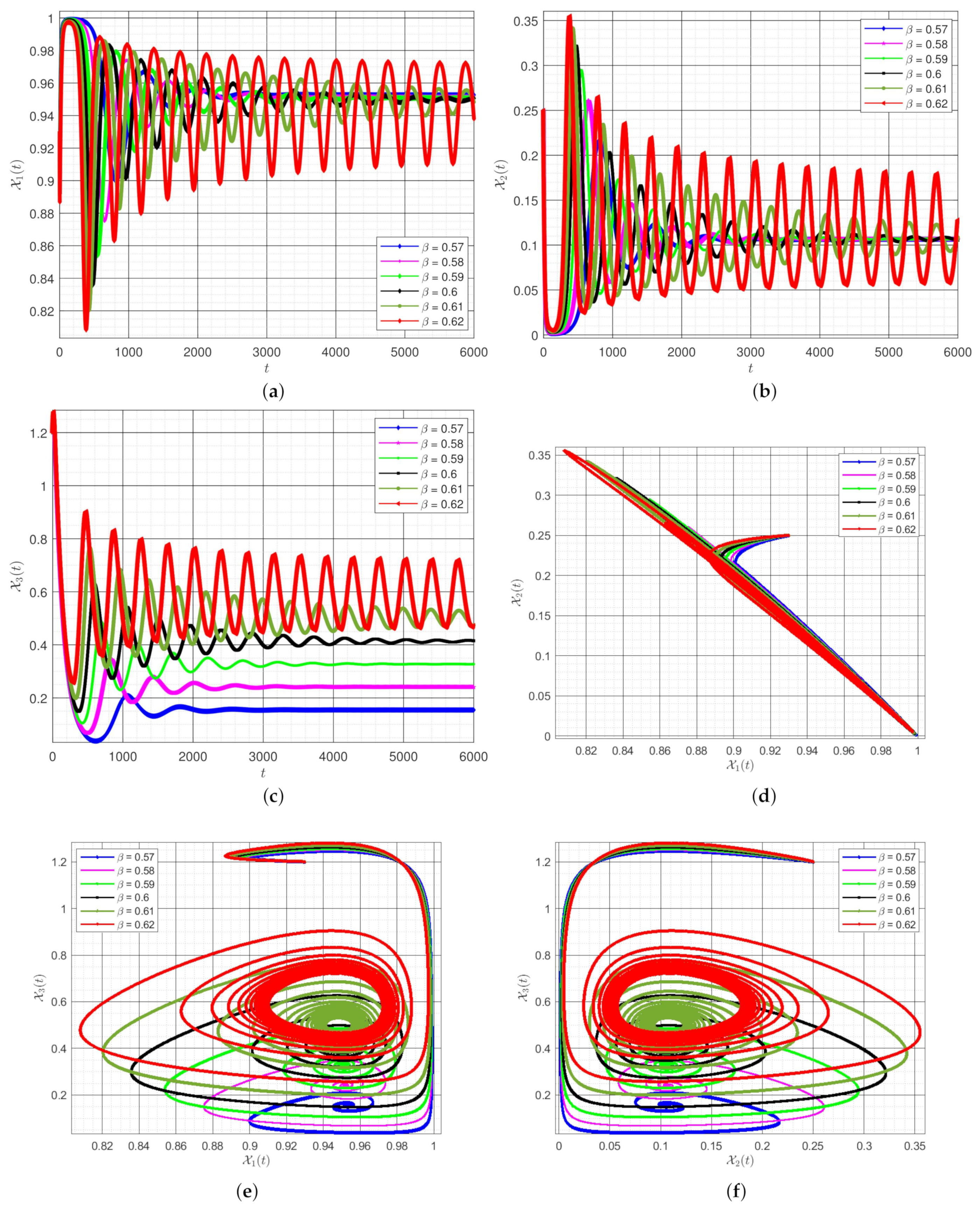
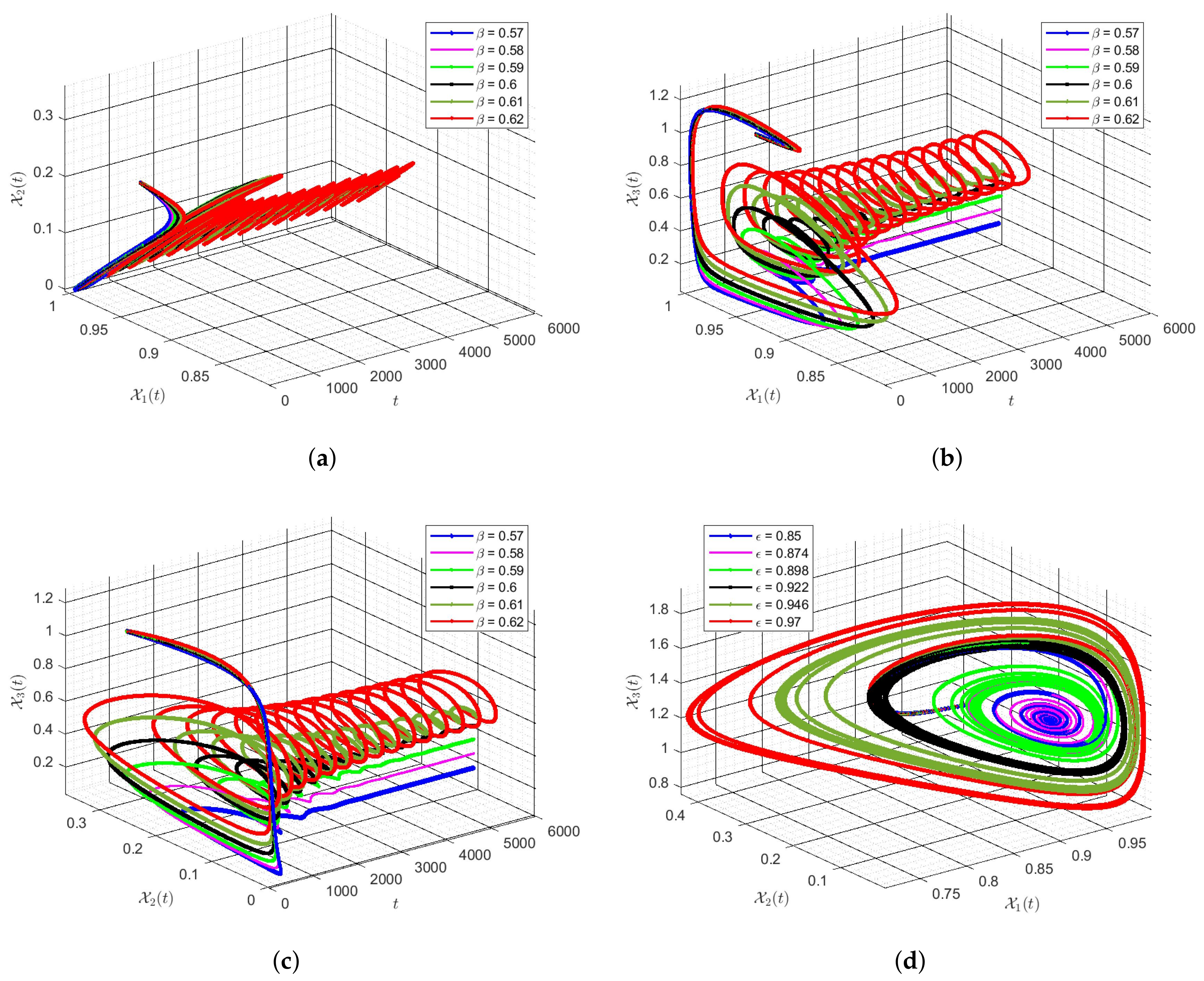
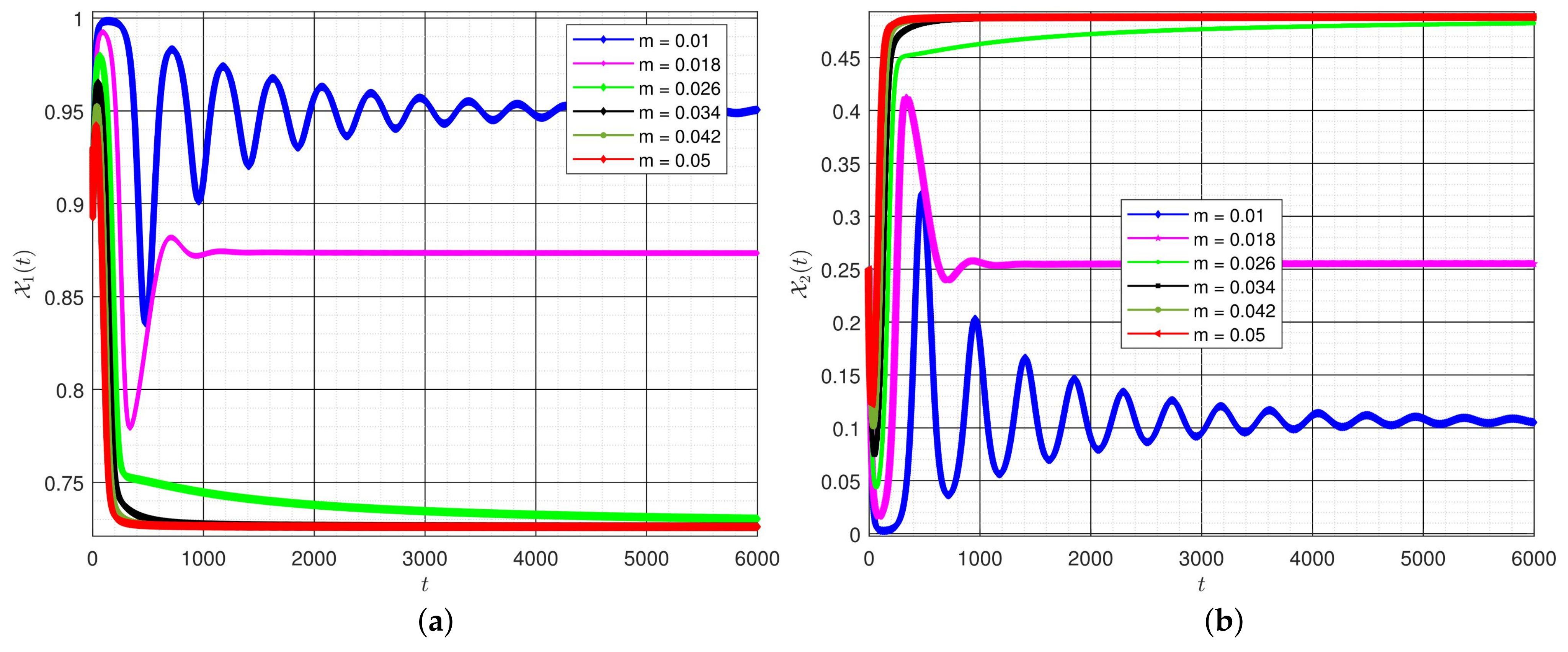
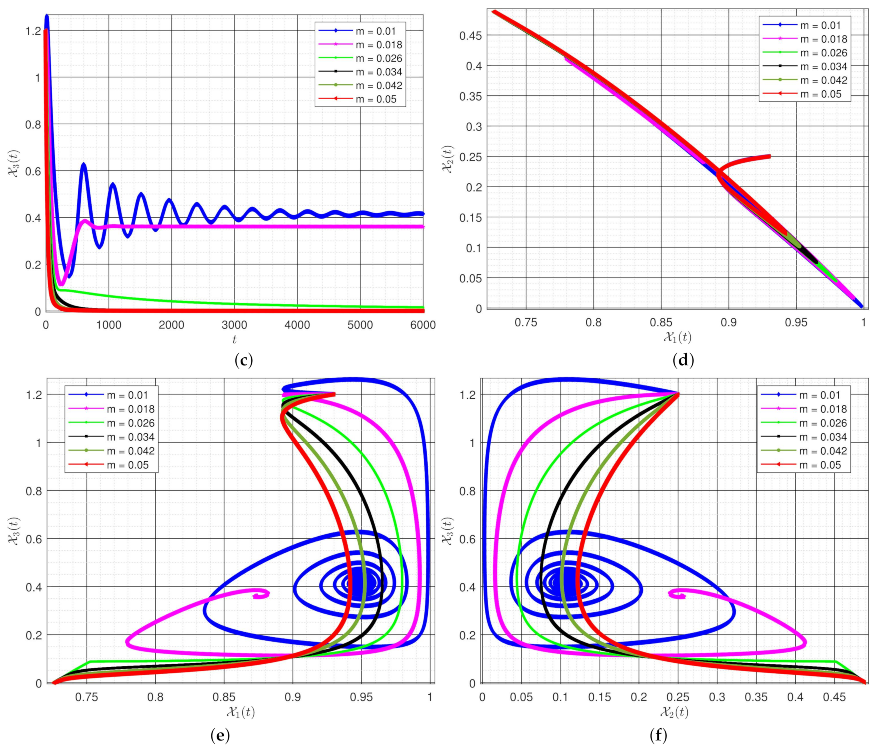
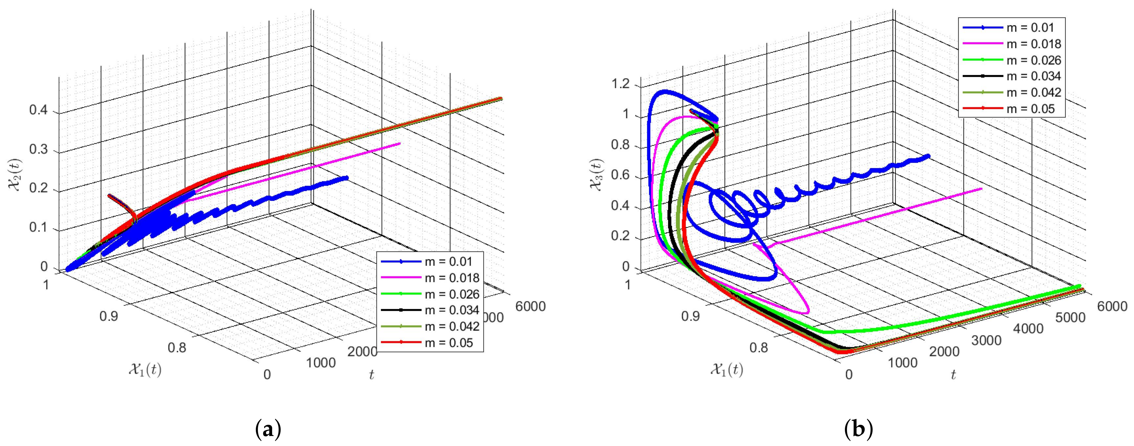
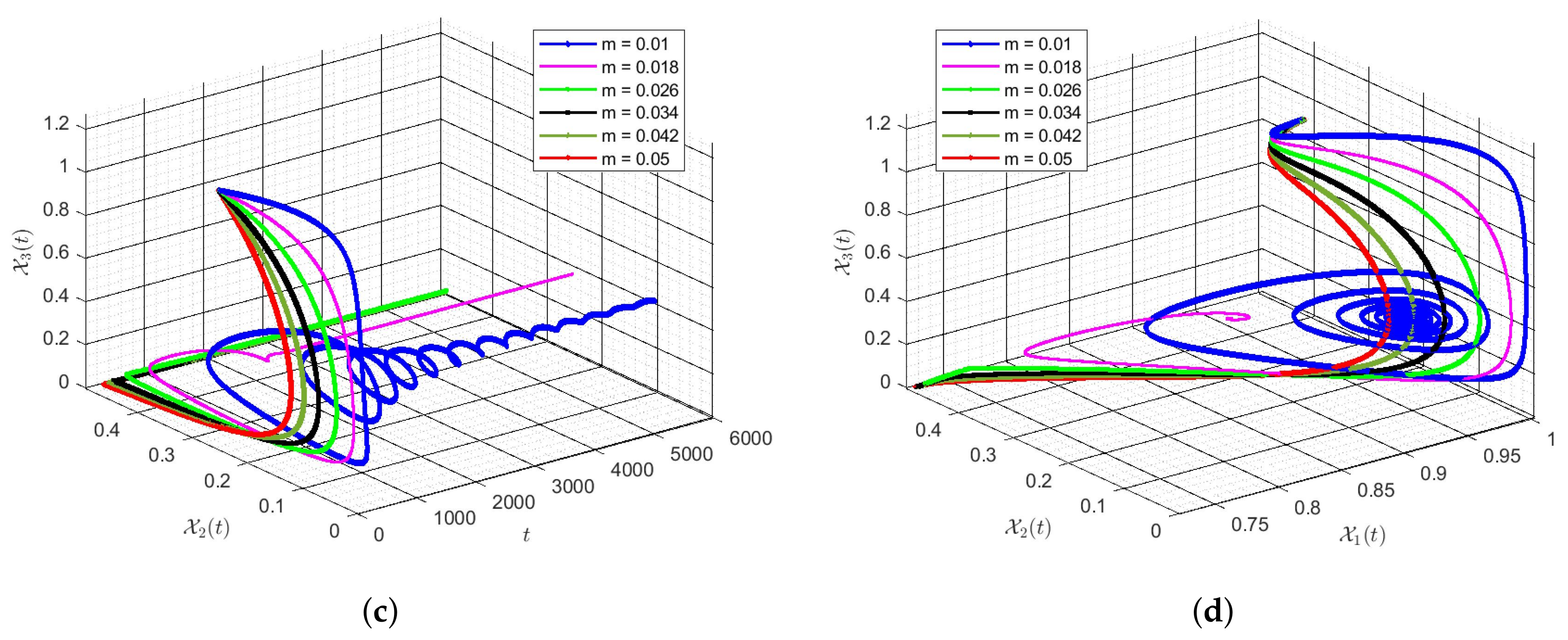
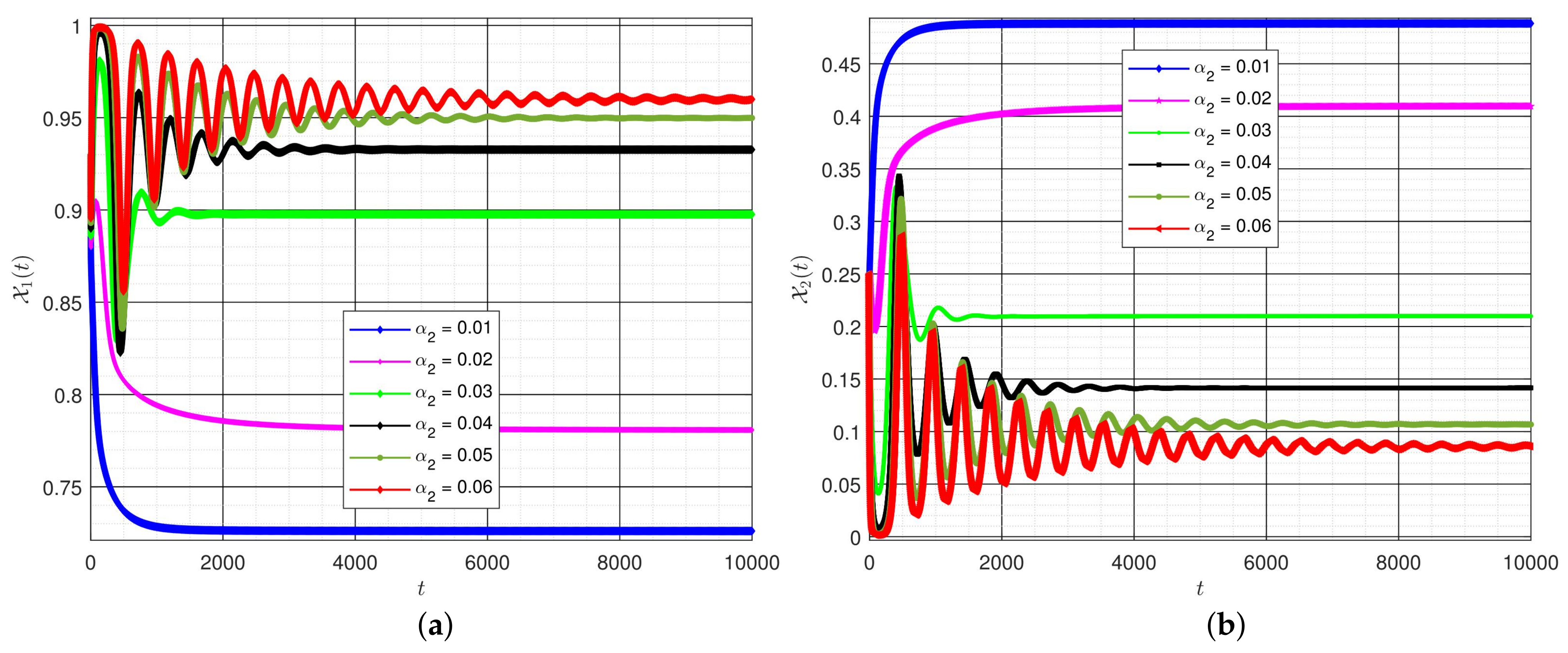
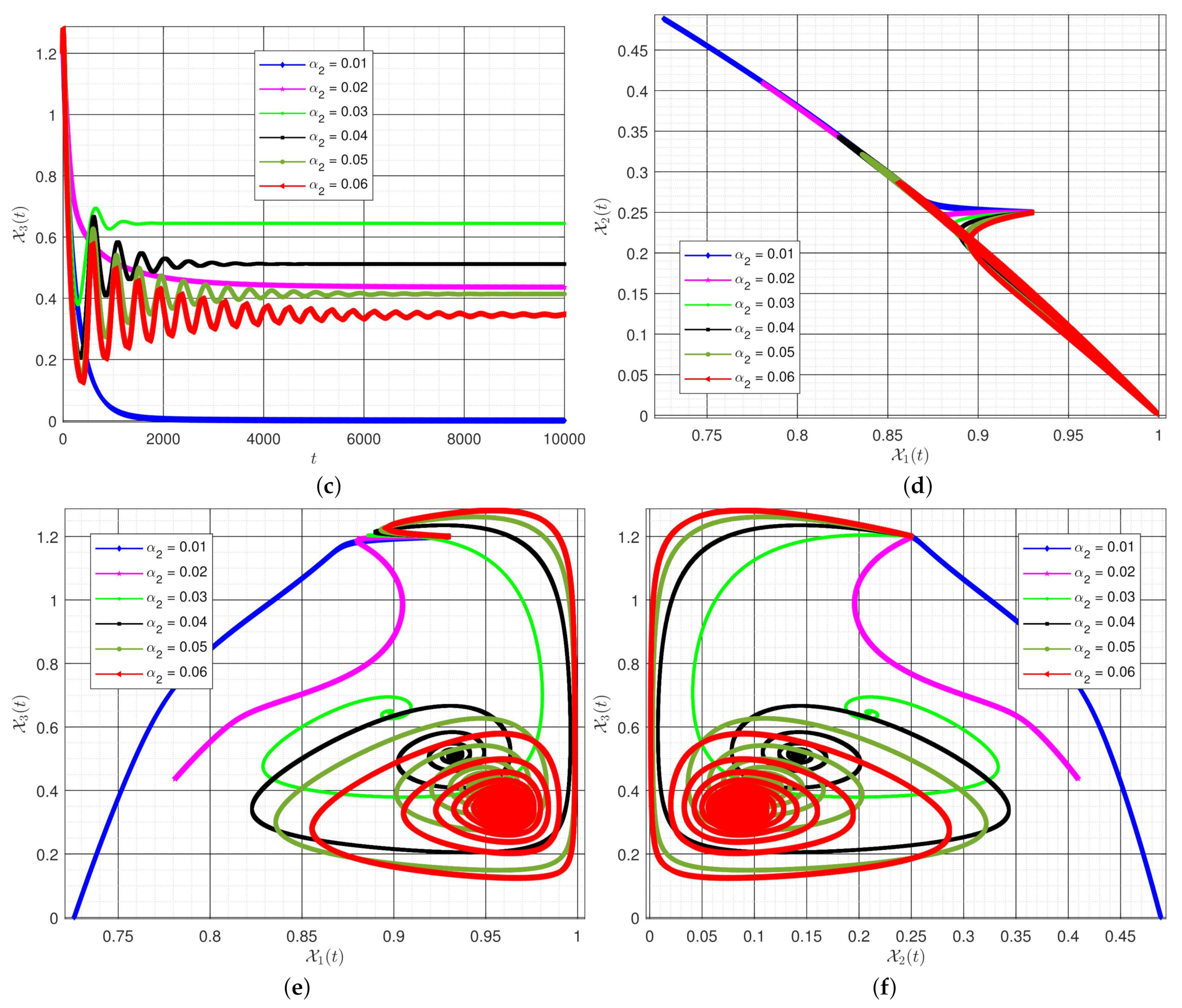
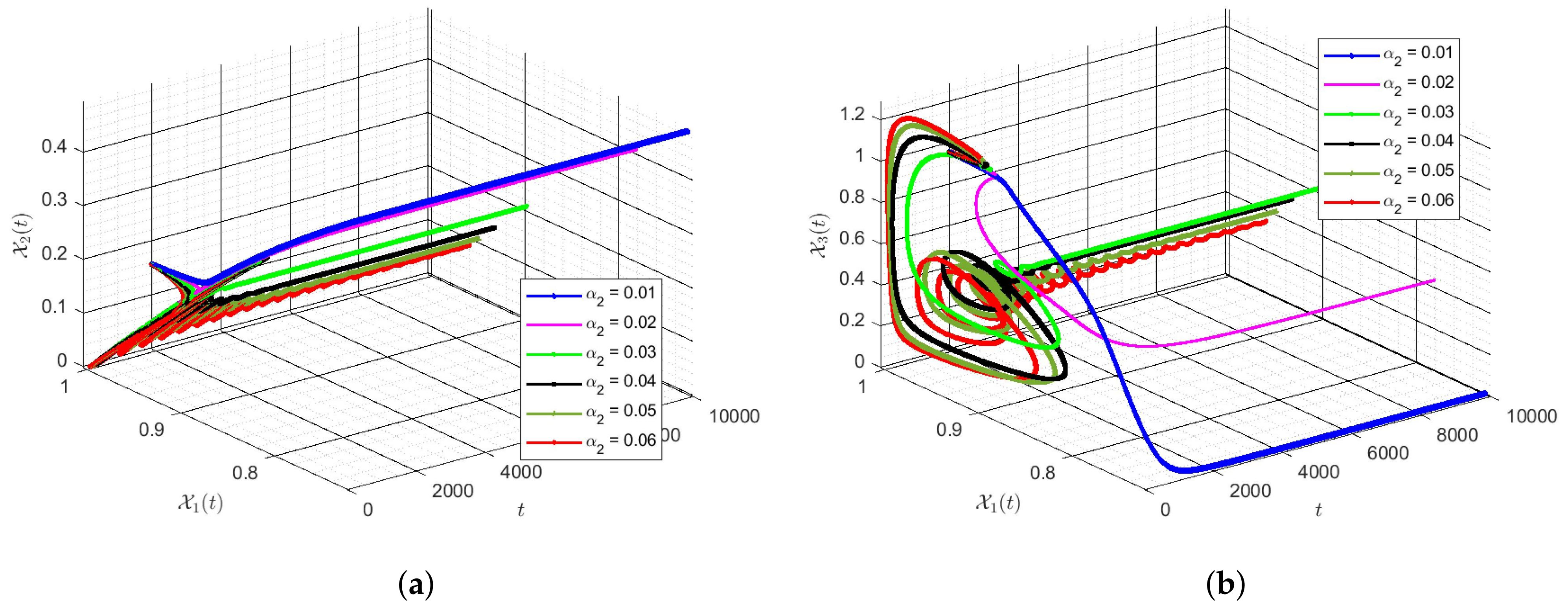
In this section, we look at the effect of parameter $m_1$ on model results. To this end, the values of $m_1$ are taken as $0.01,0.018,0.026,0.034,0.042$, and $0.05$. In Figure 5 and Figure 6, we have depicted the acquired approximate results by taking these values. The results show that a change in this value for the parameter will change the type of system equilibrium point.

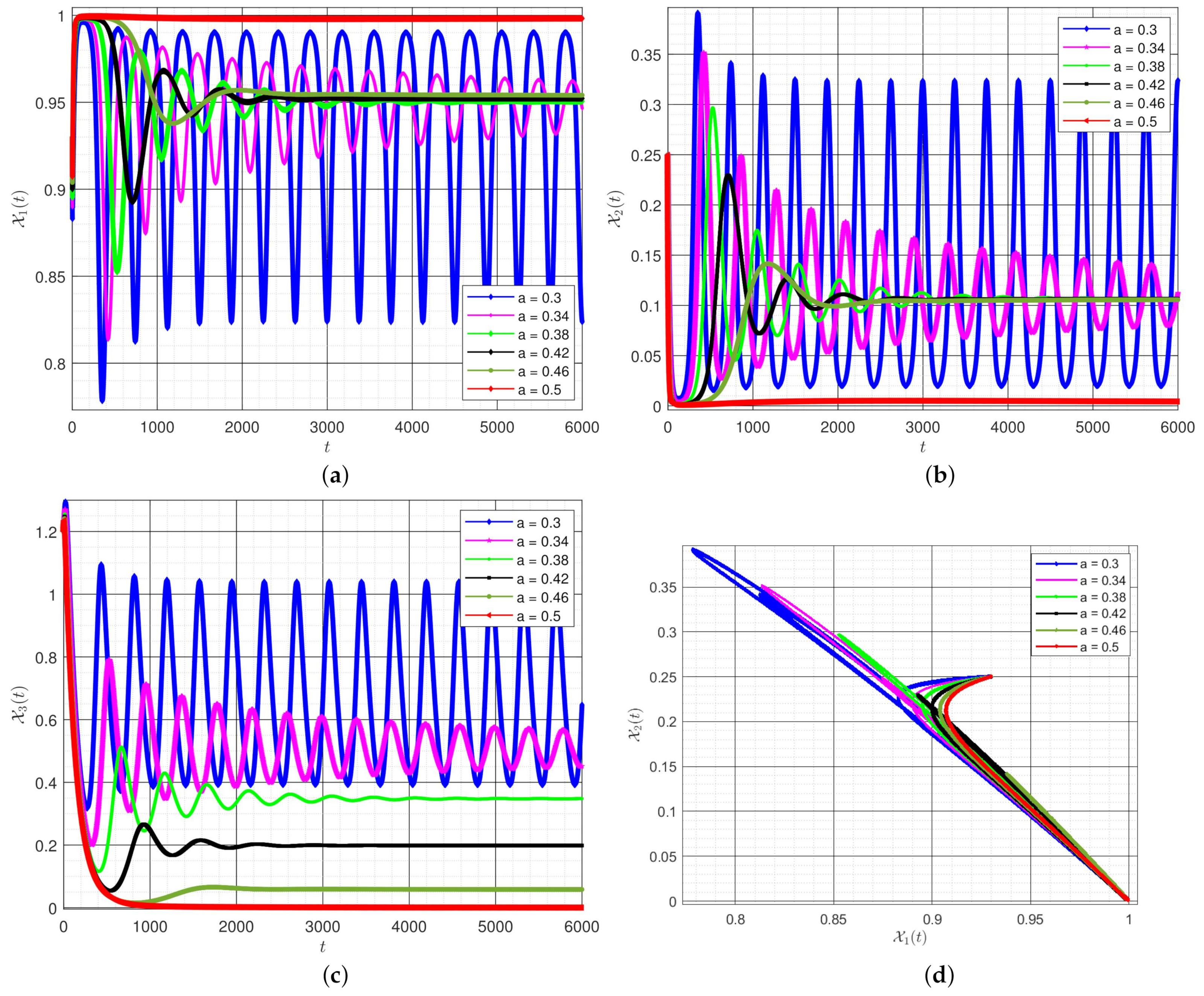
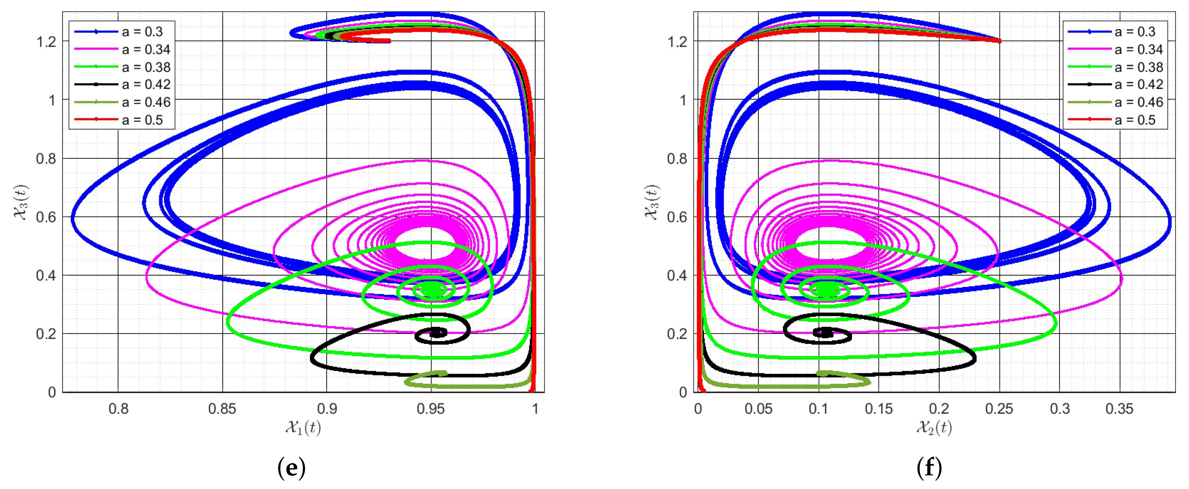
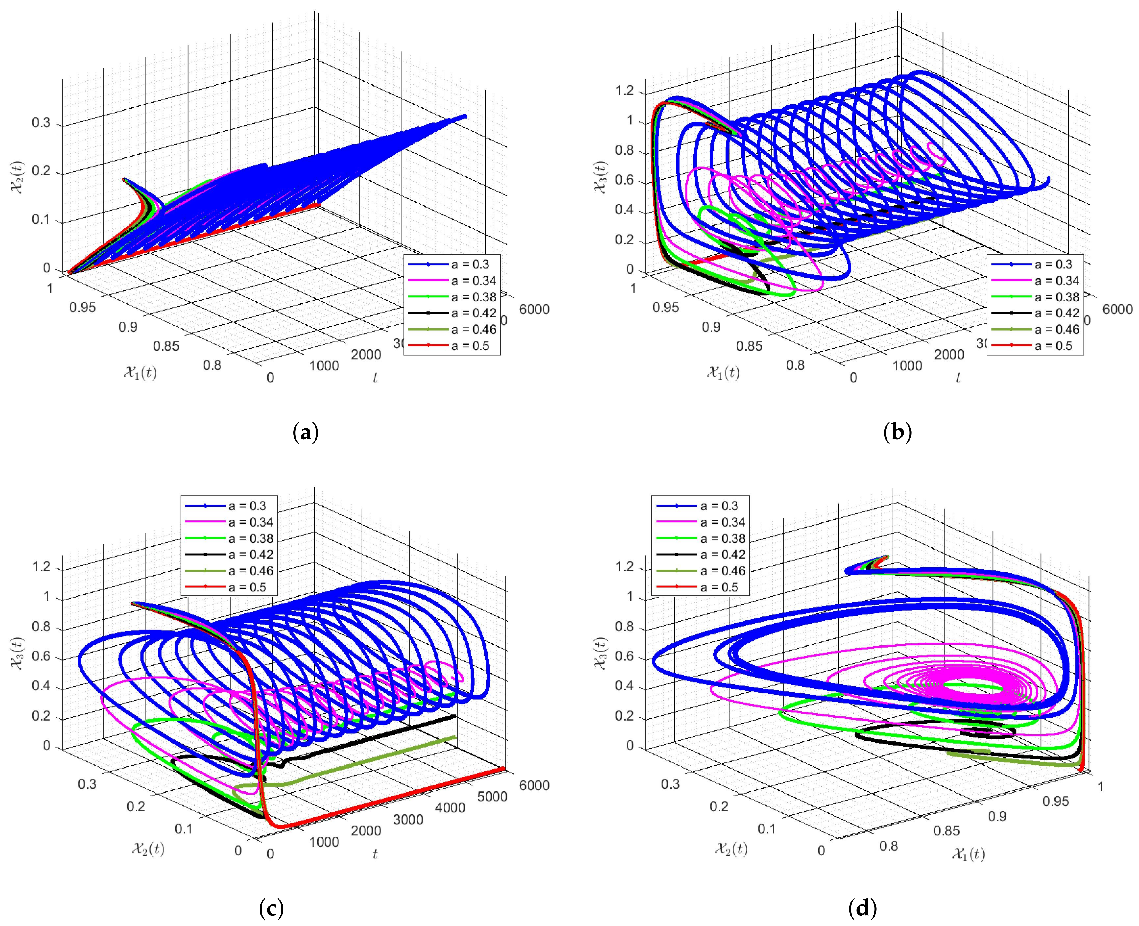
Moreover, we have examined the role of a through taking $0.3,0.34,$$0.38,0.42,0.46$, and $0.5$. Figure 7 and Figure 8 display corresponding to the obtained solutions of the system (14). Behaviors related to smaller values of a’s are more stable whilst for larger values of the parameter; a very severe oscillation behavior is evident in the system.

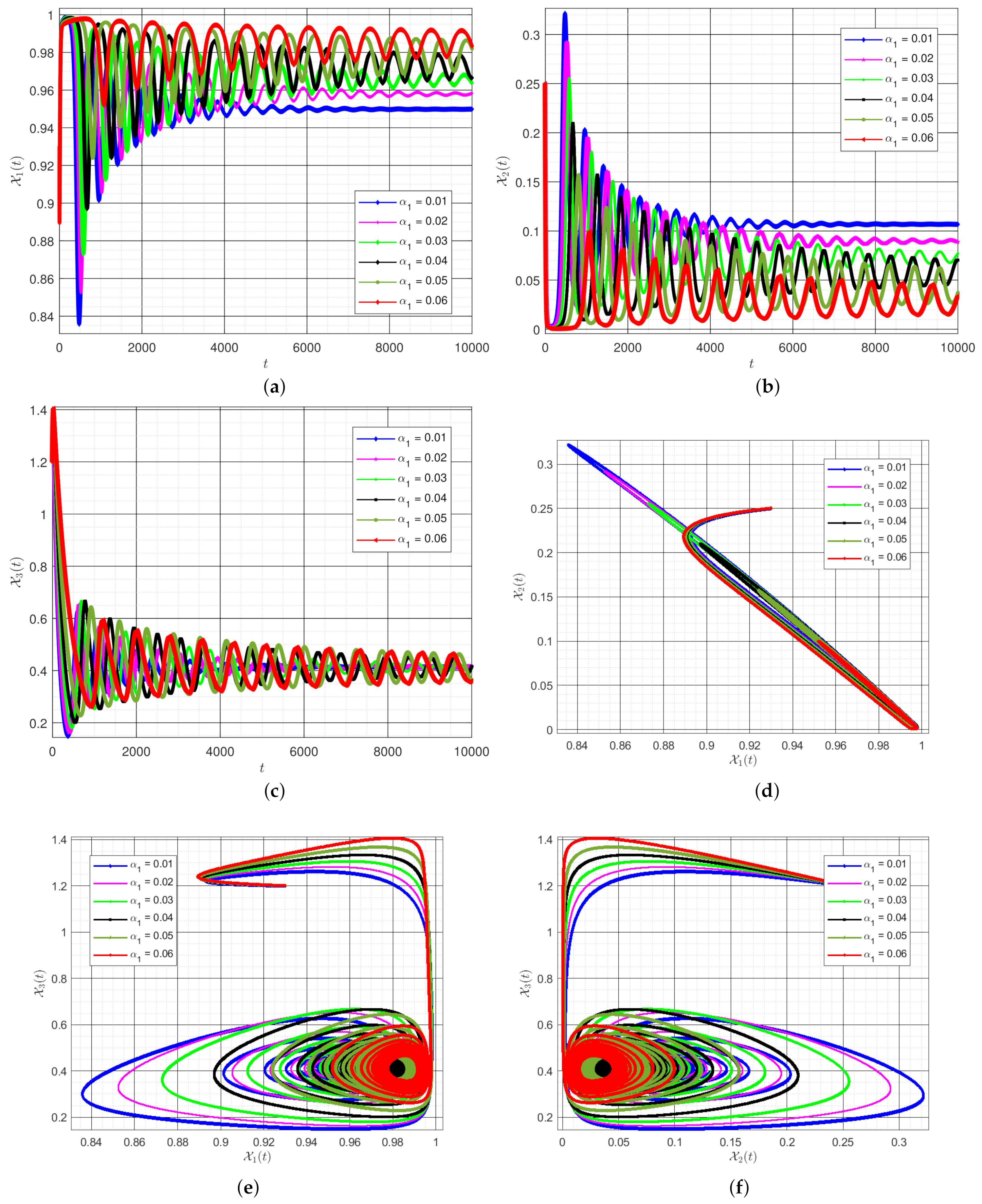
Then, we have taken the role of ${\alpha }_1$ on results via taking $0.01,0.02,0.03,0.04,0.05$, and $0.06$ in Figure 9 and Figure 10. In these graphs, it is clear that by increasing the value for ${\alpha }_1$, the behavior will be very chaotic and unstable.

Finally, we study the role of ${\alpha }_2$ on results through taking values $0.01,0.02,0.03,0.04,0.05$, and $0.06$ in Figure 11 and Figure 12.

The results obtained in these plots confirm that the system solution for each case converges to its different corresponding equilibrium points.

7. Conclusions

Eco-epidemiology can be considered as a meaningful combination of two research fields of ecology and epidemiology. These problems mainly take ecological systems into account epidemiological factors. By utilizing new modern mathematical tools, significant progress can be made in the modeling eco-epidemiological scenarios. By fully incorporating these elements, eco-epidemiology would be rooted in the investigation of the pathways by which biological and social experiences generate health and disease. In this contribution, the $\mathsf{AB}$ fractional derivative is employed to study some computational aspects of three species of the prey–predator model in mathematical biology. The concept of memory and symmetry are the main reasons for using these useful tools. According to the results obtained in this study, which is very compatible with the expected conditions, the method used in the article can be used to solve other problems in epidemiology. This can be considered as a direction for future research in describing other eco-epidemiological problems.

References

- Murray, J.D. Mathematical Biology: I. An Introduction; Springer Science & Business Media: Berlin/Heidelberg, Germany, 2007; Volume 17. [Google Scholar]
- De Vries, G.; Hillen, T.; Lewis, M.; Müller, J.; Schönfisch, B. A Course in Mathematical Biology: Quantitative Modeling with Mathematical and Computational Methods; SIAM: Philadelphia, PA, USA, 2006. [Google Scholar]
- Nabti, A.; Ghanbari, B. Global stability analysis of a fractional SVEIR epidemic model. Math. Methods Appl. Sci. 2021, 44, 8577–8597. [Google Scholar] [CrossRef]
- Anderson, R.M.; May, R.M. The population dynamics of microparasites and their invertebrate hosts. Philos. Trans. R. Soc. Lond. B Biol. Sci. 1981, 291, 451–524. [Google Scholar]
- Berezovskaya, F.S.; Song, B.; Castillo-Chavez, C. Role of prey dispersal and refuges on predator-prey dynamics. SIAM J. Appl. Math. 2010, 70, 1821–1839. [Google Scholar] [CrossRef]
- Djilali, S.; Ghanbari, B. Dynamical behavior of two predators–one prey model with generalized functional response and time-fractional derivative. Adv. Differ. Equ. 2021, 2021, 1–19. [Google Scholar] [CrossRef]
- Vineis, P. Exposomics: Mathematics meets biology. Mutagenesis 2015, 30, 719–722. [Google Scholar] [CrossRef] [Green Version]
- Bellomo, N.; Elaiw, A.; Althiabi, A.M.; Alghamdi, M.A. On the interplay between mathematics and biology: Hallmarks toward a new systems biology. Phys. Life Rev. 2015, 12, 44–64. [Google Scholar] [CrossRef]
- Djilali, S.; Bentout, S.; Ghanbari, B.; Kumar, S. Spatial patterns in a vegetation model with internal competition and feedback regulation. Eur. Phys. J. Plus 2021, 136, 1–24. [Google Scholar] [CrossRef]
- Levin, S.A. Frontiers in Mathematical Biology; Springer: Berlin, Germany, 1994. [Google Scholar]
- Britton, N. Essential Mathematical Biology; Springer Science & Business Media: Berlin/Heidelberg, Germany, 2005. [Google Scholar]
- Ghanbari, B.; Gómez-Aguilar, J. Analysis of two avian influenza epidemic models involving fractal-fractional derivatives with power and Mittag-Leffler memories. Chaos Interdiscip. J. Nonlinear Sci. 2019, 29, 123113. [Google Scholar] [CrossRef] [PubMed]
- Ghanbari, B.; Günerhan, H.; Srivastava, H. An application of the Atangana-Baleanu fractional derivative in mathematical biology: A three-species predator-prey model. Chaos Solitons Fractals 2020, 138, 109910. [Google Scholar] [CrossRef]
- Jena, R.M.; Chakraverty, S.; Rezazadeh, H.; Domiri Ganji, D. On the solution of time-fractional dynamical model of Brusselator reaction-diffusion system arising in chemical reactions. Math. Methods Appl. Sci. 2020, 43, 3903–3913. [Google Scholar] [CrossRef]
- Ghanbari, B. On novel nondifferentiable exact solutions to local fractional Gardner’s equation using an effective technique. Math. Methods Appl. Sci. 2021, 44, 4673–4685. [Google Scholar] [CrossRef]
- Aminikhah, H.; Sheikhani, A.H.R.; Houlari, T.; Rezazadeh, H. Numerical solution of the distributed-order fractional Bagley-Torvik equation. IEEE/CAA J. Autom. Sin. 2017, 6, 760–765. [Google Scholar] [CrossRef]
- Ghanbari, B.; Yusuf, A.; Baleanu, D. The new exact solitary wave solutions and stability analysis for the (2 + 1) (2+1)-dimensional Zakharov–Kuznetsov equation. Adv. Differ. Equ. 2019, 2019, 49. [Google Scholar] [CrossRef] [Green Version]
- Rahman, G.; Nisar, K.S.; Ghanbari, B.; Abdeljawad, T. On generalized fractional integral inequalities for the monotone weighted Chebyshev functionals. Adv. Differ. Equ. 2020, 2020, 368. [Google Scholar] [CrossRef]
- Srinivasa, K.; Rezazadeh, H. Numerical solution for the fractional-order one-dimensional telegraph equation via wavelet technique. Int. J. Nonlinear Sci. Numer. Simul. 2020, 1. [Google Scholar] [CrossRef]
- Ghanbari, B.; Nisar, K.S.; Aldhaifallah, M. Abundant solitary wave solutions to an extended nonlinear Schrödinger’s equation with conformable derivative using an efficient integration method. Adv. Differ. Equ. 2020, 2020, 328. [Google Scholar] [CrossRef]
- Ahmed, N.; Rafiq, M.; Adel, W.; Rezazadeh, H.; Khan, I.; Nisar, K.S. Structure Preserving Numerical Analysis of HIV and CD4+ T-Cells Reaction Diffusion Model in Two Space Dimensions. Chaos Solitons Fractals 2020, 139, 110307. [Google Scholar] [CrossRef]
- Jones, D.S.; Plank, M.; Sleeman, B.D. Differential Equations and Mathematical Biology; CRC Press: Boca Raton, FL, USA, 2009. [Google Scholar]
- Ghanbari, B.; Kumar, S. A study on fractional predator–prey–pathogen model with Mittag–Leffler kernel-based operators. Numer. Methods Partial. Differ. Equ. 2020. [Google Scholar] [CrossRef]
- Inan, B.; Osman, M.S.; Ak, T.; Baleanu, D. Analytical and numerical solutions of mathematical biology models: The Newell-Whitehead-Segel and Allen-Cahn equations. Math. Methods Appl. Sci. 2020, 43, 2588–2600. [Google Scholar] [CrossRef]
- Ghanbari, B. Abundant exact solutions to a generalized nonlinear Schrödinger equation with local fractional derivative. Math. Methods Appl. Sci. 2021, 44, 8759–8774. [Google Scholar] [CrossRef]
- Ghanbari, B.; Rada, L. Solitary wave solutions to the Tzitzeica type equations obtained by a new efficient approach. J. Appl. Anal. Comput. 2019, 9, 568–589. [Google Scholar] [CrossRef]
- Srivastava, H.M.; Günerhan, H.; Ghanbari, B. Exact traveling wave solutions for resonance nonlinear Schrödinger equation with intermodal dispersions and the Kerr law nonlinearity. Math. Methods Appl. Sci. 2019, 42, 7210–7221. [Google Scholar] [CrossRef]
- Ghanbari, B.; Djilali, S. Mathematical analysis of a fractional-order predator-prey model with prey social behavior and infection developed in predator population. Chaos Solitons Fractals 2020, 138, 109960. [Google Scholar] [CrossRef]
- Munusamy, K.; Ravichandran, C.; Nisar, K.S.; Ghanbari, B. Existence of solutions for some functional integrodifferential equations with nonlocal conditions. Math. Methods Appl. Sci. 2020, 43, 10319–10331. [Google Scholar] [CrossRef]
- Ahmad, I.; Ahmad, H.; Thounthong, P.; Chu, Y.M.; Cesarano, C. Solution of multi-term time-fractional PDE models arising in mathematical biology and physics by local meshless method. Symmetry 2020, 12, 1195. [Google Scholar] [CrossRef]
- Khan, Y.; Vazquez-Leal, H.; Wu, Q. An efficient iterated method for mathematical biology model. Neural Comput. Appl. 2013, 23, 677–682. [Google Scholar] [CrossRef]
- Kaur, D.; Agarwal, P.; Rakshit, M.; Chand, M. Fractional Calculus involving (p, q)-Mathieu Type Series. Appl. Math. Nonlinear Sci. 2020, 5, 15–34. [Google Scholar] [CrossRef]
- Gençoglu, M.T.; Agarwal, P. Use of Quantum Differential Equations in Sonic Processes. Appl. Math. Nonlinear Sci. 2020, 6, 21–28. [Google Scholar] [CrossRef]
- Aidara, S.; Sagna, Y. BSDEs driven by two mutually independent fractional Brownian motions with stochastic Lipschitz coefficients. Appl. Math. Nonlinear Sci. 2019, 4, 139–150. [Google Scholar] [CrossRef] [Green Version]
- Wu, J.; Yuan, J.; Gao, W. Analysis of fractional factor system for data transmission in SDN. Appl. Math. Nonlinear Sci. 2019, 4, 191–196. [Google Scholar] [CrossRef] [Green Version]
- Al-Ghafri, K.S.; Rezazadeh, H. Solitons and other solutions of (3 + 1)-dimensional space–time fractional modified KdV–Zakharov–Kuznetsov equation. Appl. Math. Nonlinear Sci. 2019, 4, 289–304. [Google Scholar] [CrossRef] [Green Version]
- Ziane, D.; Cherif, M.H.; Cattani, C.; Belghaba, K. Yang-Laplace Decomposition Method for Nonlinear System of Local Fractional Partial Differential Equations. Appl. Math. Nonlinear Sci. 2019, 4, 489–502. [Google Scholar] [CrossRef] [Green Version]
- Sulaiman, T.A.; Bulut, H.; Atas, S.S. Optical solitons to the fractional Schrdinger-Hirota equation. Appl. Math. Nonlinear Sci. 2019, 4, 535–542. [Google Scholar] [CrossRef] [Green Version]
- İlhan, E.; Kıymaz, İ.O. A generalization of truncated M-fractional derivative and applications to fractional differential equations. Appl. Math. Nonlinear Sci. 2020, 5, 171–188. [Google Scholar]
- Biswas, S.; Sasmal, S.K.; Samanta, S.; Saifuddin, M.; Pal, N.; Chattopadhyay, J. Optimal harvesting and complex dynamics in a delayed eco-epidemiological model with weak Allee effects. Nonlinear Dyn. 2017, 87, 1553–1573. [Google Scholar] [CrossRef]
- Saifuddin, M.; Samanta, S.; Biswas, S.; Chattopadhyay, J. An eco-epidemiological model with different competition coefficients and strong-Allee in the prey. Int. J. Bifurc. Chaos 2017, 27, 1730027. [Google Scholar] [CrossRef]
- Saifuddin, M.; Biswas, S.; Samanta, S.; Sarkar, S.; Chattopadhyay, J. Complex dynamics of an eco-epidemiological model with different competition coefficients and weak Allee in the predator. Chaos Solitons Fractals 2016, 91, 270–285. [Google Scholar] [CrossRef]
- Naik, P.A.; Zu, J.; Ghoreishi, M. Stability analysis and approximate solution of SIR epidemic model with crowley-martin type functional response and Holling type-II treatment rate by using homotopy analysis method. J. Appl. Anal. Comput. 2020, 10, 1482–1515. [Google Scholar]
- Yavuz, M.; Özdemir, N. Comparing the new fractional derivative operators involving exponential and Mittag-Leffler kernel. Discret. Contin. Dyn. Syst. S 2020, 13, 995. [Google Scholar] [CrossRef] [Green Version]
- Naik, P.A.; Zu, J.; Owolabi, K.M. Modeling the mechanics of viral kinetics under immune control during primary infection of HIV-1 with treatment in fractional order. Phys. A Stat. Mech. Its Appl. 2020, 545, 123816. [Google Scholar] [CrossRef]
- Yavuz, M.; Yokus, A. Analytical and numerical approaches to nerve impulse model of fractional-order. Numer. Methods Partial. Differ. Equ. 2020, 36, 1348–1368. [Google Scholar] [CrossRef]
- Owolabi, K.M.; Gómez-Aguilar, J.; Karaagac, B. Modelling, analysis and simulations of some chaotic systems using derivative with Mittag–Leffler kernel. Chaos Solitons Fractals 2019, 125, 54–63. [Google Scholar] [CrossRef]
- Qureshi, S.; Atangana, A. Fractal-fractional differentiation for the modeling and mathematical analysis of nonlinear diarrhea transmission dynamics under the use of real data. Chaos Solitons Fractals 2020, 136, 109812. [Google Scholar] [CrossRef]
- Ul Rehman, A.; Singh, R.; Agarwal, P. Modeling, analysis and prediction of new variants of covid-19 and dengue co-infection on complex network. Chaos Solitons Fractals 2021, 150, 111008. [Google Scholar] [CrossRef] [PubMed]
- Agarwal, P.; Singh, R. Modelling of transmission dynamics of Nipah virus (Niv): A fractional order approach. Phys. A Stat. Mech. Its Appl. 2020, 547, 124243. [Google Scholar] [CrossRef]
- Ghanbari, B.; Atangana, A. A new application of fractional Atangana–Baleanu derivatives: Designing ABC-fractional masks in image processing. Phys. A Stat. Mech. Its Appl. 2020, 542, 123516. [Google Scholar] [CrossRef]
- Lizzy, R.M.; Balachandran, K.; Trujillo, J.J. Controllability of nonlinear stochastic fractional neutral systems with multiple time varying delays in control. Chaos Solitons Fractals 2017, 102, 162–167. [Google Scholar] [CrossRef]
- Jajarmi, A.; Yusuf, A.; Baleanu, D.; Inc, M. A new fractional HRSV model and its optimal control: A non-singular operator approach. Phys. A Stat. Mech. Its Appl. 2020, 547, 123860. [Google Scholar] [CrossRef]
- Ghanbari, B.; Atangana, A. Some new edge detecting techniques based on fractional derivatives with non-local and non-singular kernels. Adv. Differ. Equ. 2020, 2020, 435. [Google Scholar] [CrossRef]
- Mazzoleni, S.; Russo, L.; Giannino, F.; Toraldo, G.; Siettos, C. Mathematical modelling and numerical bifurcation analysis of inbreeding and interdisciplinarity dynamics in academia. J. Comput. Appl. Math. 2021, 385, 113194. [Google Scholar] [CrossRef]
- Djilali, S.; Ghanbari, B.; Bentout, S.; Mezouaghi, A. Turing-Hopf bifurcation in a diffusive mussel-algae model with time-fractional-order derivative. Chaos Solitons Fractals 2020, 138, 109954. [Google Scholar] [CrossRef]
- Babaei, A.; Ahmadi, M.; Jafari, H.; Liya, A. A mathematical model to examine the effect of quarantine on the spread of coronavirus. Chaos Solitons Fractals 2021, 142, 110418. [Google Scholar] [CrossRef] [PubMed]
- Cressman, R.; Garay, J. A predator–prey refuge system: Evolutionary stability in ecological systems. Theor. Popul. Biol. 2009, 76, 248–257. [Google Scholar] [CrossRef] [PubMed]
- Chen, S.; Wei, J.; Yu, J. Stationary patterns of a diffusive predator–prey model with Crowley–Martin functional response. Nonlinear Anal. Real World Appl. 2018, 39, 33–57. [Google Scholar] [CrossRef] [Green Version]
- Ghanbari, B.; Djilali, S. Mathematical and numerical analysis of a three-species predator-prey model with herd behavior and time fractional-order derivative. Math. Methods Appl. Sci. 2020, 43, 1736–1752. [Google Scholar] [CrossRef]
- Agarwal, P.; Singh, R.; ul Rehman, A. Numerical solution of hybrid mathematical model of dengue transmission with relapse and memory via Ada–Bashforth–Moulton predictor-corrector scheme. Chaos Solitons Fractals 2021, 143, 110564. [Google Scholar] [CrossRef]
- Owolabi, K.M. High-dimensional spatial patterns in fractional reaction-diffusion system arising in biology. Chaos Solitons Fractals 2020, 134, 109723. [Google Scholar] [CrossRef]
- Owolabi, K.M.; Atangana, A. Mathematical Modelling and Analysis of Fractional Epidemic Models Using Derivative with Exponential Kernel. In Fractional Calculus in Medical and Health Science; CRC Press: Boca Raton, FL, USA, 2020; pp. 109–128. [Google Scholar]
- Ghanbari, B. A new model for investigating the transmission of infectious diseases in a prey-predator system using a non-singular fractional derivative. Math. Methods Appl. Sci. 2021. [Google Scholar] [CrossRef]
- Allahviranloo, T.; Ghanbari, B. On the fuzzy fractional differential equation with interval Atangana–Baleanu fractional derivative approach. Chaos Solitons Fractals 2020, 130, 109397. [Google Scholar] [CrossRef]
- Wang, J.L.; Li, H.F. Memory-dependent derivative versus fractional derivative (I): Difference in temporal modeling. J. Comput. Appl. Math. 2021, 384, 112923. [Google Scholar] [CrossRef]
- Jajarmi, A.; Ghanbari, B.; Baleanu, D. A new and efficient numerical method for the fractional modeling and optimal control of diabetes and tuberculosis co-existence. Chaos Interdiscip. J. Nonlinear Sci. 2019, 29, 093111. [Google Scholar] [CrossRef]
- Abouelregal, A.E.; Moustapha, M.V.; Nofal, T.A.; Rashid, S.; Ahmad, H. Generalized thermoelasticity based on higher-order memory-dependent derivative with time delay. Res. Phys. 2021, 20, 103705. [Google Scholar]
- Ghanbari, B.; Gómez-Aguilar, J. Modeling the dynamics of nutrient–phytoplankton–zooplankton system with variable-order fractional derivatives. Chaos Solitons Fractals 2018, 116, 114–120. [Google Scholar] [CrossRef]
- Inc, M.; Acay, B.; Berhe, H.W.; Yusuf, A.; Khan, A.; Yao, S.W. Analysis of novel fractional COVID-19 model with real-life data application. Res. Phys. 2021, 23, 103968. [Google Scholar]
- Jahanshahi, H.; Munoz-Pacheco, J.M.; Bekiros, S.; Alotaibi, N.D. A fractional-order SIRD model with time-dependent memory indexes for encompassing the multi-fractional characteristics of the COVID-19. Chaos Solitons Fractals 2021, 143, 110632. [Google Scholar] [CrossRef]
- Ghanbari, B. On forecasting the spread of the COVID-19 in Iran: The second wave. Chaos Solitons Fractals 2020, 140, 110176. [Google Scholar] [CrossRef]
- Oud, M.A.A.; Ali, A.; Alrabaiah, H.; Ullah, S.; Khan, M.A.; Islam, S. A fractional order mathematical model for COVID-19 dynamics with quarantine, isolation, and environmental viral load. Adv. Differ. Equ. 2021, 2021, 106. [Google Scholar] [CrossRef] [PubMed]
- Furati, K.; Sarumi, I.; Khaliq, A. Fractional model for the spread of COVID-19 subject to government intervention and public perception. Appl. Math. Model. 2021, 95, 89–105. [Google Scholar] [CrossRef]
- Djilali, S.; Ghanbari, B. Coronavirus pandemic: A predictive analysis of the peak outbreak epidemic in South Africa, Turkey, and Brazil. Chaos Solitons Fractals 2020, 138, 109971. [Google Scholar] [CrossRef]
- Higazy, M. Novel fractional order SIDARTHE mathematical model of COVID-19 pandemic. Chaos Solitons Fractals 2020, 138, 110007. [Google Scholar] [CrossRef]
- Gao, W.; Ghanbari, B.; Baskonus, H.M. New numerical simulations for some real world problems with Atangana–Baleanu fractional derivative. Chaos Solitons Fractals 2019, 128, 34–43. [Google Scholar] [CrossRef]
- Atangana, A.; Baleanu, D. New fractional derivatives with nonlocal and non-singular kernel: Theory and application to heat transfer model. Therm. Sci. 2016, 20, 763–769. [Google Scholar] [CrossRef] [Green Version]
- Ghanbari, B.; Kumar, S.; Kumar, R. A study of behaviour for immune and tumor cells in immunogenetic tumour model with non-singular fractional derivative. Chaos Solitons Fractals 2020, 133, 109619. [Google Scholar] [CrossRef]
- Atangana, A. Fractal-fractional differentiation and integration: Connecting fractal calculus and fractional calculus to predict complex system. Chaos Solitons Fractals 2017, 102, 396–406. [Google Scholar] [CrossRef]
- Kumar, S.; Kumar, R.; Cattani, C.; Samet, B. Chaotic behaviour of fractional predator-prey dynamical system. Chaos Solitons Fractals 2020, 135, 109811. [Google Scholar] [CrossRef]
- Owolabi, K.M. Numerical approach to chaotic pattern formation in diffusive predator–prey system with Caputo fractional operator. Numer. Methods Partial. Differ. Equ. 2021, 37, 131–151. [Google Scholar] [CrossRef]
- Ghanbari, B. Chaotic behaviors of the prevalence of an infectious disease in a prey and predator system using fractional derivatives. Math. Methods Appl. Sci. 2021. [Google Scholar] [CrossRef]
- Wang, X.; Wang, Z.; Lu, J.; Meng, B. Stability, bifurcation and chaos of a discrete-time pair approximation epidemic model on adaptive networks. Math. Comput. Simul. 2021, 182, 182–194. [Google Scholar] [CrossRef]
- Mukhopadhyay, A.; Chakraborty, S.; Chakraborty, S. Chaos and coexisting attractors in replicator-mutator maps. J. Phys. Complex. 2021, 2, 035005. [Google Scholar] [CrossRef]
- Ghanbari, B. On the modeling of the interaction between tumor growth and the immune system using some new fractional and fractional-fractal operators. Adv. Differ. Equ. 2020, 2020, 585. [Google Scholar] [CrossRef]
- Al-Hussein, A.B.A.; Tahir, F.R.; Pham, V.T. Fixed-time synergetic control for chaos suppression in endocrine glucose–insulin regulatory system. Control Eng. Pract. 2021, 108, 104723. [Google Scholar] [CrossRef]
- Borovik, A. A mathematician’s view of the unreasonable ineffectiveness of mathematics in biology. Biosystems 2021, 205, 104410. [Google Scholar] [CrossRef] [PubMed]
- Ghanbari, B. A fractional system of delay differential equation with nonsingular kernels in modeling hand-foot-mouth disease. Adv. Differ. Equ. 2020, 2020, 536. [Google Scholar] [CrossRef] [PubMed]
- He, S.; Sun, K.; Peng, Y. Detecting chaos in fractional-order nonlinear systems using the smaller alignment index. Phys. Lett. A 2019, 383, 2267–2271. [Google Scholar] [CrossRef]
- Ghanbari, B.; Gómez-Aguilar, J. Two efficient numerical schemes for simulating dynamical systems and capturing chaotic behaviors with Mittag–Leffler memory. Eng. Comput. 2020, 1–29. [Google Scholar] [CrossRef]
- Skokos, C.; Antonopoulos, C.; Bountis, T.; Vrahatis, M. Detecting order and chaos in Hamiltonian systems by the SALI method. J. Phys. Math. Gen. 2004, 37, 6269. [Google Scholar] [CrossRef]
- Djilali, S.; Ghanbari, B. The influence of an infectious disease on a prey-predator model equipped with a fractional-order derivative. Adv. Differ. Equ. 2021, 2021, 1–16. [Google Scholar] [CrossRef]
- Skokos, C.; Antonopoulos, C.; Bountis, T.C.; Vrahatis, M.N. How does the Smaller Alignment Index (SALI) distinguish order from chaos? Prog. Theor. Phys. Suppl. 2003, 150, 439–443. [Google Scholar] [CrossRef] [Green Version]
- Ghanbari, B. On the modeling of an eco-epidemiological model using a new fractional operator. Res. Phys. 2021, 21, 103799. [Google Scholar]
- Skokos, C. Alignment indices: A new, simple method for determining the ordered or chaotic nature of orbits. J. Phys. Math. Gen. 2001, 34, 10029. [Google Scholar] [CrossRef]
- Atangana, A. Blind in a commutative world: Simple illustrations with functions and chaotic attractors. Chaos Solitons Fractals 2018, 114, 347–363. [Google Scholar] [CrossRef]
- Ghanbari, B. On approximate solutions for a fractional prey–predator model involving the Atangana–Baleanu derivative. Adv. Differ. Equ. 2020, 2020, 679. [Google Scholar] [CrossRef]
- Toufik, M.; Atangana, A. New numerical approximation of fractional derivative with non-local and non-singular kernel: Application to chaotic models. Eur. Phys. J. Plus 2017, 132, 444. [Google Scholar] [CrossRef]
- Podlubny, I. Fractional Differential Equations: An Introduction to Fractional Derivatives, Fractional Differential Equations, to Methods of Their Solution and Some of Their Applications; Elsevier: Amsterdam, The Netherlands, 1998. [Google Scholar]
- Caputo, M.; Fabrizio, M. A new definition of fractional derivative without singular kernel. Progr. Fract. Differ. Appl. 2015, 1, 1–13. [Google Scholar]
- Yasar, B.Y. Generalized Mittag-Leffler function and its properties. New Trends Math. Sci. 2015, 3, 12. [Google Scholar]
- Alzahrani, A.K.; Alshomrani, A.S.; Pal, N.; Samanta, S. Study of an eco-epidemiological model with Z-type control. Chaos Solitons Fractals 2018, 113, 197–208. [Google Scholar] [CrossRef]
- Garrappa, R. Numerical solution of fractional differential equations: A survey and a software tutorial. Mathematics 2018, 6, 16. [Google Scholar] [CrossRef] [Green Version]
- Ghanbari, B.; Kumar, D. Numerical solution of predator-prey model with Beddington-DeAngelis functional response and fractional derivatives with Mittag-Leffler kernel. Chaos Interdiscip. J. Nonlinear Sci. 2019, 29, 063103. [Google Scholar] [CrossRef] [PubMed]
- Ghanbari, B.; Cattani, C. On fractional predator and prey models with mutualistic predation including non-local and nonsingular kernels. Chaos Solitons Fractals 2020, 136, 109823. [Google Scholar] [CrossRef]
Figure 1.
Investigating the evolution of the model (14) through taking the values mentioned in (34). (a–c) Evolution of , , and . (d–f) The 2D phase planes.
Figure 2.
Investigating the evolution of the model (14) through taking the values mentioned in (34). (a–c) The 2D phase planes of the system. (d) 3D phase portrait for the solutions.
Figure 3.
Approximate solutions related to the effect of parameter . (a–c) Evolution of , , and . (d–f) The 2D phase planes.
Figure 4.
Approximate solutions related to the effect of parameter . (a–c) The 2D phase planes of the system, (d) 3D phase portrait for the solutions.
Figure 5.
Figure 6.
Approximate solutions related to the effect of parameter . (a–c) The 2D phase planes of the system. (d) 3D phase portrait for the solutions.
Figure 7.
Figure 8.
Approximate solutions related to the effect of parameter a. (a–c) The 2D phase planes of the system. (d) 3D phase portrait for the solutions.
Figure 9.
Figure 10.
Figure 11.
Figure 12.
Publisher’s Note: MDPI stays neutral with regard to jurisdictional claims in published maps and institutional affiliations. |
© 2021 by the authors. Licensee MDPI, Basel, Switzerland. This article is an open access article distributed under the terms and conditions of the Creative Commons Attribution (CC BY) license (https://creativecommons.org/licenses/by/4.0/).
Share and Cite
MDPI and ACS Style
Günay, B.; Agarwal, P.; Guirao, J.L.G.; Momani, S. A Fractional Approach to a Computational Eco-Epidemiological Model with Holling Type-II Functional Response. Symmetry 2021, 13, 1159. https://doi.org/10.3390/sym13071159
AMA Style
Günay B, Agarwal P, Guirao JLG, Momani S. A Fractional Approach to a Computational Eco-Epidemiological Model with Holling Type-II Functional Response. Symmetry. 2021; 13(7):1159. https://doi.org/10.3390/sym13071159
Chicago/Turabian StyleGünay, B., Praveen Agarwal, Juan L. G. Guirao, and Shaher Momani. 2021. "A Fractional Approach to a Computational Eco-Epidemiological Model with Holling Type-II Functional Response" Symmetry 13, no. 7: 1159. https://doi.org/10.3390/sym13071159
Note that from the first issue of 2016, this journal uses article numbers instead of page numbers. See further details here.